Accelerating Jackknife Resampling for the Canonical Polyadic Decomposition

1. Introduction

The CP model is used increasingly across a large diversity of fields. One of the fields in which CP is commonly applied is chemistry [1, 2], where there is often a need for estimating not only the parameters of the model, but also the associated uncertainty of those parameters [3]. In fact, in some areas it is a dogma that an estimate without an uncertainty is not a result. A common approach for estimating uncertainties of the parameters of CP models is through resampling, such as bootstrapping or jackknifing [4, 5]. The latter has added benefits, e.g., for variable selection [6] and outlier detection [4]. Here we consider a new technique, JK-CALS, that increases the performance of jackknife resampling applied to CP by more efficiently utilizing the computer's memory hierarchy.

The basic concept of jackknife is somewhat related to cross-validation. Let ${T}\in ℝI_1\times \cdots \times I_N$ be a tensor, and U₁, …, U_N the factor matrices of a CP model. Let us also make the assumption (typical in many applications) that the first mode corresponds to independent samples, and all the other modes correspond to variables. For the most basic type of jackknifing, namely Leave-One-Out (LOO)¹, one sample (out of I₁) is left out at a time (resulting in a tensor with only I₁ − 1 samples) and a model is fitted to the remaining data; we refer to that model as a submodel. All samples are left out exactly once, resulting in I₁ distinct submodels. Each submodel provides an estimate of the parameters of the overall model. For example, each submodel provides an estimate of the factor (or loading) matrix U₂. From these I₁ estimates it is possible to calculate the variance (or bias) of the overall loading matrix (the one obtained from all samples). One complication comes from some indeterminacies with CP that need to be taken into account. For example, when one (or more) samples are removed from the initial tensor, the order of components in the submodel may change; this phenomenon is explained and a solution is proposed in Riu and Bro [4].

Recently, the authors proposed a technique, Concurrent ALS (CALS) [7], that can fit multiple CP models to the same underlying tensor more rapidly than regular ALS. CALS achieves better performance not by altering the numerics but by utilizing the computer's memory hierarchy more efficiently than regular ALS. However, the CALS technique cannot be directly applied to jackknife resampling, since the I₁ submodels are fitted to different tensors. In this paper, we extend the idea that underpins CALS to jackknife resampling. The new technique takes advantage of the fact that the I₁ resampled tensors are nearly identical. At the price of a modest increase in arithmetic operations, the technique allows for more efficient fitting of the CP submodels and thus improved overall performance of a jackknife workflow. In applications in which the number of components in the CP model is relatively low, the technique can significantly reduce the overall time to solution.

Contributions

• An efficient technique, JK-CALS, for performing jackknife resampling of CP models. The technique is based on an extension of CALS to nearly identical tensors. To the best of our knowledge, this is the first attempt at accelerating jackknife resampling of CP models.

• Numerical experiments demonstrate that JK-CALS can lead to performance gains in a jackknife resampling workflow.

• Theoretical analysis shows that the technique generalizes from leave-one-out to grouped jackknife with a modest (less than a factor of two) increase in arithmetic.

• A C++ library with support for GPU acceleration and a Matlab interface.

Organization

The rest of the paper is organized as follows. In Section 2, we provide an overview of related research. In Section 3, we review the standard CP-ALS and CALS algorithms, as well as jackknife applied to CP. We describe the technique which enables us to use CALS to compute jackknife more efficiently in Section 4. In Section 5 we demonstrate the efficiency of our proposed technique, by applying it to perform jackknife resampling to CP models that have been fitted to artificial and real tensors. Finally, in Section 6, we conclude the paper and provide insights for further research.

2. Related Work

Two popular techniques for uncertainty estimation for CP models are bootstrap and jackknife [4, 5, 8]. The main difference is that jackknife resamples without replacement whereas bootstrap resamples with replacement. Bootstrap frequently involves more submodels than jackknife and is therefore more expensive. The term jackknife typically refers to leave-one-out jackknife, where only one observation is removed when resampling. More than one observation can be removed at a time, leading to the variations called delete-d jackknife [9] and grouped jackknife [10, p. 7] (also known as Delete-A-Group jackknife [11] or DAGJK). Of the two, grouped jackknife is most often used for CP model uncertainty estimation, primarily due to the significantly smaller number of samples generated. When applied to CP, jackknife has certain benefits over bootstrap, e.g., for variable selection [6] and outlier detection [4].

Jackknife requires fitting multiple submodels. A straightforward way of accelerating jackknife is to separately accelerate the fitting of each submodel, e.g., using a faster implementation. The simplest and most extensively used numerical method for fitting CP models is the Alternating Least Squares (CP-ALS) method. Alternative methods for fitting CP models include eigendecomposition-based methods [12] and gradient-based (all-at-once) optimization methods [13].

Several techniques have been proposed to accelerate CP-ALS. Line search [14] and extrapolation [15] aim to reduce the number of iterations until convergence. Randomization-based techniques have also been proposed. These target very large tensors, and either randomly sample the tensor [16] or the Khatri-Rao product [17], to reduce their size and, by extension, the overall amount of computation. Similarly, compression-based techniques replace the target tensor with a compressed version, thus also reducing the amount of computation during fitting [18]. The CP model of the reduced tensor is inflated to correspond to a model of the original tensor.

Several projects offer high-performance implementations of CP-ALS, for example, Cyclops [19], PLANC [20], Partensor [21], SPLATT [22], and Genten [23]. For a more comprehensive list of software implementing some variant of CP-ALS, refer to Psarras et al. [24].

Similar to the present work, there have been attempts at accelerating jackknife although (to the best of our knowledge) not in the context of CP. In Buzas [25], the high computational cost of jackknife is tackled by using a numerical approximation that requires fewer operations at the price of lower accuracy. In Belotti and Peracchi [26], a general-purpose routine for fast jackknife estimation is presented. Some estimators (often linear ones) have leave-one-out formulas that allow for fast computation of the estimator after leaving one sample out. Jackknife is thus accelerated by computing the estimator on the full set and then systematically applying the leave-one-out formula. In Hinkle and Stromberg [27], a similar technique is studied. Jackknife computes an estimator on s distinct subsets of the s samples. Any two of these subsets differ by only one sample, i.e., any one subset can be obtained from any other by replacing one and only one element. Some estimators have a fast updating formula, which can rapidly transform an estimator for one subset to an estimator for another subset. Jackknife is thus accelerated by computing the estimator from scratch on the first subset and then repeatedly updating the estimator using this fast updating formula.

3. CP-ALS, CALS and Jackknife

In this section, we first specify the notation to be used throughout the paper, we then review the CP-ALS and CALS techniques, and finally we describe jackknife resampling applied to CP.

3.1. Notation

For vectors and matrices, we use bold lowercase and uppercase roman letters, respectively, e.g., v and U. For tensors, we follow the notation in Kolda and Bader [28]; specifically, we use bold calligraphic fonts, e.g., ${T}$. The order (number of indices or modes) of a tensor is denoted by uppercase roman letters, e.g., N. For each mode n ∈ {1, 2, …, N}, a tensor ${T}$ can be unfolded (matricized) into a matrix, denoted by T_(n), where the columns are the mode-n fibers of ${T}$, i.e., the vectors obtained by fixing all indices except for mode n. Sets are denoted by calligraphic fonts, e.g., ${S}$. Given two matrices A and B with the same number of columns, the Khatri-Rao product, denoted by A ⊙ B, is the column-wise Kronecker product of A and B. Finally, the unary operator ⊕, when applied to a matrix, denotes the scalar which is the sum of all matrix elements.

3.2. CP-ALS

The standard alternating least-squares method for CP is shown in Algorithm 1 (CP-ALS). The input consists of a target tensor ${T}$. The output consists of a CP model represented by a sequence of factor matrices U₁, …, U_N. The algorithm repeatedly updates the factor matrices one by one in sequence until either of the following criteria are met: a) the fit of the model to the target tensor falls below a certain tolerance threshold, or b) a maximum number of iterations has been reached. To update a specific factor matrix U_n, the gradient of the least-squares objective function with respect to that factor matrix is set to zero and the resulting linear least-squares problem is solved directly from the normal equations. This entails computing the Matricized Tensor Times Khatri-Rao Product (MTTKRP) (line 4), which is the product between the mode-n unfolding T_(n) and the Khatri-Rao Product (KRP) of all factor matrices except U_n. The MTTKRP is followed by the Hadamard product of the Gramians (U_i^TU_i) of each factor matrix in line 5. Factor matrix U_n is updated by solving the linear system in line 6. At the completion of an iteration, i.e., a full pass over all N modes, the error between the model and the target tensor is computed (line 8) using the efficient formula derived in Phan et al. [29].

ALGORITHM 1

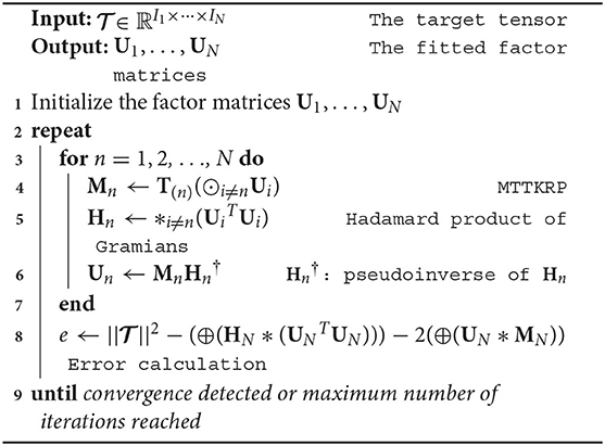
Algorithm 1. CP-ALS: Alternating least squares method for CP decomposition.

Assuming a small number of components (R), the most expensive step is the MTTKRP (line 4). This step involves 2R∏_iI_i FLOPs (ignoring, for the sake of simplicity, the lower order of FLOPs required for the computation of the KRP). The operation touches slightly more than ∏_iI_i memory locations, resulting in an arithmetic intensity less than 2R FLOPs per memory reference. Thus, unless R is sufficiently large, the speed of the computation will be limited by the memory bandwidth rather than the speed of the processor. The CP-ALS algorithm is inherently memory-bound for small R, regardless of how it is implemented.

The impact on performance of the memory-bound nature of MTTKRP is demonstrated in Figure 1, which shows the computational efficiency of a particular implementation of MTTKRP as a function of the number of components (for a tensor of size 50 × 200 × 200). Efficiency is defined as the ratio of the performance achieved by MTTKRP (in FLOPs/sec), relative to the Theoretical Peak Performance (TPP, see below) of the machine, i.e.,

$\text{EFFICIENCY}=\frac{\text{PERFORMANCE}}{\text{TPP}}=\frac{\text{\#FLOPS}/\text{TIME}}{\text{TPP}}.$

The TPP of a machine is defined as the maximum number of (double precision) floating point operations the machine can perform in 1 s. Table 1 shows the TPP for our particular machine (see Section 5 for details). In Figure 1, we see that the efficiency of MTTKRP tends to increase with the number of components, R, until eventually reaching a plateau. On this machine, the plateau is R ≥ 60 at ≈ 70% efficiency for one thread and R ≥ 300 at ≈ 35% efficiency for 24 threads. For R ≤ 20, which is common in applications, the efficiency is well below the TPP.

TABLE 1

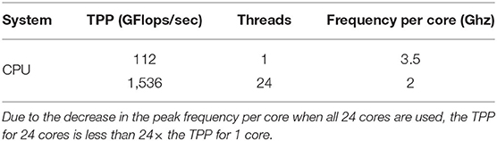
Table 1. Theoretical peak performance (TPP) for a particular machine.

FIGURE 1

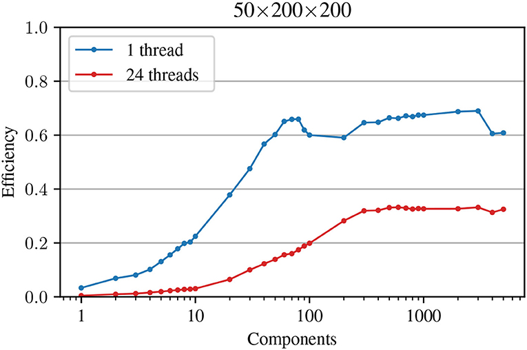
Figure 1. Efficiency of MTTKRP on a 50 × 200 × 200 tensor for an increasing number of components. Note that in the multi-threaded execution, the theoretical peak performance increases while the total number of operations to be performed stays the same (as in the single-threaded case); this explains the drop in efficiency per thread.

3.3. Concurrent ALS (CALS)

When fitting multiple CP models to the same underlying tensor, the Concurrent ALS (CALS) technique can improve the efficiency if the number of components is not large enough for CP-ALS to reach its performance plateau [7]. A need to fit multiple models to the same tensor arises, for example, when trying different initial guesses or when trying different numbers of components.

The gist of CALS can be summarized as follows (see Psarras et al. [7] for details). Suppose K independent instances of CP-ALS have to be executed on the same underlying tensor. Rather than running them sequentially or in parallel, run them in lock-step fashion as follows. Advance every CP-ALS process one iteration before proceeding to the next iteration. One CALS iteration entails K CP-ALS iterations (one iteration per model). Each CP-ALS iteration in turn contains one MTTKRP operation, so one CALS iteration also entails K MTTKRP operations. But these MTTKRPs all involve the same tensor and can therefore be fused into one bigger MTTKRP operation (see Equation 3 of Psarras et al. [7]). The performance of the fused MTTKRP depends on the sum total of components, i.e., $\sum _{i=1}^K{R}_i$, where R_i is the number of components in model i. Due to the performance profile of MTTKRP (see Figure 1), the fused MTTKRP is expected to be more efficient than each of the K smaller operations it replaces.

The following example illustrates the impact on efficiency of MTTKRP fusion. Given a target tensor of size 50 × 200 × 200, K = 50 models to fit, and R_i = 5 components in each model, the efficiency for each of the K MTTKRPs in CP-ALS is about 15% (3%) for 1 (24) threads (see Figure 1). The efficiency of the fused MTTKRP in CALS will be as observed for $R=\sum _{i=1}^K{R}_i=250$, i.e., 60% (30%) for 1 (24) threads. Since the MTTKRP operation dominates the cost, CALS is expected to be ≈ 4 × (≈ 10×) faster than CP-ALS for 1 (24) threads.

3.4. Jackknife

Algorithm 2 shows a baseline (inefficient) application of leave-one-out jackknife resampling to a CP model. For details, see Riu and Bro [4]. The inputs are a target tensor ${T}$, an overall CP model P fitted to all of ${T}$, and a sampled mode $\widehat{n}\in \left\{1,2,\dots ,N\right\}$. For each sample $p\in \left\{1,2,\dots ,I_{\widehat{n}}\right\}$, the algorihm removes the slice corresponding to the sample from tensor ${T}$ (line 3) and model P (line 4) and fits a reduced model P_−p (lines 4–6) to the reduced tensor $\widehat{{T}}$ using regular CP-ALS. After fitting all submodels, the standard deviation of every factor matrix except ${\text{U}}_{\widehat{n}}$ is computed from the $I_{\widehat{n}}$ submodels in ${Q}$ (line 10). The only costly part of Algorithm 2 is the repeated calls to CP-ALS in line 5.

ALGORITHM 2

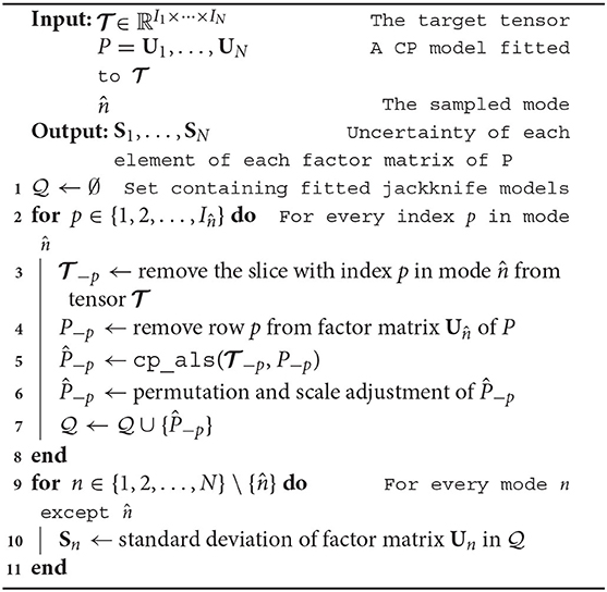
Algorithm 2. JK-ALS: An algorithm that performs (LOO) jackknife resampling on a CP model.

4. Accelerating Jackknife by Using CALS

The straightforward application of jackknife to CP in Algorithm 2 involves $I_{\widehat{n}}$ independent calls to CP-ALS on nearly the same tensor. Since the tensors are not exactly the same, CALS [7] cannot be directly applied. In this section, we show how one can rewrite Algorithm 2 in such a way that CALS can be applied. There is an associated overhead due to extra computation, but we will show that the overhead is modest (less than a 100% increase and typically only a few percent increase).

4.1. JK-CALS: Jackknife Extension of CALS

Let ${T}$ be an N-mode tensor with a corresponding CP model A₁, …, A_N. Let $\widehat{{T}}$ be identical to ${T}$ except for one sample (with index p) removed from the sampled mode $\widehat{n}\in \left\{1,2,\dots ,N\right\}$. Let ${\widehat{\text{A}}}_1,\dots ,{\widehat{\text{A}}}_N$ be the CP submodel corresponding to the resampled tensor ${T}$.

When fitting a CP model to ${T}$ using CP-ALS, the MTTKRP for mode n is given by

$\begin{array}{ll}{M}_n\leftarrow T_{(n)}(A_N\odot \cdots \odot A_n+1\odot A_n-1\odot \cdots \odot A_1).& (1)\end{array}$

Similarly, when fitting a model to $\widehat{{T}}$, the MTTKRP for mode n is given by

$\begin{array}{ll}{\widehat{\text{M}}}_n\leftarrow {\widehat{\text{T}}}_{(n)}({\widehat{\text{A}}}_N\odot \cdots \odot {\widehat{\text{A}}}_{n+1}\odot {\widehat{\text{A}}}_{n-1}\odot \cdots \odot {\widehat{\text{A}}}_1).& (2)\end{array}$

Can ${\widehat{\text{M}}}_n$ be computed from T_(n) instead of ${\widehat{\text{T}}}_{(n)}$? As we will see, the answer is yes. We separate two cases: $n=\widehat{n}$ and $n\ne \widehat{n}$.

Case I: $n=\widehat{n}$. The slice of ${T}$ removed when resampling corresponds to a row of the unfolding $\text{T}(n)=\text{T}(\widehat{n})$. To see this, note that element ${T}(i_1,i_2,\dots ,i_N)$ corresponds to element T_(n)(i_n, j) of its mode-n unfolding [28], where

$\begin{array}{ll}j=1+{\displaystyle \sum _{\begin{array}{c}k=1\\ k\ne n\end{array}}^N}(i_k-1){\displaystyle \prod _{\begin{array}{c}m=1\\ m\ne n\end{array}}^{k-1}}{I}_m.& (3)\end{array}$

When we remove sample p, then ${\widehat{\text{T}}}_{(n)}$ will be identical to T_(n) except that row p from the latter is missing in the former. In other words, ${\widehat{\text{T}}}_{(n)}={\text{E}}_p\text{T}(n)$, where E_p is the matrix that removes row p. We can therefore compute ${\widehat{\text{M}}}_n$ by replacing ${\widehat{\text{T}}}_{(n)}$ with T_(n) in Equation (2) and then discarding row p from the result:

${\widehat{\text{M}}}_n\leftarrow {\text{E}}_p({\text{T}}_{(n)}({\widehat{\text{A}}}_N\odot \cdots \odot {\widehat{\text{A}}}_{n+1}\odot {\widehat{\text{A}}}_{n-1}\odot \cdots \odot {\widehat{\text{A}}}_1)).$

Case II: $n\ne \widehat{n}$. The slice of ${T}$ removed when resampling corresponds to a set of columns in the unfolding T_(n). One could in principle remove these columns to obtain ${\widehat{\text{T}}}_{(n)}$. But instead of explicitly removing sample p from ${T}$, we can simply zero out the corresponding slice of ${T}$. To give the CP model matching dimensions, we need only insert a row of zeros at index p in factor matrix $\widehat{n}$. Crucially, the zeroing out of slice p is superfluous. In the MTTKRP, the elements that should have been zeroed out will be multiplied with zeros in the Khatri-Rao product generated by the row of zeros insert in factor matrix $\widehat{n}$. Thus, to compute ${\widehat{\text{M}}}_n$ in Equation (2) we (a) replace ${\widehat{\text{T}}}_{(n)}$ with T_(n) and (b) insert a row of zeros at index p in factor matrix ${\widehat{\text{A}}}_{\widehat{n}}$.

In summary, we have shown that it is possible to compute ${\widehat{\text{M}}}_n$ in Equation (2) without referencing the reduced tensor. There is an overhead associate with extra arithmetic. For the case $n=\widehat{n}$, we compute numbers that are later discarded. For the case $n\ne \widehat{n}$, we do some arithmetic with zeros.

4.1.1. The JK-CALS Algorithm

Based on the observations above, the CALS algorithm [7] can be modified to facilitate the concurrent fitting of all jackknife submodels. Algorithm 3 incorporates the necessary changes (colored red). The inputs are a target tensor ${T}$, and the sampled mode $\widehat{n}$. The algorithm starts by initializing $I_{\widehat{n}}$ submodels P_p for $p=1,2,\dots ,I_{\widehat{n}}$ in line 1; each submodel P_p is created by removing row p from factor matrix ${\text{U}}_{\widehat{n}}$ of model P. As described in Psarras et al. [7], CALS creates a multi-matrix n for each mode n by horizontally concatenating the factor matrices of each submodel P_p in lines 2–10; the superscript |p denotes the position in n where the factor matrix $U_n^{(p)}$ is copied. In the case of JK-CALS, instead of just copying each factor matrix into its corresponding multi-matrix, the algorithm first checks whether zero padding is required (lines 5–7). The loop in line 11 performs ALS for all submodels concurrently. Specifically, in line 13 the MTTKRP (n) is computed for all models at the same time by using the multi-matrices i. Then, lines 15 and 16 are the same as lines 5 and 6 of Algorithm 1; each submodel is treated separately by reading its corresponding values within n and n (indicated by the superscript |p). In JK-CALS, when $n=\widehat{n}$, the padded row is reset to 0 after ${\overline{U}}_n^{(|p)}$ is updated (line 18). Finally, after a full ALS cycle has completed, the error of each model is calculated in line 23. In JK-CALS, the error formula is adjusted for each submodel by considering the L2 norm of its corresponding subtensor ${{T}}_{-p}$.

ALGORITHM 3

Algorithm 3. JK-CALS: Concurrent alternating least squares method for jackknife estimation.

We remark that JK-CALS can be straightforwardly extended to grouped jackknife [10, p. 7], in which the samples are split into groups of d elements ($I_{\widehat{n}}/d$ groups) and jackknife submodels are created by removing an entire group at a time. Instead of padding and periodically zeroing out one row, we pad and periodically zero out d rows.

4.2. Performance Considerations

While Algorithm 3 benefits from improved MTTKRP efficiency, the padding results in extra arithmetic operations. Let d denote the number of removed samples (d = 1 corresponds to leave-one-out). For the sake of simplicity, assume that the integer d divides $I_{\widehat{n}}$. In grouped jackknife there are $I_{\widehat{n}}/d$ submodels, each with R components. The only costly part is the MTTKRP.

The MTTKRPs in JK-ALS (for all submodels combined) requires

$\left(\frac{I_{\widehat{n}}}{d}\right)\left(2R\left(I_{\widehat{n}}-d\right){\displaystyle \prod _{\begin{array}{c}i=1\\ i\ne \widehat{n}\end{array}}^N}{I}_i\right)$

FLOPs. Meanwhile, the fused MTTKRP in JK-CALS requires

$2\left(\frac{I_{\widehat{n}}}{d}R\right){\displaystyle \prod _{i=1}^N}{I}_i$

FLOPs. The ratio of the latter to the former comes down to

$\frac{I_{\widehat{n}}}{I_{\widehat{n}}-d}\le 2,$

since $d\le I_{\widehat{n}}/2$ in grouped jackknife. Thus, in the worst case, JK-CALS requires less than twice the FLOPs of JK-ALS. More typically, the overhead is negligible.

5. Experiments

We investigate the performance benefits of the JK-CALS algorithm to perform jackknife resampling on a CP model through two sets of experiments. In the first set of experiments, we focus on the scalability of the algorithm, with respect to both problem size and number of processor cores. For this purpose, we use synthetic datasets of increasing volume, mimicking the shape of real datasets. In the second set of experiments, we illustrate JK-CALS's practical impact by using it to perform jackknife resampling on two tensors arising in actual applications.

All experiments were conducted using a Linux-based system with an Intel® Xeon® Platinum 8160 Processor (Turbo Boost enabled, Hyper-Threading disabled), which contains 24 physical cores split in 2 NUMA regions of 12 cores each. The system also contains an Nvidia Tesla V100 GPU². The experiments were conducted with double precision arithmetic and we report results for 1 thread, 24 threads (two NUMA regions), and the GPU (with 24 CPU threads). The source code (available online³) was compiled using GCC⁴ and linked to the Intel® Math Kernel Library⁵.

5.1. Scalability Analysis

In this first experiment, we use three synthetic tensors of size 50 × m × m with m ∈ {100, 200, 400}, referred to as “small”, “medium” and “large” tensors, respectively. The samples are in the first mode. The other modes contain variables. The number of samples is kept low, since leave-one-out jackknife is usually performed on a small number of samples (usually <100), while there can be arbitrarily many variables.

For each tensor, we perform jackknife on four models with varying number of components (R ∈ {3, 5, 7, 9}). This range of component counts is typical in applications. In practice, it is often the case that multiple models are fitted to the target tensor, and many of those models are then further analyzed using jackknife. For this reason, we perform jackknife on each model individually, as well as to all models simultaneously (denoted by “All” in the figures), to better simulate multiple real-world application scenarios. In this experiment, the termination criteria based on maximum number of iterations and tolerance are ignored; instead, all models are forced to go through exactly 100 iterations, typically a small number of iterations for small values of tolerance (i.e., most models require more than 100 iterations). The reason for this choice is that we aim to isolate the performance difference of the methods tested; therefore, we maintain a consistent amount of workload throughout the experiment. (Tolerance and maximum number of iterations are instead used later on in the application experiments.)

For comparison, we perform jackknife using three methods: JK-ALS, JK-OALS and JK-CALS. JK-OALS uses OpenMP to take advantage of the inherent parallelism when fitting multiple submodels by parallelizing the loop in line 2 of Algorithm 2. Each thread maintains its own subsample ${{T}}_{-p}$ and P_−p of tensor ${T}$ and model P, respectively. This method is only used for multi-threaded and GPU experiments, and we are only going to focus on its performance, ignoring the memory overhead associated with it.

Figure 2 shows results for single threaded execution; in this case, JK-OALS is absent. JK-CALS consistently outperforms JK-ALS for all tensor sizes and workloads. Specifically, for any fixed amount of workload—i.e., a model of a specific number of components—JK-CALS exhibits increasing speedups compared to JK-ALS, as the tensor size increases. For example, for a model with 5 components, JK-CALS is 2.9, 3, 5.2 times faster than JK-ALS, for the small, medium and large tensor sizes, respectively.

FIGURE 2

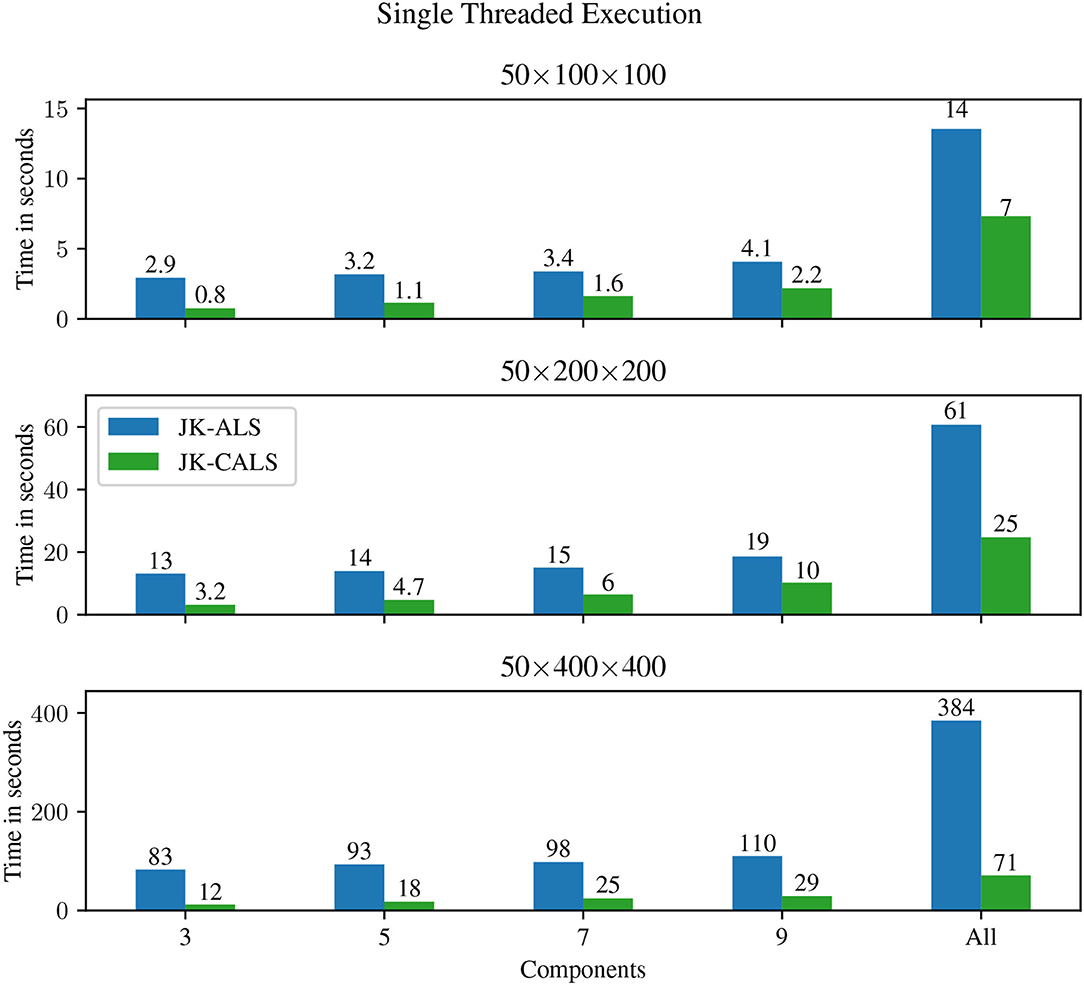
Figure 2. Execution time for single-threaded jackknife resampling applied to three different tensors (small, medium, and large in the top, middle, and bottom panels, respectively), and different number of components (from left to right: R ∈ {3, 5, 7, 9}, and “All,” which represents doing jackknife to all four models simultaneously).

Figure 3 shows results for multi-threaded execution, using 24 threads. In this case, JK-CALS outperforms the other two implementations (JK-ALS and JK-OALS) for the medium and large tensors, for all workloads (number of components), exhibiting speedups up to 35× and 8× compared to JK-ALS and JK-OALS, respectively. For the small tensor (50 × 100 × 100) and small workloads (R ≤ 7), JK-CALS is outperformed by JK-OALS; for R = 3, it is also outperformed by JK-ALS. Investigating this further, for the small tensor and R = 3 and 5, the parallel speedup (the ratio between single threaded and multi-threaded execution time) of JK-CALS is 0.3× and 0.7× for 24 threads. However, for 12 threads, the corresponding timings are 0.28 and 0.27 s, resulting in speedups of 2.7× and 3.7×, respectively. This points to two main reasons for the observed performance of JK-CALS in these cases: a) the amount of available computational resources (24 threads) is disproportionately high compared to the volume of computation to be performed and b) because of the small amount of overall computation, the small overhead associated with the CALS methodology becomes more significant.

FIGURE 3

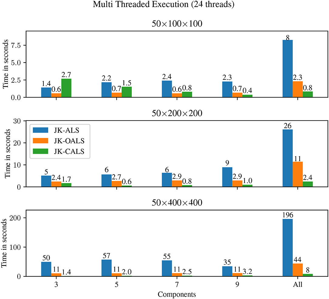
Figure 3. Execution time for multi-threaded (24 threads) jackknife resampling applied to three different tensors (small, medium, and large in the top, middle, and bottom panels, respectively), and different number of components (from left to right: R ∈ {3, 5, 7, 9}, and “All”, which represents doing jackknife to all four models simultaneously).

That being said, even for the small tensor, as the amount of workload increases—already for a single model with 9 components—JK-CALS again becomes the fastest method. Finally, similarly to the single threaded case, as the size of the tensor increases, so do the speedups achieved by JK-CALS over the other two methods.

Figure 4 shows results when the GPU is used to perform MTTKRP for all three methods; in this case, all 24 threads are used on the CPU. For the small tensor and small workloads (R ≤ 5), there is not enough computation to warrant the shipping of data to and from the GPU, resulting in higher execution times compared to multi-threaded execution; for all other cases, all methods have reduced execution time when using the GPU compared to the execution on 24 threads. Furthermore, in those cases, JK-CALS is consistently faster than its counterparts, exhibiting the largest speedups when the workload is at its highest (“All”), with values of 10×, 7×, 7× compared to JK-OALS, and 12×, 10×, 9× compared to JK-ALS, for the small, medium and large tensors, respectively.

FIGURE 4

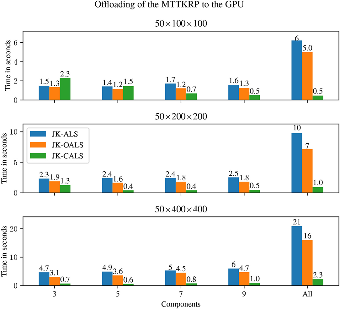
Figure 4. Execution time for GPU + multi-threaded (GPU + 24 threads) jackknife resampling applied to three different tensors (small, medium, and large in the top, middle, and bottom panels, respectively), and different number of components (from left to right: R ∈ {3, 5, 7, 9}, and “All”, which represents doing jackknife to all four models simultaneously).

5.2. Real-World Applications

In this second experiment, we selected two tensors of size 89 × 97 × 549 and 44 × 2700 × 200 from the field of Chemometrics [30, 31]. In this field it is common to fit multiple, randomly initialized models in a range of low components (e.g., R ∈ {1, 2, …, 20}, 10–20 models for each R, and then analyze (e.g., using jackknife) those models that might be of particular interest (often those with components close to the expected rank of the target tensor); in the tensors we consider, the expected rank is 5 and 20, respectively. To mimic the typical workflow of practitioners, we fitted three models to each tensor, of components R ∈ {4, 5, 6} and R ∈ {19, 20, 21}, respectively, and used the three methods (JK-ALS, JK-OALS and JK-CALS) to apply jackknife resampling to the fitted models⁶. The values for tolerance and maximum number of iterations were set according to typical values for the particular field, namely 10⁻⁶ and 1, 000, respectively.

In Figure 5 we report the execution time for 1 thread, 24 threads, and GPU + 24 threads. For both datasets and for all configurations, JK-CALS is faster than the other two methods. Specifically, when compared to JK-ALS over the two tensors, JK-CALS achieves speedups of 5.4× and 2× for single threaded execution, 10× and 2.8× for 24-threaded execution. Similarly, when compared to JK-OALS, JK-CALS achieves speedups of 2.7× and 4.8× for 24-threaded execution. Finally, JK-CALS takes advantage of the GPU the most, exhibiting speedups of 17.5× and 3.7× over JK-ALS, and 9× and 2× over JK-OALS, for GPU execution.

FIGURE 5

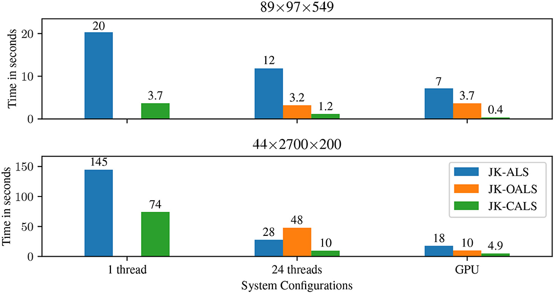
Figure 5. Execution time for jackknife resampling applied to two applications tensors. For tensor 89 × 97 × 549, whose expected rank is 5, three models with R ∈ {4, 5, 6} were fitted and then jackknife was applied to them (i.e., the “All” group from the previous section). Similarly, for tensor 44 × 2, 700 × 200, whose expected rank is 20, three models with R ∈ {19, 20, 21} were fitted and then jackknifed. In both cases, tolerance and maximum number of iterations were set to 10⁻⁶ and 1, 000, respectively.

6. Conclusion

Jackknife resampling of CP models is useful for estimating uncertainties, but the computation requires fitting multiple submodels and is therefore computationally expensive. We presented a new technique for implementing jackknife that better utilizes the computer's memory hierarchy. The technique is based on a novel extension of the Concurrent ALS (CALS) algorithm for fitting multiple CP models to the same underlying tensor, first introduced in Psarras et al. [7]. The new technique has a modest arithmetic overhead that is bounded above by factor of two in the worst case. Numerical experiments on both synthetic and real-world datasets using a multicore processor paired with a GPU demonstrated that the proposed algorithm can be several times faster than a straightforward implementation of jackknife resampling based on multiple calls to a regular CP-ALS implementation.

Future work includes extending the software to support grouped jackknife.

Data Availability Statement

Publicly available datasets were analyzed in this study. This data can be found here: https://github.com/HPAC/CP-CALS/tree/jackknife.

Author Contributions

CP drafted the main manuscript text, developed the source code, performed the experiments, and prepared all figures. LK and PB revised the main manuscript text. CP, LK, and PB discussed and formulated the jackknife extension of CALS. CP, LK, RB, and PB discussed and formulated the experiments. LK, RB, and CP discussed the related work section. PB oversaw the entire process. All authors reviewed and approved the final version of the manuscript.

Funding

This work was funded by the Deutsche Forschungsgemeinschaft (DFG, German Research Foundation)–333849990/GRK2379 (IRTG Modern Inverse Problems).

Conflict of Interest

The authors declare that the research was conducted in the absence of any commercial or financial relationships that could be construed as a potential conflict of interest.

Publisher's Note

All claims expressed in this article are solely those of the authors and do not necessarily represent those of their affiliated organizations, or those of the publisher, the editors and the reviewers. Any product that may be evaluated in this article, or claim that may be made by its manufacturer, is not guaranteed or endorsed by the publisher.

Footnotes

1. ^Henceforth, when we mention jackknifing we imply LOO jackknifing, unless otherwise stated.

2. ^Driver version: 470.57.02, CUDA Version: 11.2.

3. ^https://github.com/HPAC/CP-CALS/tree/jackknife

4. ^GCC version 9.

5. ^MKL version 19.0.

6. ^The same models were given as input to the three methods, and thus require the same number of iterations to converge.

References

1. Murphy KR, Stedmon CA, Graeber D, Bro R. Fluorescence spectroscopy and multi-way techniques. PARAFAC. Anal Methods. (2013) 5:6557–66. doi: 10.1039/c3ay41160e

CrossRef Full Text | Google Scholar

2. Wiberg K, Jacobsson SP. Parallel factor analysis of HPLC-DAD data for binary mixtures of lidocaine and prilocaine with different levels of chromatographic separation. Anal Chim Acta. (2004) 514:203–9. doi: 10.1016/j.aca.2004.03.062

CrossRef Full Text | Google Scholar

3. Farrance I, Frenkel R. Uncertainty of measurement: a review of the rules for calculating uncertainty components through functional relationships. Clin Biochem Rev. (2012) 33:49–75.

PubMed Abstract | Google Scholar

4. Riu J, Bro R. Jack-knife technique for outlier detection and estimation of standard errors in PARAFAC models. Chemom Intell Lab Syst. (2003) 65:35–49. doi: 10.1016/S0169-7439(02)00090-4

CrossRef Full Text | Google Scholar

5. Kiers HAL. Bootstrap confidence intervals for three-way methods. J Chemom. (2004) 18:22–36. doi: 10.1002/cem.841

CrossRef Full Text | Google Scholar

6. Martens H, Martens M. Modified Jack-knife estimation of parameter uncertainty in bilinear modelling by partial least squares regression (PLSR). Food Qual Prefer. (2000) 11:5–16. doi: 10.1016/S0950-3293(99)00039-7

CrossRef Full Text | Google Scholar

7. Psarras C, Karlsson L, Bientinesi P. Concurrent alternating least squares for multiple simultaneous canonical polyadic decompositions. arXiv preprint arXiv:2010.04678. (2020).

8. Westad F, Marini F. Validation of chemometric models – a tutorial. Anal Chim Acta. (2015) 893:14–24. doi: 10.1016/j.aca.2015.06.056

PubMed Abstract | CrossRef Full Text | Google Scholar

9. Peddada SD. 21 Jackknife variance estimation and bias reduction. In: Computational Statistics. Vol. 9 of Handbook of Statistics. Elsevier (1993). p. 723–44. Available online at: https://www.sciencedirect.com/science/article/pii/S0169716105801452.

10. Efron B. The jackknife, the bootstrap and other resampling plans. In: Society for Industrial and Applied Mathematics. (1982). Available online at: https://epubs.siam.org/doi/book/10.1137/1.9781611970319

PubMed Abstract | Google Scholar

11. Kott PS. The delete-a-group jackknife. J Off Stat. (2001) 17:521. Available online at: https://www.scb.se/dokumentation/statistiska-metoder/JOS-archive/

12. Sanchez E, Kowalski BR. Generalized rank annihilation factor analysis. Anal Chem. (1986) 58:496–9. doi: 10.1021/ac00293a054

CrossRef Full Text | Google Scholar

13. Acar E, Dunlavy DM, Kolda TG. A scalable optimization approach for fitting canonical tensor decompositions. J Chemom. (2011) 25:67–86. doi: 10.1002/cem.1335

CrossRef Full Text | Google Scholar

14. Rajih M, Comon P, Harshman RA. Enhanced line search: a novel method to accelerate PARAFAC. SIAM J Matrix Anal Appl. (2008) 30:1128–47. doi: 10.1137/06065577

CrossRef Full Text | Google Scholar

15. Shun Ang AM, Cohen JE, Khanh Hien LT, Gillis N. Extrapolated alternating algorithms for approximate canonical polyadic decomposition. In: ICASSP 2020-2020 IEEE International Conference on Acoustics, Speech and Signal Processing (ICASSP). Barcelona: IEEE (2020). p. 3147–51.

16. Vervliet N, De Lathauwer L. A randomized block sampling approach to canonical polyadic decomposition of large-scale tensors. IEEE J Sel Top Signal Process. (2016) 10:284–95. doi: 10.1109/JSTSP.2015.2503260

CrossRef Full Text | Google Scholar

17. Battaglino C, Ballard G, Kolda TG. A practical randomized CP tensor decomposition. SIAM J Matrix Anal Appl. (2018) 39:876–901. doi: 10.1137/17M1112303

CrossRef Full Text | Google Scholar

18. Bro R, Andersson CA. Improving the speed of multiway algorithms: part II: compression. Chemom Intell Lab Syst. (1998) 42:105–13. doi: 10.1016/S0169-7439(98)00011-2

CrossRef Full Text | Google Scholar

19. Solomonik E, Matthews D, Hammond J, Demmel J. Cyclops tensor framework: reducing communication and eliminating load imbalance in massively parallel contractions. In: 2013 IEEE 27th International Symposium on Parallel and Distributed Processing. Cambridge, MA: IEEE (2013). p. 813–24.

20. Kannan R, Ballard G, Park H. A high-performance parallel algorithm for nonnegative matrix factorization. SIGPLAN Not. (2016) 51:1–11. doi: 10.1145/3016078.2851152

CrossRef Full Text | Google Scholar

21. Lourakis G, Liavas AP. Nesterov-based alternating optimization for nonnegative tensor completion: algorithm and parallel implementation. In: 2018 IEEE 19th International Workshop on Signal Processing Advances in Wireless Communications (SPAWC). Kalamata: IEEE (2018). p. 1–5.

22. Smith S, Ravindran N, Sidiropoulos ND, Karypis G. SPLATT: efficient and parallel sparse tensor-matrix multiplication. In: 2015 IEEE International Parallel and Distributed Processing Symposium. Hyderabad: IEEE (2015). p. 61–70.

23. Phipps ET, Kolda TG. Software for sparse tensor decomposition on emerging computing architectures. SIAM J Sci Comput. (2019) 41:C269–90. doi: 10.1137/18M1210691

CrossRef Full Text | Google Scholar

24. Psarras C, Karlsson L, Li J, Bientinesi P. The landscape of software for tensor computations. arXiv preprint arXiv:2103.13756. (2021).

25. Buzas JS. Fast estimators of the jackknife. Am Stat. (1997) 51:235–40. doi: 10.1080/00031305.1997.10473969

PubMed Abstract | CrossRef Full Text | Google Scholar

26. Belotti F, Peracchi F. Fast leave-one-out methods for inference, model selection, and diagnostic checking. Stata J. (2020) 20:785–804. doi: 10.1177/1536867X20976312

CrossRef Full Text | Google Scholar

27. Hinkle JE, Stromberg AJ. Efficient computation of statistical procedures based on all subsets of a specified size. Commun Stat Theory Methods. (1996) 25:489–500. doi: 10.1080/03610929608831709

CrossRef Full Text | Google Scholar

28. Kolda TG, Bader BW. Tensor decompositions and applications. SIAM Rev. (2009) 51:455–500. doi: 10.1137/07070111X

CrossRef Full Text | Google Scholar

29. Phan AH, Tichavský P, Cichocki A. Fast alternating LS algorithms for high order CANDECOMP/PARAFAC tensor factorizations. IEEE Trans Signal Process. (2013) 61:4834–4846. doi: 10.1109/TSP.2013.2269903

CrossRef Full Text | Google Scholar

30. Acar E, Bro R, Schmidt B. New exploratory clustering tool. J Chemom. (2008) 22:91–100. doi: 10.1002/cem.1106

CrossRef Full Text | Google Scholar

31. Skov T, Ballabio D, Bro R. Multiblock variance partitioning: a new approach for comparing variation in multiple data blocks. Anal Chim Acta. (2008) 615:18–29. doi: 10.1016/j.aca.2008.03.045

PubMed Abstract | CrossRef Full Text | Google Scholar