A kernel mixing strategy for use in adaptive Markov chain Monte Carlo and stochastic optimization contexts

1. Introduction

Mathematical models can be used to study the behavior of many physical systems in the world. In most cases, however, these models contain many unknown parameters which must be tuned in order for the model to accurately replicate the behavior of the system of interest. This problem of fitting the parameters of a mathematical model to data—as well as the related problem of uncertainty quantification of said model parameters—is a staple problem in applied mathematics. We can represent it as an optimization problem. Suppose we are given model f(θ) (with parameters θ) and data y. We must solve the problem

$\begin{array}{ll}{\displaystyle \underset{\theta }{min}}\left|\right|f(\theta )-y\left|\right|,& (1)\end{array}$

where ||·|| is some chosen norm. The value of θ which minimizes this error can be found via various global optimization methods and with subsequent analysis of uncertainty via sampling methods. However, the efficiency of these methods depends largely on various hyper-parameters (parameters that define the behavior of the optimizer) which must be set. For this reason, methods with robust adaptive features which are able to tune themselves to the problem at hand are preferred.

In this paper, we will present a new local kernel mixing method which can be implemented in various global optimization methods and sampling methods. This method mixes several Gaussian kernels with varying covariance matrices so that an overall underestimation or overestimation of the covariance matrix for the particular applied problem will have less significant of an impact on performance. We specifically test this mixing method's performance in a simulated annealing (SA), real-coded genetic algorithm (GA), and Markov chain Monte Carlo (MCMC) context. All three of these methods have a similar underlying scheme for generating new solutions from Gaussian perturbations and are thus prime candidates for testing our method.

We will begin with a brief overview of the MCMC, SA, and GA algorithms. We will then discuss the kernel mixing method, its properties, and how it can be implemented. We then test the three algorithms performance with and without our kernel mixing scheme on two popular benchmark problems: the Ackley function and the thermal isomerization of α-pinene.

1.1. The Metropolis method

The Metropolis method—the original Markov Chain Monte Carlo (MCMC) approach developed by Metropolis et al. [1] and later generalized by Hastings [3]—is the foundation for all subsequent MCMC approaches. Given some data y (often given in the form of a time series or vector) and a model which can reproduce them, the Metropolis method samples the posterior distribution π(θ|y) of the model's parameters. This distribution describes the probability of the model parameters' values given the data. This distribution will have a peak at the values of the model parameters which best approximate the data.

However, as its name would imply, we do not have a priori knowledge of the posterior distribution. Therefore, we express the posterior distribution in terms of distributions we know using Bayes's Theorem

$\begin{array}{ll}\pi (\theta |y)\propto \ell (y|\theta )p(\theta ),& (2)\end{array}$

where ℓ is the likelihood distribution and p is the prior distribution. The likelihood ℓ(y|θ) tells us the probability of the data given the parameters and is usually calculated from the model-data error

$\begin{array}{ll}\ell (y|\theta )\propto \text{exp}(-||f(\theta )-y|{|}^2/(2{\sigma }^2)),& (3)\end{array}$

where ||·|| is the appropriate norm and σ is the measurement error. This can be easily calculated via a single model evaluation with the given parameters. We may also have additional information about what parameter values are most likely to be realized in the actual system. For example, perhaps the parameters are uniformly distributed over a bounded space. This information is incorporated via the prior distribution p. Together, the likelihood and prior help us to reconstruct the posterior distribution up to a scale factor.

Let us look at how Metropolis performs its sampling. Given an initial state θ⁰ (superscript indices will refer to the time step), Metropolis generates new candidate states and probabilistically accepts or rejects them based on relative posterior gains or losses with respect to that of current state. Candidate state generation is performed via sampling of the proposal distribution q(θ′|θⁿ), defined as the probability that a new state θ′ will be selected as a candidate for acceptance given the current state θⁿ. The most common choice of proposal distribution is the standard multivariate Gaussian distribution. Whether acceptance or rejection is performed is determined by the acceptance probability α(θ′|θⁿ), defined as the probability that the candidate state θ′ will be accepted given the current step θⁿ (see Algorithm 1 for the calculation of the acceptance probability). The unification of these candidate generation and acceptance steps is the kernel of the method, which defines the transition probabilities between states. Over time, the distribution created from the samples will conform to the posterior, at which point the method is said to have converged. Algorithm 1 shows a pseudocode implementation of Metropolis.

ALGORITHM 1

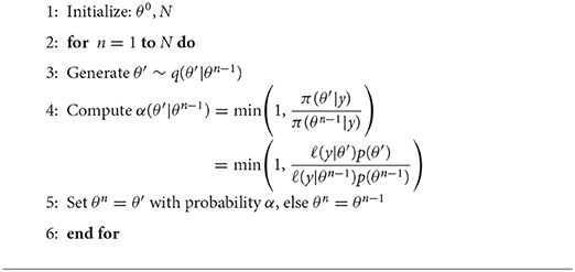
Algorithm 1. The Metropolis method

Metropolis is ergodic and is therefore guaranteed to converge to the correct stationary distribution if given sufficient time. However, the time to converge depends largely on the proposal distribution used. As stated, the preferred proposal distribution is Gaussian, whose width is defined by a covariance matrix (in fact, the term proposal width is often used in its place). If one chooses too thin of a Gaussian, the chain may have difficulty escaping suboptimal modes within a reasonable amount of time. On the other hand, too wide and the chain will have an excess of rejections. Fortunately, this problem of the unknown proposal can be largely alleviated through clever means such as kernel mixing and adaptive proposals.

Kernel mixing (or more precisely proposal mixing, since kernel would refer to the composition of the proposal and acceptance steps) is a technique where the proposal used at each step in the chain may be chosen stochastically from a set. Consider an example where we have two proposals Q₁, Q₂ and we have a probability 0.5 of choosing either at any given step. Then, the proposal used at each step is simply 0.5Q₁+0.5Q₂—the linear combination of the kernels and their respective probabilities. This is implemented by choosing either Q₁ or Q₂ at each step.

Another technique for improving the performance of MCMC is to use so-called adaptive methods which allow the proposal to adapt to the state space as more and more samples are obtained. Likely the most widely used adaptive MCMC method is Haario's Adaptive Metropolis (AM) [2] method. The core principle of adaptation is the use of a continuously adapting Gaussian distribution as the proposal for the standard Metropolis method. After beginning with an initial phase of non-adaptation called the burn-in, the proposal becomes

$\begin{array}{ll}{q}^n({\theta }^{\prime }|{\theta }^n)=N\left({\theta }^n,\left(\frac{{2.38}^2}{M}\right){\Sigma }^n+\epsilon I\right),& (4)\end{array}$

where M is the dimension of the space (i.e., number of parameters), Σⁿ is the covariance matrix computed from samples generated over past steps, and ε is a small factor multiplied by an M × M identity matrix included for regularization to ensure positive-definiteness. This allows the Gaussian to continually re-scale and re-orient itself as it “learns” the state space.

The AM proposal can also be modified via kernel mixing. A good example of this is the version developed by Roberts and Rosenthal [4]

$\begin{array}{ll}{q}^n({\theta }^{\prime }|{\theta }^n)=\beta N({\theta }^n,\left(\frac{{2.38}^2}{M}\right){\Sigma }^n)+(1-\beta )N({\theta }^n,\widehat{\Sigma }),& (5)\end{array}$

where $\widehat{\Sigma }$ is a fixed covariance matrix and 0 ≤ β ≤ 1 [note that our convention is different from theirs in that we have swapped the β and (1−β) terms].

1.2. Simulated annealing

Simulated annealing [5] is a global optimization method with many similar properties to the Metropolis method. Both use proposal distributions to generate candidate solutions followed by an acceptance criterion. The main difference is the cooling aspect of SA which causes it to be more restrictive and therefore less likely to accept candidates worse than the current state. Instead of the likelihood function, SA converts the model-data error into a fitness value which is then maximized (instead of minimizing the error). This is given by

$\begin{array}{ll}F(\theta )=\text{exp}(-||f(\theta )-y||/T^n),& (6)\end{array}$

where Tⁿ is the temperature which is cooled over time. Various cooling schedules may be used, such as exponentially or logarithmically decreasing schedules and schedules which periodically raise and lower the temperature [6, 7]. For this paper we use an exponential cooling schedule

$\begin{array}{ll}{T}^n=T^0\text{exp}(-n/\tau ),& (7)\end{array}$

where τ is the cooling factor. SA can be described by Algorithm 2. Note the directing analogy between this and Algorithm 1.

ALGORITHM 2

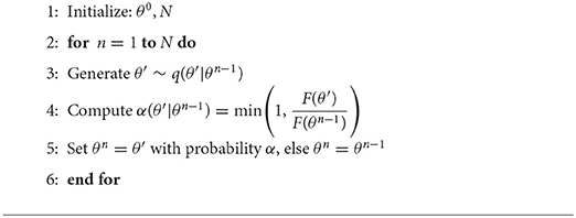
Algorithm 2. Simulated annealing

1.3. Real-coded genetic algorithms (GA)

For some complex optimization problems, simpler methods such as gradient descent and even simulated annealing are not robust enough to find the global optimum. In these cases, a popular alternative is the genetic algorithm (GA) (see the early paper by Holland [8]). Taking inspiration from biological processes, GAs solve problems by tackling them with an entire population of solutions which evolve and improve over time in a survival-of-the-fittest fashion. Though the original GA proposed by Holland used a binary encoding, many other researchers have used real-coded or real-valued GAs (see [9–11]). We will be using the real-coded scheme. Algorithm 3 shows the architecture of a canonical GA, which is very modular by nature. In the Algorithm, we define P^{j, i} as the i-th solution in the j-th generation. Let us look more closely at each of these steps.

ALGORITHM 3

Algorithm 3. Real-coded genetic algorithm for image similarity optimization

The GA's representation is simply how solutions to the problem are encoded in the individuals in the population. In the case of real-coded GAs, the representation is simply a vector of the model parameters.

Selection is the process by which individuals are paired off as parents for mating. The most popular techniques for accomplishing this are roulette selection [8] (where an individual's selection probability is proportional to its fitness) and rank selection [12] (where an individual's selection probability is proportional to its rank). Each of these operators has its own pros and cons. In roulette selection, solutions with significantly higher fitness have a proportionately higher selection probability. This can help speed up convergence. However, anomalously high fit individuals can saturate the population with their genetic material, while anomalously low fit individuals will rarely be selected. Both of these phenomena result in a decrease in genetic diversity, likely leading to premature convergence to local optima. Rank selection solves this problem by making the selection probabilities very stable (with fixed upper and lower bounds on the probabilities throughout an entire run). The question of which selection operator is optimal is highly problem-dependent and there is no clear answer. We used roulette selection in all of our GA tests.

An additional feature which may be included in the selection step is elitism [13]. This feature ensures that the best solutions are retained to the next generation by explicitly preserving them across generations. We also use elitism for our GA tests.

Next, the GA's crossover operator breeds child solutions from the selected parent pairs. This operator creates these children by combining the genetic material of the parents. Depending on preference, one can create a single child from each parent pair or two which replace both parents in the population (in second case, half as many parent pairs are selected). For the case of real-coded GAs, all of the binary coded crossover operators are available (such as single-point, multi-point, and uniform crossover) with additional options due to the nature of the encoding. A common one is arithmetic crossover [14]

$\begin{array}{ll}{C}^1=\alpha P^1+(1-\alpha )P^2,& (8)\end{array}$

$\begin{array}{ll}{C}^2=(1-\alpha )P^1+\alpha P^2,& (9)\end{array}$

where P¹, P² are the two parent solutions, C¹, C² are the two child solutions, and α∈[0, 1] is uniformly distributed. Many different versions of this scheme exist with various types of weighted means and distributions from which α may be drawn. For our purposes, we use a version of arithmetic crossover with the parents weighted by their fitnesses:

$\begin{array}{ll}C=\widehat{F}(P^1)P^1+\widehat{F}(P^2)P^2.& (10)\end{array}$

Here, $\widehat{F}(P^1)=F(P^1)/(F(P^1)+F(P^2))$ and $\widehat{F}(P^2)=F(P^2)/(F(P^1)+F(P^2))$.

Finally, the mutation operator is performed on the resulting child solutions. This operators applies a stochastic perturbation to the child chromosomes in order to preserve a sufficient level of genetic diversity in the population throughout the evolution of the population. This perturbation is done via a chosen kernel distribution. Various choices are available for this kernel. Examples include Eshelmen et al.'s blend crossover operator (BLX-α) [15] and Ono and Kobayashi's unimodal normal distribution crossover operator (UNDX) [16]. One popular technique is to introduce a degree of determinism by directing mutation along the some particular direction determined by, say, the gradient of the objective function or the momentum of the population in parameter space [17–19]. We use an adaptive mixture of multiple multivariate normal distributions with varying covariance matrices as our chosen kernel.

2. Kernel mixing method

We now discuss our kernel mixing method. We will begin with a discussion of the motivation and advantages our using this method. We then discuss the mathematics and implementation of the method in case of both diagonal and non-diagonal covariance matrices.

2.1. Motivation and advantages

Incorporation of our kernel mixing method into either stochastic optimization or MCMC contexts results in several advantages. First, as we have discussed, it isn't possible in general to know a priori what the optimal proposal width should be for a given problem. This makes adaptive methods attractive. However, even if one were to choose the optimal “global” proposal width, this by no means guarantees that certain regions of parameter space might not have a superior “local” optimal proposal width. By applying our kernel mixing method, the proposal can cover a range of widths for different parameters.

A second advantage is that when used in an MCMC context, no initial greedy search is required find a good starting point in parameter space. This is because our mixing method provides an increase in performance in optimization contexts. This performance gain is inherited by MCMC implementations of the method.

Additional advantages that our method has over some more complex methods are its trivial implementation and the minimal overhead it requires. The only significant computational overhead encountered is the diagonalization of non-diagonal covariance matrices. This overhead is only relevant when there is a very large number of parameters and the covariance matrices is adaptive, requiring constant diagonalization.

2.2. The method

Our mixing strategy allows for the selection of one of three proposals: (1) the original, fixed proposal, (2) a thinned proposal, and (3) a widened proposal. We included both the thinner and wider proposals since overestimation and underestimation the proposal width are both possible. Additionally, the thin proposal allows the chain to squeeze into thinner modes while the wide proposal allows the chain to escape suboptimal modes and traverse parameter space quickly. The resulting proposal for a simple problem with one parameter has the form of the linear combination

$\begin{array}{ll}q\left({\theta }^{\prime }|{\theta }^n\right)=p_{t}N\left({\theta }^n,{\left(A_t\sigma \right)}^2\right)+p_{f}N\left({\theta }^n,{\left(\sigma \right)}^2\right)+p_{w}N\left({\theta }^n,{\left(A_w\sigma \right)}^2\right),& (11)\end{array}$

where σ is the fixed proposal width, 0 < A_t <1 < A_w are the mixing amplitudes, and p_t, p_f, p_w are the mixing probabilities. This resulting mixture of Gaussians (each with a different variance) will not necessarily have the same variance as the original fixed variance σ². However, given the thinning and widening amplitudes A_t, A_w, the mixing probabilities can be set so that the mixed proposal will have identical variance as the fixed proposal. This is useful if one desires to have control over the variance of the mixed proposal. The probabilities that accomplish this are given by

$\begin{array}{ll}(p_t,p_f,p_w)=\left(\frac{(A_w^2-1)(1-p_f)}{(A_w^2-A_t^2)},p_f,\frac{(1-A_t^2)(1-p_f)}{(A_w^2-A_t^2)}\right),& (12)\end{array}$

where the fixed probability p_f is a free parameter, i.e., any value 0 ≤ p_f ≤ 1 will result in the same fixed variance.

Figure 1 illustrates a standard 2D Gaussian distribution and a mixture of Gaussians according to the method described above. We have mixing probabilities of (1/3, 1/3, 1/3) and mixing amplitudes of (1/3, 1, 3). There are two main features to notice in the mixed plot. First, is the overall cross shape of the distribution, with a high probability density along and near the parameter axes. Second is that the peak density in the center is higher in the mixed kernel than the standard Gaussian.

FIGURE 1

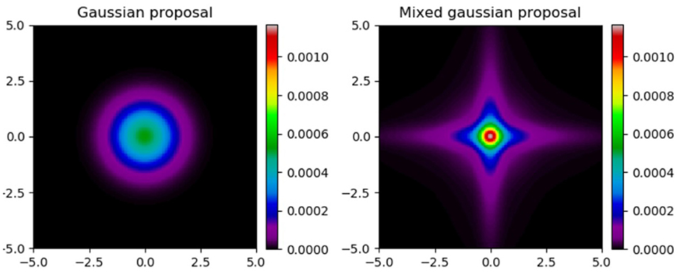
Figure 1. (Left) Standard Gaussian proposal. (Right) Mixed proposal.

In the case of M parameters, each one is mixed independently (i.e., one parameter could be thinned while another is widened). Therefore, one must account for all combinations of each parameter being mixing in each of the three ways:

$\begin{array}{l}q({\theta }^{\prime }|{\theta }^n)={\displaystyle \sum _{i_1\in \{t,f,w\}}\cdots }{\displaystyle \sum _{i_M\in \{t,f,w\}}{p}_{i_1}}\cdots p_{i_M}N{({\theta }^n,(A_{i_1}{\sigma }_1)}^2,\\ \cdots ,{(A_{i_M}{\sigma }_M)}^2).& (13)\end{array}$

For convenience in the above, we define A_f = 1 and $N(\mu ,{\sigma }_1^2,\cdots ,{\sigma }_M^2)$ as an M-dimensional normal distribution with diagonal covariance matrix given by $({\sigma }_1^2,\cdots ,{\sigma }_M^2)$.

2.3. Implementation

Regarding implementation, mixing for diagonal covariance matrices is applied according to Algorithm 4. Given a fixed diagonal covariance matrix Σ, a new covariance matrix Σ′ (initially the identity matrix I) is constructed by multiplying the diagonal elements of Σ by the square of the chosen mixing amplitude. Note that this is equivalent to multiplying the eigenvalues by the amplitudes.

ALGORITHM 4

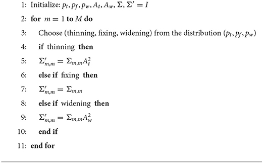
Algorithm 4. Mixing implementation for diagonal covariance matrices

For general, non-diagonal covariance matrices, Algorithm 5 is used. The significant differences are the diagonalization steps (2, 13) to obtain the eigenvalues. In the diagonal case, these were already given, but in the non-diagonal case, they must be calculated. The ability to apply this mixing procedure to non-diagonal matrices implies that it may be used in optimization and MCMC algorithms with adaptive covariance matrices, such as Haario's Adaptive Metropolis algorithm [2]. This merely requires the diagonalization of the covariance matrix at each step in the algorithm.

ALGORITHM 5

Algorithm 5. Mixing implementation for non-diagonal covariance matrices

We developed a Python implementation of our method which can be accessed at https://github.com/gtw2i/Adaptive-Kernel-Mixing-for-MCMC-and-SO. It includes all codes which were used to obtain the results in the following section, as well as the α-pinene reaction data.

3. Numerical experiments and results

We now present tests of our mixing technique in SA, GA, and MCMC contexts. In the SA case, we compare both standard SA and mixed SA with modified versions using an adaptive proposal (following the pattern of AM). Solonen [20] illustrates the difficulties in weighting the samples when applying the AM technique in the SA context (the changing temperature affects a change in the posterior). They propose multiple possible solutions to this challenge. Since our goal was to propose a mixing method rather than an adaptive method, we take a very simplistic approach to adaptation. Like AM, we accumulate samples over a burn-in period, after which their covariance matrix is calculated. However, we do not continue to adapt the matrix any further. We leave it to others to decide what the proper adaptive method for their application should be. In the GA case, we compare a real-coded GA with a Gaussian mutation operator to one which uses our mixing technique, as well as their adaptive counterparts. Like the SA implementation of proposal adaptation, we accumulate samples (the entire population at each generation) until the burn-in time is reached, at which point the covariance matrix is evaluated and subsequently held fixed. In the MCMC case, we compare Metropolis and Adaptive Metropolis with versions which use our mixing technique. Tests on all three methods are done via two benchmark problems, which will be discussed below.

We perform one test in the SA and GA cases and two in the MCMC case, each of which uses an ensemble of runs over a range of proposal widths. This will allow us to check for both best-case and average performance for each method. The test for the SA and GA cases is a simple averaging of the best fitness at each time step over an ensemble of runs. By “best” fitness, we mean to say we keep track of the highest fitness achieved by the method at each step, rendering the sequence of fitnesses non-decreasing. This allows us to examine the average rate at which the fitness improves across a broad range of proposal widths. What we will see is that each method has an optimal range of proposal widths at which fitness increases most quickly. Deviations from this optimal region slow performance. The mixing and adaptation techniques implemented serve to extend this range so that performance is less sensitive to one's choice of proposal width.

The first MCMC test calculates a lower bound of the integrated auto-correlation time (IAC) for the chain. The IAC is a measure of the length of time (in steps) required for later steps in the chain to become de-correlated with earlier steps. It is given by the formula

$\begin{array}{ll}{\tau }_{int}=1+2{\displaystyle \sum _{\ell =0}^{N^{\prime }}}{r}_{\ell },& (14)\end{array}$

where r_ℓ is the autocorrelation of the chain at lag ℓ (an index offset) and N′ is some number of steps in the chain (usually the step at which r_ℓ reaches zero). This only measures a lower bound since—in many cases—N′ is prohibitively large. For this reason, we simply choose the value of the IAC at some preset value of N′ (usually N_step/8). By generating an ensemble of chains, we obtain statistics on this lower bound for the IAC across a range of proposal widths.

The second test uses the scale reduction factor (SRF) [21]. This tests utilizes an ensemble of chains initialized at random locations and compares the values of the between-chain variance B and the within-chain variance W. Given M chains of length N, the SRF is given by $R=\sqrt{\widehat{V}/W}$ where

$\begin{array}{ll}B=\frac{N}{M-1}{\displaystyle \sum _{m=1}^M}{({\widehat{\theta }}_m-\widehat{\theta })}^{2}W=\frac{1}{M}{\displaystyle \sum _{m=1}^M}{\widehat{\sigma }}_m,& (15)\end{array}$

$\begin{array}{ll}\widehat{V}=\frac{N-1}{N}W+\frac{M+1}{MN}B,& (16)\end{array}$

where ${\widehat{\theta }}_m,{\widehat{\sigma }}_m$ are the sample mean and variance of the m-th chain and $\widehat{\theta }$ is the overall sample mean across all m chains. Since the test itself requires an ensemble of chains, we do not obtain statistics for the SRF. However, we do still calculate it over a range of proposal widths.

3.1. Benchmark 1: Ackley function

For our first benchmark, we use the Ackley function, given by

$\begin{array}{l}f(\theta )=a\left(1-\text{exp}(-0.2\sqrt{{\displaystyle \sum _{m=1}^M{\theta }_m^2}/M})\right)\\ +b\left(e-\text{exp}({\displaystyle \sum _{m=1}^M\text{cos}}(2\pi {\theta }_m)/M)\right),& (17)\end{array}$

where a = 20, b = 4, and M = 5 is the number of dimensions. This is a common benchmark function in optimization contexts since it has a large number of false minima in which chains may become stuck. For the SA and GA cases, we calculate fitness F via

$\begin{array}{ll}F(\theta )=\frac{1}{1+f{(\theta )}^2}.& (18)\end{array}$

For the MCMC case, we used a uniform prior distribution over the entire search space and used the likelihood function

$\begin{array}{ll}\ell (y|\theta )=\text{exp}(-\frac{f{(\theta )}^2}{2{\sigma }^2}),& (19)\end{array}$

where σ = 5 (this value was chosen since it resulted in an acceptance rate of between 0.25 and 0.5).

3.1.1. Simulated annealing

Now, we present the results of the SA test on the 5D Ackley function (see Figure 2). We have standard SA, mixed SA, adaptive SA, and mixed/adaptive SA. The parameter space is set to θ_m∈[−10, 10] for m = 1, ⋯ , 5. In each case, we ran 50 randomly initialized instances of the particular SA implementation over 40 evenly-spaced proposal widths. The mixing amplitudes used were (A_t, A_w) = (1/3, 3) and the mixing probabilities used were (p_t, p_f, p_w) = (3/5, 1/3, 1/15). The choice of amplitudes spans roughly an order of magnitude while the probabilities were derived by setting p_f = 1/3 and deriving the other two from Equation (12). Also, both the cooling constant τ and the burn-in time were set to be half the total number of time steps.

FIGURE 2

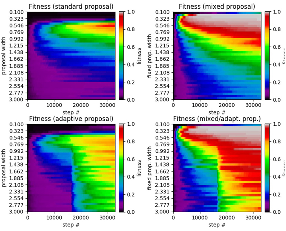
Figure 2. Results of SA test on the 5D Ackley function. (Top left) Standard SA. (Top right) Mixed SA. (Bottom left) Adaptive SA. (Bottom right) Mixed/adaptive SA. The horizontal axis displays the step number while the vertical axis represents the the proposal width (increases downward). The color axis displays the average fitness across the 50 runs of each method.

Comparing the results from the test, we see that standard SA achieves its highest average fitness (0.8592) at a proposal width of 0.5462, with performance dropping as the width is either increased or decreased. In the mixed SA case, we have a higher average fitness (0.9990) at a width of 0.1744. The mixed case also has the added benefit that it achieves a higher average fitness over the entire range of tested widths. This is especially true of the smallest widths under which standard SA made no progress while mixed SA achieved high fitness. Moving on to the adaptive case, the method achieved a highest average fitness of 0.8174 at a width of 0.9923, which is lower than that of the standard case. However, it had a significantly higher performance for proposal widths larger than the standard SA's optimal value, making it much more robust. Finally, the mixed/adaptive case seems to inherit the best aspects of both the mixed case (high peak performance) and adaptive case (robust performance across a range of widths). It achieved a highest average fitness of 0.9986 (marginally lower than the mixed case) at a width of 0.1746.

3.1.2. Genetic algorithm

Moving on to the results of the application of GAs to the 5D Ackley function, we have standard GA, mixed GA, adaptive GA, and mixed/adaptive GA. The results are displayed in Figure 3. The parameter space was again set to θ_m∈[−10, 10] for m = 1, ⋯ , 5 with 30 randomly initialized instances over 25 different proposal widths. Identical values of the mixing amplitudes, probabilities, and burn-in time were used.

FIGURE 3

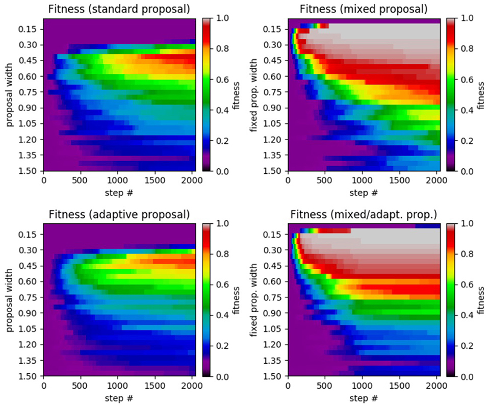
Figure 3. Results of GA test on 5D Ackley function. (Top left) Standard GA. (Top right) Mixed GA. (Bottom left) adaptive GA. (Bottom right) Mixed/adaptive GA. The horizontal axis displays the step number while the vertical axis represents the the proposal width (increases downward). The color axis displays the average fitness across the 20 runs of each method.

We see a similar increase in performance from the standard case to the mixed case as was seen in the SA case. The standard GA case achieved a highest average fitness of 0.9698 at a width of 0.1520 while the mixed case achieved a highest average fitness of 0.9707 at a width of 0.0971. Unlike the SA cases, adaptation did not make significant improvement in performance. Though the adaptive case did achieve a marginally higher average fitness (0.9832) than the standard GA, it did not have the effect of achieving a robust level of performance across a range of widths. Similarly, the mixed/adaptive case merely performs marginally better with a highest average fitness of 0.9764. See Table 1 for a comparison of the peak performance of the various SA and GA methods.

TABLE 1

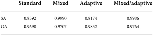
Table 1. Summary of peak average fitness between all four SA and GA cases on the 5D Ackley benchmark problem.

3.1.3. Markov chain Monte Carlo

We now present the results of the IAC and SRF tests on the MCMC implementation of our mixing method in the context of the Ackley benchmark. We compare results from standard Metropolis (MH), mixed Metropolis (MX), adaptive Metropolis (AM), and adaptive-mixed Metropolis (AX). We used identical parameter ranges, mixing amplitudes, and mixing probabilities. The number of steps was set to $N_{step}=2^{11}$ with N_burn = N_step/2. We tested a range of 20 proposal widths with 100 chains generated for each in order to obtain reliable averages. Also, recall that in the Ackley function, all parameters are identical, so we should not see a significant difference in any of the plots of each parameter.

Figure 4 shows the results of the IAC test. Examining any of the five plots, we see that for proposal widths smaller than 2, there is a clear ordering of method performance. In decreasing order we have AX, AM, MX, then MH. For these widths, we see that the mixed methods are superior to their unmixed counterpart. For width values larger than 2, we see that the two mixed methods become poorer than their unmixed counterparts. Both of these phenomena can be explained by the presence of the widening option in the mixing scheme.

FIGURE 4

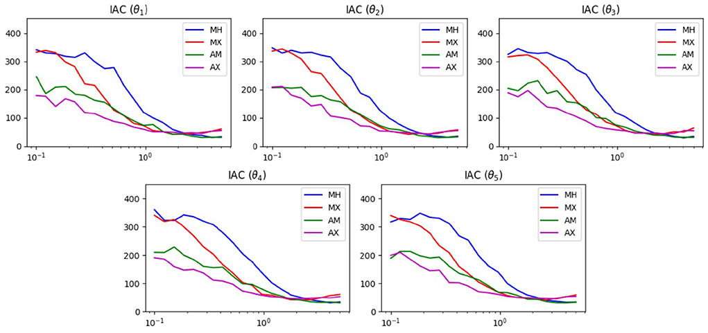
Figure 4. IAC results of MCMC test on the 5D Ackley function. The horizontal axis displays the proposal width (logarithmic scale). The vertical axis is the average lower bound of the IAC.

Figure 5 shows the results of the SRF test. We see similar results in this test as the previous one. For widths below 1, the mixed methods are superior. This is reasonable, since without the widening option, the chain has difficulties escaping the local minima of the Ackley function. Also, for widths >1, all methods achieve roughly the same SRF. At these widths, the chain can already escape the local minima and does not need help from the widened proposal.

FIGURE 5

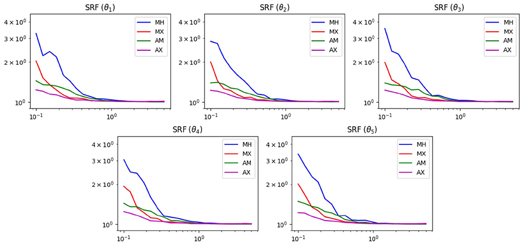
Figure 5. SRF results of MCMC test on the 5D Ackley function. The horizontal axis displays the proposal width (logarithmic scale). The vertical axis is the SRF (logarithmic scale).

3.2. Benchmark 2: Thermal isomerization of α-pinene

For our second benchmark test, we apply our method to the more realistic case of the thermal isomerization of α-pinene (y₁) into dipentene (y₂) and alloocimene (y₃), which then yields α- and β-pyronene (y₄) and a dimer (y₅) [22]. This is a popular benchmark problem that has seen much attention in the literature [23–26]. This is because it suffers significantly from structural non-identifiablility due to certain linear dependencies inherent within the data and model [27].

Assuming first-order kinetics, the ODE's for the system are given by

$\begin{array}{l}{\dot{y}}_1=-({\theta }_1+{\theta }_2)y_1,\\ {\dot{y}}_2={\theta }_1{y}_1,\\ {\dot{y}}_3={\theta }_2{y}_1-({\theta }_3+{\theta }_4)y_3+{\theta }_5{y}_5,\\ {\dot{y}}_4={\theta }_3{y}_3,\\ {\dot{y}}_5={\theta }_4{y}_3-{\theta }_5{y}_5,& (20)\end{array}$

with analytical solutions available in [27]. The data to which the above model must be fit is shown in Table 2 and was obtained by Fuguitt and Hawkins [22], who reported concentrations for the reactant and four products at 8 different times. The best known solution [28] is θ^* = (5.9256·10⁻⁵, 2.9632·10⁻⁵, 2.0450·10⁻⁵, 2.7473·10⁻⁴, 4.0073·10⁻⁵).

TABLE 2

Table 2. Data for α−pinene concentrations from Fuguitt and Hawkins [22].

The most straightforward way to calculate a form of error for this problem would be to simply calculate the sum of squared differences (between the data and the model) in concentration of the chemical species at the given times. Initial testing with this error calculation led to poor convergence, likely due to parameter space being littered with local maxima. Therefore, we instead choose to calculate the sum of squared differences in the derivatives

$\begin{array}{ll}ϵ{(\theta )}^2={\displaystyle \sum _{i=2}^{N_{int-1}}}\left|\right|f(y_i,\theta )-(y_{i+1}-y_{i-1})/(2dt)|{|}^2,& (21)\end{array}$

where dt is the timestep, f is the vectorized right-hand side of Equation (20) and the y_i are linearly interpolated from the data in Table 2. For the SA and GA cases, we calculate fitness via

$\begin{array}{ll}F(\theta )=\left(\frac{1}{1+ϵ{(\theta )}^{1/2}}\right).& (22)\end{array}$

The square root was added from the previous test since the errors can reach up to the order of 10⁵. Squaring and inverting such large number can lead to negligible fitnesses. For the MCMC case, we again used a uniform prior distribution over the entire search space and used the likelihood function

$\begin{array}{ll}\ell (y|\theta )=\text{exp}\left(-\frac{ϵ{(\theta )}^2}{2{\sigma }^2}\right),& (23)\end{array}$

where σ = 15 (again chosen to achieve an acceptance rate of between 0.25 and 0.5).

3.2.1. Simulated annealing

Now, we present the results of the SA test on the α−pinene application (see Figure 6). We again use the 100 samples and 30 proposal width values as in the previous problem. The parameter space is set to θ_m∈[0, 0.2] for m = 1, ⋯ , 5. The mixing amplitudes used were (A_t, A_w) = (1/10, 2) and the mixing probabilities used were (p_t, p_f, p_w) = (0.501253, 0.333333, 0.165414). Since the reaction coefficients which must be estimated are very small, we choose smaller amplitudes than in the Ackley case. Again, both the cooling constant τ and the burn-in time were set to be half the total number of time steps.

FIGURE 6

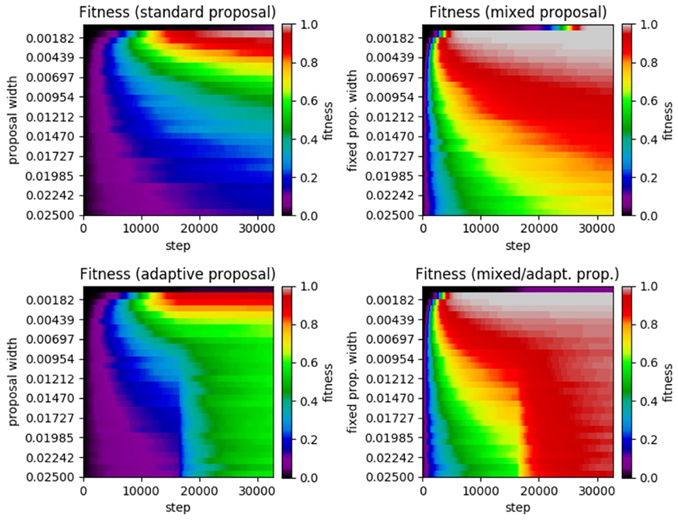
Figure 6. Results of SA test on the α−pinene application. (Top left) Standard SA. (Top right) Mixed SA. (Bottom left) Adaptive SA. (Bottom right) Mixed/adaptive SA. The horizontal axis displays the step number while the vertical axis represents the the proposal width (increases downward). The color axis displays the average fitness across the 100 runs of each method.

Reviewing the plot, we see very similar results to that of the Ackley test. We see that the standard SA achieved a maximum average fitness of 0.9891 at a width of 0.0010 with a significant drop in performance for larger widths. Moving on to the mixed case, the highest average fitness achieved was 0.9999 at a fixed width of 0.0001 (no smaller widths were tested). Like in the previous Ackley test, the mixed method's performance does not decrease as rapidly when widths far from the optimal are chosen. In the adaptive case, the highest average fitness (a value of 0.9136 at a width of 0.0010) was lower than in the standard case, yet it was more robust in that it did not perform as poorly with proposal widths far from the optimal. Lastly, the mixed/adaptive case has a marginaly lower highest average fitness (a value of 0.9994 at a width of 0.0010) than the mixed case. However, it was the most robust by far, consistently achieving high fitness across the entire range of tested proposal widths.

3.2.2. Genetic algorithm

Moving on to the results of the application of GAs to the α−pinene problem, we again have standard GA, mixed GA, adaptive GA, and mixed/adaptive GA. The results are displayed in Figure 7. The parameter space was again set to θ_m∈[0, 1] for m = 1, ⋯ , 5 with 30 randomly initialized instances over 25 different proposal widths. Identical values of the mixing amplitudes, probabilities, and burn-in time were used.

FIGURE 7

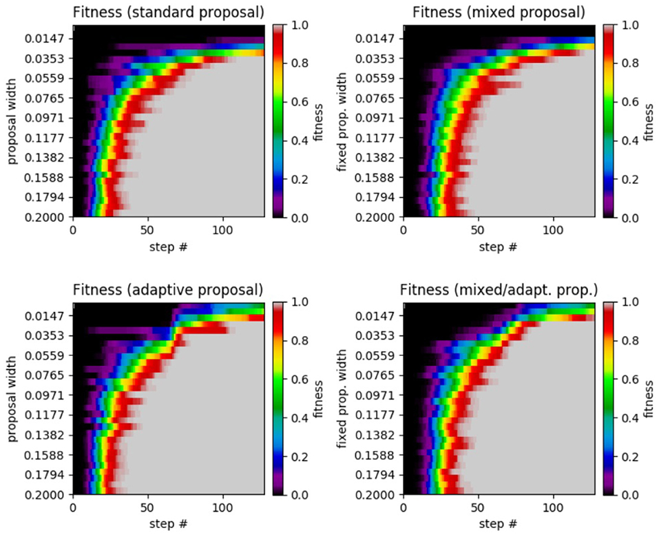
Figure 7. Results of GA test on the α−pinene application. (Top left) Standard GA. (Top right) Mixed GA. (Bottom left) Adaptive GA. (Bottom right) Mixed/adaptive GA. The horizontal axis displays the step number while the vertical axis represents the the proposal width (increases downward). The color axis displays the average fitness across the 25 runs of each method.

The results of this test are unique across all of the experiments we performed since there is very little performance difference between the four different methods (with all methods achieving a fitness of 0.9989 or greater). Perhaps the most noticeable feature of the plots is the superior performance for the adaptive and mixed/adaptive cases (over their non-adaptive counterparts) for very small widths. Table 3 compares the peak performance of the various SA and GA methods on the α−pinene application.

TABLE 3

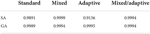
Table 3. Summary of peak average fitness between all four SA and GA cases on the α−pinene application.

3.2.3. Markov chain Monte Carlo

We now present the results of the IAC and SRF tests on the MCMC implementation of our mixing method in the context of the α−pinene problem. We compare results from standard Metropolis (MH), mixed Metropolis (MX), adaptive Metropolis (AM), and adaptive-mixed Metropolis (AX). We used identical parameter ranges, mixing amplitudes, and mixing probabilities. The number of steps was set to $N_{step}=2^{11}$ with N_burn = N_step/2. We tested a range of 20 proposal widths with 100 chains generated for each in order to obtain reliable averages. Also, recall that in the Ackley function, all parameters are identical, so we should not see a significant difference in any of the plots of each parameter.

Figure 8 shows the results of the IAC test. Examining any of the five plots, we see that for proposal widths smaller than 2, there is a clear ordering of method performance. In decreasing order we have AX, AM, MX, then MH. For these widths, we see that the mixed methods are superior to their unmixed counterpart. For width values larger than 2, we see that the two mixed methods become poorer than their unmixed counterparts. Both of these phenomena can be explained by the presence of the widening option in the mixing scheme.

FIGURE 8

Figure 8. IAC results of MCMC test on the α−pinene problem. The horizontal axis displays the proposal width (logarithmic scale). The vertical axis is the average lower bound of the IAC.

Figure 9 shows the results of the SRF test. We see similar results in this test as the previous one. For widths below 1, the mixed methods are superior. This is reasonable, since without the widening option, the chain has difficulties escaping the local minima of the Ackley function. Also, for widths >1, all methods achieve roughly the same SRF. At these widths, the chain can already escape the local minima and does not need help from the widened proposal.

FIGURE 9

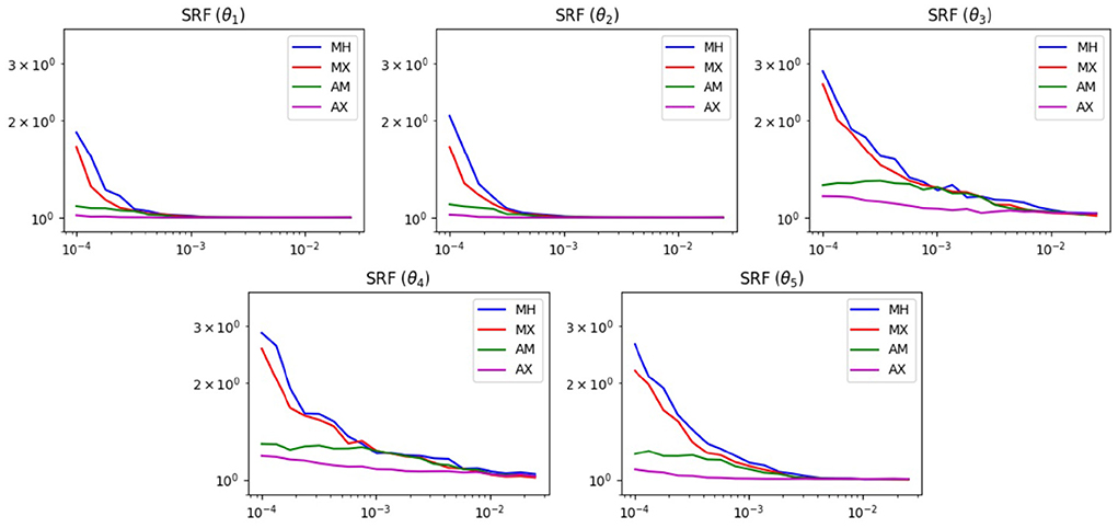
Figure 9. SRF results of MCMC test on the α−pinene problem. The horizontal axis displays the proposal width (logarithmic scale). The vertical axis is the SRF (logarithmic scale).

4. Conclusions

In this paper, we have proposed and tested a Gaussian kernel mixing method that can be easily implemented in a variety of stochastic optimization and Markov chain Monte Carlo contexts. In the majority of test cases, the method served to provide a substantial increase in performance when combined with the chosen base method. Regarding its use in SA, significant improvement was seen in both test problems. Similarly, in the MCMC implementation, our mixed method performed either as well or slightly better than standard Metropolis or AM in both the IAC and SRF tests. For the GA case, improvement was seen in the Ackley test problem. However, in the α−pinene problem, a small reduction in performance was seen. Further testing on more varied types of benchmark functions would be beneficial for determining for which types of problems our mixing method is best suited. Additionally, an extension of the method to beyond three discrete possibilities for mixing should be investigated. More possible mixing amplitudes could be added. Also, a continuous mixing of the form

$\begin{array}{ll}q\left({\theta }^{\prime }|{\theta }^n\right)={\displaystyle {\int }_a^b\rho }\left(A\right)N\left({\theta }^n,{\left(A\sigma \right)}^2\right)dA,& (24)\end{array}$

(with a <1 < b) which preserves the variance σ² would be a reasonable option.

Data availability statement

The original contributions presented in the study are included in the article/supplementary material, further inquiries can be directed to the corresponding author/s.

Author contributions

The idea for the method was developed by GW and JW while working on a separate project. When it was determined that the method might deserve its own paper, ZS was brought onto the project for his expertise in the field. GW was responsible for the coding and testing of the method and all members were involved in the analysis of the results. All authors contributed to the article and approved the submitted version.

Acknowledgments

We would like to thank Middle Tennessee State University, the College of Basic and Applied Sciences, the Computational and Data Sciences Ph.D. Program, and the Department of Mathematics.

Conflict of interest

The authors declare that the research was conducted in the absence of any commercial or financial relationships that could be construed as a potential conflict of interest.

Publisher's note

All claims expressed in this article are solely those of the authors and do not necessarily represent those of their affiliated organizations, or those of the publisher, the editors and the reviewers. Any product that may be evaluated in this article, or claim that may be made by its manufacturer, is not guaranteed or endorsed by the publisher.

References

1. Metropolis N, Rosenbluth AW, Rosenbluth MN, Teller AH, Teller E. Equation of state calculations by fast computing machines. J Chem Phys. (1953) 21:1087–92. doi: 10.1063/1.1699114

CrossRef Full Text | Google Scholar

2. Haario H, Saksman E, Tamminen J. An adaptive metropolis algorithm. Bernoulli. (2001) 7:223–42. doi: 10.2307/3318737

CrossRef Full Text | Google Scholar

3. Hastings WK. Monte Carlo sampling methods using Markov chains and their applications. Biometrika. (1970) 57:97–109. doi: 10.1093/biomet/57.1.97

CrossRef Full Text | Google Scholar

4. Roberts GO, Rosenthal JS. Examples of adaptive MCMC. J Comput Graph Stat. (2012) 18:349–67. doi: 10.1198/jcgs.2009.06134

CrossRef Full Text | Google Scholar

5. Kirkpatrick S, Gelatt CD, Vecchi MP. Optimization by simulated annealing. Science. (1983) 220:671–80. doi: 10.1126/science.220.4598.671

PubMed Abstract | CrossRef Full Text | Google Scholar

6. Aarts EHL, Korst JHM. Simulated annealing and Boltzmann machines - a stochastic approach to combinatorial optimization and neural computing. In: Wiley-Interscience Series in Discrete Mathematics and Optimization. (1990).

Google Scholar

7. Thompson J, Dowsland KA. General cooling schedules for a simulated annealing based timetabling system. In: Edmund KB, Peter R, editors. Practice and Theory of Automated Timetabling. Berlin; Heidelberg: Springer (1996). p. 345–63. doi: 10.1007/3-540-61794-9_70

CrossRef Full Text | Google Scholar

8. Holland JH. Adaptation in Natural and Artificial Systems: An Introductory Analysis with Applications to Biology, Control, and Artificial Intelligence. The MIT Press (1992). doi: 10.7551/mitpress/1090.001.0001

CrossRef Full Text | Google Scholar

9. Pedersen JT, Moult J. Genetic algorithms for protein structure prediction. Curr Opin Struct Biol. (1996) 6:227–31. doi: 10.1016/S0959-440X(96)80079-0

PubMed Abstract | CrossRef Full Text | Google Scholar

10. Montana DJ, Davis L. Training feedforward neural networks using genetic algorithms. In: Proceedings of the 11th International Joint Conference on Artificial Intelligence - Volume 1, IJCAI'89. San Francisco, CA: Morgan Kaufmann Publishers Inc. (1989). p. 762–7.

Google Scholar

11. Meyer TP. Local Forecasting of High-Dimensional Chaotic Dynamics. Addison-Wesley (1992). p. 249–63.

Google Scholar

12. Baker JE. Adaptive selection methods for genetic algorithms. In: ICGA. (1985).

Google Scholar

13. DeJong KA. An Analysis of the Behavior of a Class of Genetic Adaptive Systems (Ph. D. thesis). University of Michigan, Ann Arbor, MI, United States. (1975).

Google Scholar

14. Michalewicz Z. Genetic Algorithms + Data Structures = Evolution Programs. 3rd Edn. Berlin; Heidelberg: Springer (1996). doi: 10.1007/978-3-662-03315-9

CrossRef Full Text | Google Scholar

15. Eshelman LJ, Schaffer JD. Real-coded genetic algorithms and interval-schemata. In: Second Workshop on Foundations of Genetic Algorithms. San Mateo, CA: Morgan Kaufmann Publishers Inc. (1993). p. 187–202. doi: 10.1016/B978-0-08-094832-4.50018-0

CrossRef Full Text | Google Scholar

16. I O, S K. A real-coded genetic algorithm for functional optimization using unimodal normal distribution crossover. In: Proceedings of the 7th International Conference on Genetic Algorithms. East Lansing, MI: Morgan Kaufmann Publishers Inc. (1997). p. 246–53.

Google Scholar

17. Bhandari D, Pal NR, Pal SK. Directed mutation in genetic algorithms. Inform Sci. (1994) 79:251–70. doi: 10.1016/0020-0255(94)90123-6

CrossRef Full Text | Google Scholar

18. Zhou Q, Li Y. Directed variation in evolutionary strategies. IEEE Trans Evol Comput. (2003) 7:356–66. doi: 10.1109/TEVC.2003.812215

CrossRef Full Text | Google Scholar

19. Temby L, Vamplew P, Berry A. Accelerating real valued genetic algorithms using mutation-with-momentum. In: The 18th Australian Joint Conference on Artificial Intelligence. (2005). p. 1108–11. doi: 10.1007/11589990_149

CrossRef Full Text | Google Scholar

20. Solonen A. Proposal adaptation in simulated annealing for continuous optimization problems. Comput Stat. (2013) 10:28. doi: 10.1007/s00180-013-0395-8

CrossRef Full Text | Google Scholar

21. Gelman A, Rubin DB. Inference from iterative simulation using multiple sequences. Stat Sci. (1992) 7:457–72. doi: 10.1214/ss/1177011136

CrossRef Full Text | Google Scholar

22. Fuguitt RE, Hawkins JE. Rate of the thermal isomerization of α-pinene in the liquid phase1. J Am Chem Soc. (1947) 69:319–22. doi: 10.1021/ja01194a047

CrossRef Full Text | Google Scholar

23. Tjoa IB, Biegler LT. Simultaneous solution and optimization strategies for parameter estimation of differential-algebraic equation systems. Indus Eng Chem Res. (1998) 30:376–85. doi: 10.1021/ie00050a015

CrossRef Full Text | Google Scholar

24. Rodriguez-Fernandez M, Egea JA, Banga JP. Novel metaheuristic for parameter estimation in nonlinear dynamic biological systems. BMC Bioinformatics. (2006) 7:483. doi: 10.1186/1471-2105-7-483

PubMed Abstract | CrossRef Full Text | Google Scholar

25. Brunel NJB, Clairon Q. A tracking approach to parameter estimation in linear ordinary differential equations. Electr J Stat. (2015) 9:2903–49. doi: 10.1214/15-EJS1086

PubMed Abstract | CrossRef Full Text | Google Scholar

26. Miro A, Pozo C, Guillen-Gosalbez G, Egea JA, Jimenez L. A tracking approach to parameter estimation in linear ordinary differential equations. BMC Bioinformatics. (2012) 13:90. doi: 10.1186/1471-2105-13-90

PubMed Abstract | CrossRef Full Text | Google Scholar

27. Box GEP, Hunter WG, Macgregor JF, Erjavec J. Some problems associated with the analysis of multiresponse data. Technometrics. (1973) 15:33–51. doi: 10.1080/00401706.1973.10489009

CrossRef Full Text | Google Scholar

28. Egea JA, Rodriguez-Fernandez M, Banga J, Marti R. scatter search for chemical and bio-process optimization. J Global Optim. (2007) 37:481–503. doi: 10.1007/s10898-006-9075-3

PubMed Abstract | CrossRef Full Text | Google Scholar