Early Warning Signals of Financial Crises Using Persistent Homology and Critical Slowing Down: Evidence From Different Correlation Tests

Introduction

Understanding behaviors of financial crises (unexpected and huge declines in the stock market) are crucial to explaining the dynamics of the financial market. However, such financial events are very challenging to study. Among them, the challenges are understanding how the financial market behaves before financial crises and developing a method that is capable to detect early warning signals (EWSs) of the financial crises. The detection method will become more beneficial if it can accurately distinguish the financial market into two classification periods, which are EWS periods (indicating a possible huge downtrend is coming in the market) and safe periods. Such a method helps investors and traders to develop an early precaution strategy and protect their investments from any losses due to a financial crisis.

In practice, the Chicago Board Options Exchange's CBOE Volatility Index or VIX index—a real-time market index representing the market's expectations for volatility over the coming 30 days—is always used by market participants to alert any upcoming financial crisis. The uptrend patterns in the VIX were observed before financial crises, unfortunately, low-level VIX also reported occurred before financial crises [1, 2]. This suggests that the VIX can provide EWSs; however, a reliable method to predict financial crises remains a challenge in this field. Therefore, extensive studies have been conducted by many researchers in an attempt to provide other rationales to explain why financial crises occurred and provide any other possible EWS. Some of those methods are bubble theory [3–5], financial stress indicator [6, 7], information-based measures [8, 9], financial network analysis [10–12], and graphical analysis [13].

However, this study is focusing on critical transition theory. This theory viewed the financial market as a complex system with episodes of critical transitions (abrupt shifts from a current stable state to another stable state when the system reaches critical points) [14, 15]. When approaching a critical point, this theory stated that a generic phenomenon happened known as critical slowing down (CSD) because of decreasing stability in the market and its recovery rate took longer to preserve the stability. At a critical point, the financial market loses its stability in the dynamic state and then suddenly causes a market movement into a financial crisis. CSD gives a rising trend in the time series of some indicators, such as autocorrelation function at lag 1 (AC1), variance (VAR), and mean for power spectrum (MPS) at low frequencies [16–18].

In the traditional method, the rising trend in the time series of CSD indicator that happens before the critical transition point is determined using Kendall's tau correlation test. By using Kendall's tau correlation test, previous studies have shown that the observed rising trend can provide EWSs before financial crises [19–23]. Despite the successful results obtained, there is a realization that some indicator like AC1 also tends to decline before financial crises. All of these lead to mixing results such as recorded in Guttal et al. [21] and Diks et al. [23]. However, as compared to critical transitions, Guttal et al. [21] argued that financial crises are more likely to follow stochastic transition, in which variability indicators (VAR and MPS) can signal early warnings for financial markets. This also points out that abrupt transitions in the financial market are hardly the same as a complex system in nature such as the earth's global climate and interaction between species in ecology. One of the reasons behind this is the financial market is involved with human behaviors that influence the market's movement [23].

Recently, using persistent homology (PH) (a robust method to compute topological features of financial data at different spatial scales [24]), Gidea and Katz [25] suggested a new market representative obtained from persistence landscapes called L¹- norm time series. Since the persistence landscapes are robust under perturbations of the underlying data, the L¹-normtime series has the advantage to reflect the loss of stability in dynamic states of the original system. When the stock market becomes more volatile, loops in the relevant point clouds become much more pronounced and give more significant features within persistence landscapes [25]. At that time, the corresponding L¹-normvalues are more likely to jump up, and this behavior is believed to correspond with an undergoing CSD. Therefore, to test the presence of CSD, the CSD indicators are used with the L¹-normtime series, where these indicators should alert upcoming financial crises by showing their significant rising trend that can be classified by Kendall's tau correlation test. In their work, Gidea and Katz [25] showed that theL¹-normtime series grew substantially before the Dotcom crash and Lehman Brothers bankruptcy in the US market. Interestingly, by using CSD indicators and Kendall's tau correlation test on the L¹-normtime series, Gidea and Katz [25] confirmed that a significant strong rising trend happen in the MPS time series before those two financial crises. Therefore, the method is suggested as a new potential EWS. Later, the application of PH to financial data analysis has attracted more attention from researchers, especially in detecting EWSs. All the articles published in this area are discussed in Section Literature Review.

In this article, we also used PH and CSD indicators (AC1, VAR, and MPS) to detect EWSs of financial crises. Unlike Gidea and Katz [25], instead of using Kendall's tau correlation test to indicate the rising trend in the time series of the indicators, we also examined Pearson's and Spearman's rho correlation tests as a potential substitute for Kendall's tau correlation. The point of comparison between these correlation tests is to determine which test is significant and consistent in classifying the rising trend. The results of such a comparison will suggest the best test that can classify the observed rising trend and detect EWSs of impending financial crises. The remaining portion of this article is organized as follows. Section Literature Review briefly discusses our literature review, Section Persistent Homology introduces PH, Section Data Analysis elaborates on our data, Section Methods presents the applied methods, Section Result mentions our results and their corresponding discussions, and Section Conclusion wraps our conclusion.

Literature Review

Topological information from financial data obtained using PH has been used to study financial problems. In recent times, this topic has attracted attention from many researchers around the globe. In the finance market, the most application currently investigated by PH is financial crises and their EWS detection tools. In a multivariate setting, by begin with examining chaotic time series with noise and a growing variance, Gidea and Katz [25] showed that PH can exhibit strong growth in its market representative time series prior to the critical point. This growth can be analyzed using CSD indicators (AC1, VAR, and MPS) and correlation tests (Kendall's tau) to indicate corresponding CSD that happen before critical point. After that, Gidea and Katz [25] used the pipeline method to examine the Dotcom crash and Lehman Brothers bankruptcy in the US market as mentioned earlier.

After that, Ismail et al. [26] expanded the study of Gidea and Katz [25] by using PH and CSD indicators to examine financial crises in the US, Singapore, and Malaysia markets. Aspects of the method's robustness and prediction performance have been rigorously evaluated in Ismail et al. [26]. Meanwhile, Aromi et al. [27] substantiated that PH reflects changes in the underlying multivariate distribution and strong covariance could nullify the persistence of homologies. On the other hand, [28] also analyzed time-dependent correlation networks using PH to detect early signs of critical transitions in financial data.

In Guo et al. [29], an EWS based on PH is also built to detect the critical dates on the financial time series. Guo et al. [30] also used topological features of complex networks that were extracted using PH to find critical dates for financial crises. In addition, dynamics of financial market correlations based on topology and geometry are examined using PH in Yen et al. [31]. Moreover, Yen and Cheong [32]also tested PH to analyze Singapore and Taiwan markets. The extreme event called flash crash was also explored in Kim et al. [33] by applying PH and dynamic time series analysis.

Furthermore, anomalies detection in the dynamics of a market index also is studied with PH [34]. Katz and Biem [35] also showed that early signatures of growing market instabilities can be captured by PH. Besides, Gidea et al. [3] used PH and k-means clustering to detect critical transitions in the time series of cryptocurrencies. For Bitcoin [36], also uses PH and CSD indicators to detect such transitions and substantiated that PH can detect EWSs better than the detrending time-series approach (the most common approach used in previous studies to detect CSD indicators).

Other than that, PH also has been developed to improve portfolio investment strategies. Studied ten global indices and all their underlying assets, Goel et al. [37] showed that a new strategy based on PH leads to more robust portfolios. Baitinger and Flegel [38] also demonstrated that investment strategies relying on a PH-based turbulence detection outperform investment strategies based on other popular turbulence indices. In clustering and classification of financial time series, Majumdar and Laha [39] showed that PH outperforms other methods in this task.

Additionally, PH is applied with machine learning to predict the movement of financial data. Such a task has been done in Ismail et al. [40] by using PH and machine learning methods (logistic regression, neural network, support vector machine, and random forest) to predict the next-day direction of the Kuala Lumpur Composite Index (KLCI). Moreover, Baitinger and Flegel [41] also introduced PH to produce microstructural predictors, where these predictors are combined with machine learning and statistical factor extraction methods to predict asset returns.

Persistent Homology

Persistent homology is a new quantitative method of topological data analysis to compute topology features (connected components, loops, voids, and others) that persistently emerge across multiple scales. Interestingly, PH is robust to small perturbations of input data, independent of dimensions and coordinates and provides a compact representation of the qualitative features of the input [42–44]. These characteristics make PH suitable to analyze complex, non-linear, noisy, and high-dimensional data like financial data [45].

Later, a summary of PH in the way that it is used in this article is provided. We noted that the concepts of PH stated here can also be found in most books and journals related to PH. To further explore the theories and other concepts of PH, we recommend Otter et al. [24] and Edelsbrunner and Harer [46] to the interested readers.

Input data analyzed by PH is called point cloud dataset (PCD), which can be denoted as $X=\left\{x_i\in {ℝ}^d|i=1,\cdots ,n\right\}$ for d≥2. Let X be a PCD, a Rips complex at a scale ε>0 (denoted as R(X, ε)) can be constructed as follows:

• For each dimensional k = 0, 1, ⋯ , a k-simplex of X points {x_i1, ⋯ , x_i(k+1)} belongs to a R(X, ε) if and only if for every pair {x_ir, x_is}, we have |x_ir−x_is| ≤ ε for all x_ir, x_is∈{x_i1, ⋯ , x_i(k+1) }[24].

Roughly speaking, a Rips complex is a combination of vertices (0-simplex), edges (1-simplex), solid triangles (2-simplex), and higher dimensional analog, joined according to the above-mentioned rule. Figure 1 illustrates 0-simplex until 2-simplex and a two-dimensional Rips complex R(X, ε), respectively. In Figure 1, the scale ε is the diameter of balls around each point in the different PCDs.

FIGURE 1

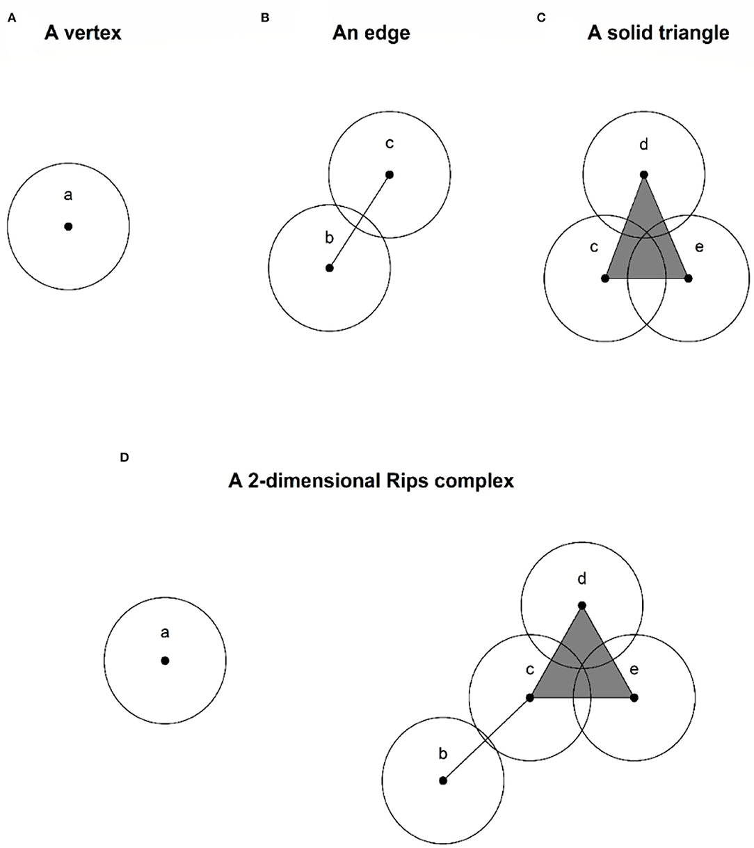
Figure 1. (A,B) are 0-simplex, 1-simplex, 2-simplex, and a two-dimensional Rips complex, respectively.

In a real-world application, finding a single ε is impractical since the real space behind PCD is mostly unknown. Therefore, PH provides a better way to interpret topological information regarding the shape behind PCD by varying the scale ε. Let ε∈{ε₀, ⋯ε_m} such that 0 ≤ ε₀ < ⋯ < ε_m, then filtration of Rips complexes is R(X, ε₀)⊂⋯⊂R(X, ε_m). Figure 2 shows a filtration containing six Rips complexes constructed of a PCD at multiple scales.

FIGURE 2

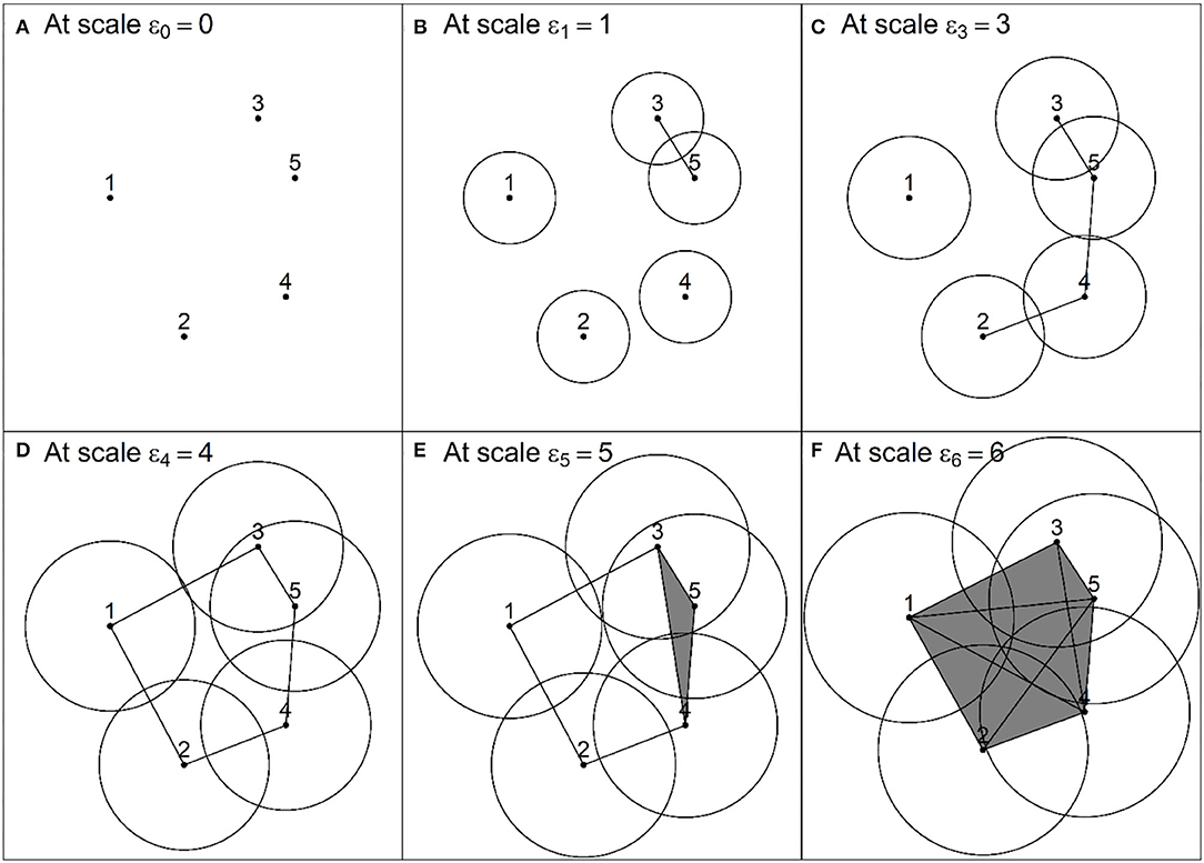
Figure 2. Filtration of six Rips complexes constructed of a PCD at six different scales.

For i = 1, ⋯ , m, we can compute the k-homology of each Rips complex R(X, ε_i), denoted as H_k(R(X, ε_i)). Roughly speaking, H₀(R(X, ε_i)) is the free group generated by the connected components of R(X, ε_i), H₁(R(X, ε_i)) is the free group generated by the loops in R(X, ε_i), H₂(R(X, ε_i)) is the free group generated by the voids of R(X, ε_i). The Betti numbers count the number of generators of such homology groups. This number of generators indicates the number of corresponding topological features that emerge at each scale.

In addition, information regarding the lifespans of topological features also can be obtained by using PH. In the PH community, most believe that a topological feature that has a longer lifespan (persists for a bigger range of scales) can be viewed as a more significant one, whereas a feature that has a shorter lifespan (persists for a smaller range) can be viewed as a less significant, or a noisy feature. Nevertheless, the theoretical justification for this is unclear and may be dependent on the problem at hand [45]. However, this study used all the obtained lifespan in our computation.

Let {(_{εb, εd)i}|i = 1, ⋯ , n} be a collection of the lifespans of topological features such that ε_b < ε_d and ε_b, ε_d∈{ε₀, ⋯ε_m}. The simplest tool to present this information is a persistent barcode, which is a collection of n half-closed intervals [ε_b, ε_d) representing the lifespans of topological features, see Figure 3A. Other tools are a persistent diagram and a persistent landscape. A persistent diagram is a finite collection of n birth–death points $({\epsilon }_b,{\epsilon }_d)\in {ℝ}^2$ that lie along or above a diagonal line. If there are redundant birth–death points, then the points will be represented as a single point but multiplied by its size to correspond to the frequency of this point. Figure 3B provides an example of a persistent diagram.

FIGURE 3

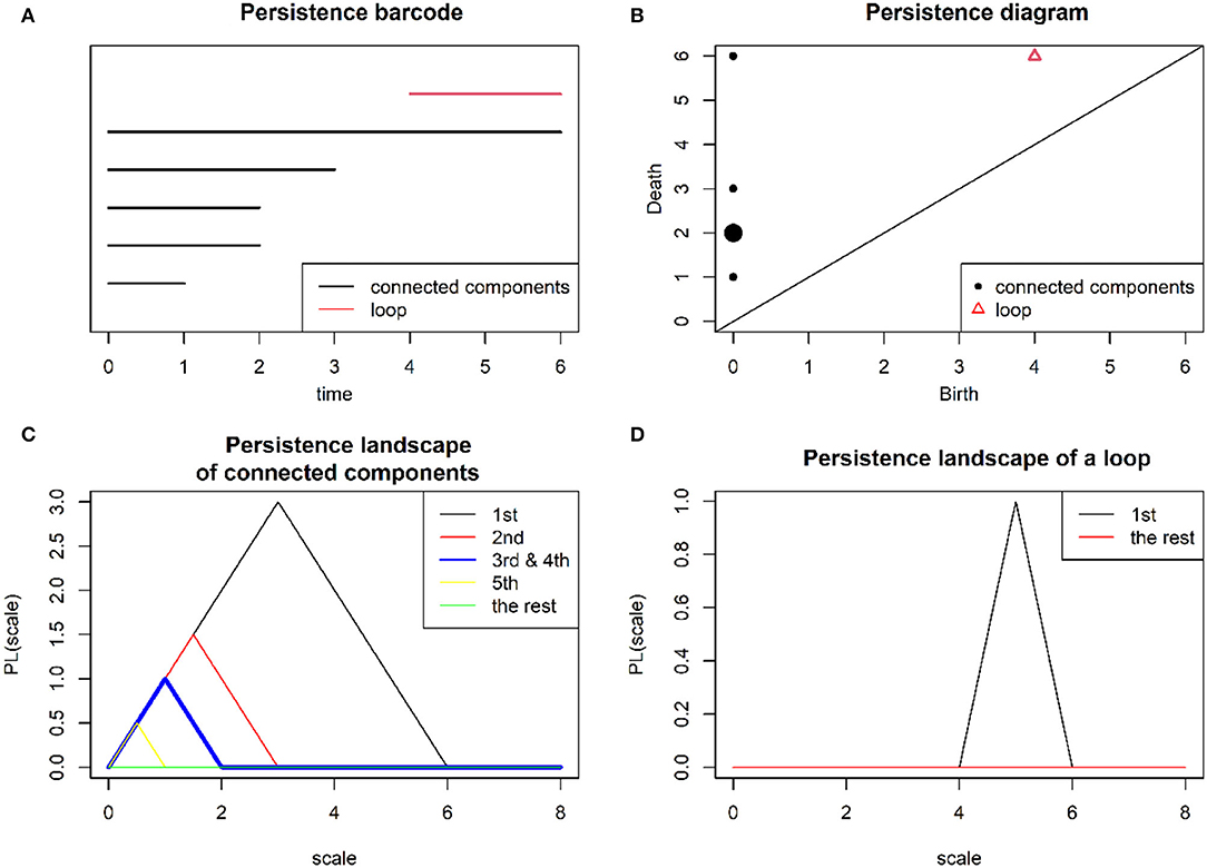
Figure 3. Refer to the filtration of Rips complexes in Figure 2. By applying PH, compact representations: (A) a persistent barcode, (B) a persistence diagram (note that the size for point (0, 2) is enlarged two times bigger than the others to indicate two connected components that share a redundant lifetime), (C) a persistence landscape of connected components (note that the third sub-landscape is enlarged two times bigger than the others to indicate two connected components, which share a redundant lifetime), and (D) a persistence landscape of a loop are obtained.

On the other hand, the persistence landscape λ is quite a recent tool introduced by Bubenik and Dłotko [47] and Bubenik [48]. To define the persistent landscape, we transformed each lifespan into a piecewise linear function f_{(εb, εd)i}: → [0, ∞), which is defined below:

$f_{{({\epsilon }_b,{\epsilon }_d)}_i}(x)=\{\begin{array}{c}x-{\epsilon }_b \text{ if}x\in ({\epsilon }_b,({\epsilon }_b+{\epsilon }_d)/2]\\ -x+{\epsilon }_d \text{ if}x\in (({\epsilon }_b+{\epsilon }_d)/2,{\epsilon }_d)\\ 0 \text{if}x\notin (({\epsilon }_b+{\epsilon }_d))\end{array},$

$\begin{array}{ll}\text{for}i=1,\cdots ,n.& (1)\end{array}$

As a result, we obtained a set of n piecewise linear functions {f_{(εb, εd)i}(x)|i = 1, ⋯ , n}. Later the layer in the persistence landscape was obtained for each k∈ℤ, which is a function λ_k(x):ℝ → [0, ∞)that is defined as follows λ_k(x) = k−max({f_{(εb, εd)i}(x)|i = 1, ⋯ , n}), where k−max denotes the kthlargest value of the piecewise linear functions. If the kth largest value does not exist anymore for k = l, then λ_k(x) = 0for all remaining k≥l. The persistent landscape λ is the infinite sequence of λ_k(x), which can be denoted as {λ₁(x), λ₂(x), ⋯}. Figures 3C,D presents the persistence landscapes of connected components and a loop, respectively.

In this study, we used persistent landscapes because this representation can be summarized into a summary point, that is a L^p-norm. This norm is a function ||.||_p:λ → ℝ, which is defined as follows:

$\begin{array}{ll}{\left|\right|\lambda \left|\right|}_p={\left[{\displaystyle \sum _{k=1}^{\infty }}\int {\left|{\lambda }_k(x)\right|}^{p}dx\right]}^{\frac{1}{p}}\text{for}1\le p<\infty ,& (2)\end{array}$

$\begin{array}{ll}\text{and}{\left|\right|\lambda \left|\right|}_{\infty }{=}_{k,x}^{sup}\left|{\lambda }_k(x)\right|\text{for}p=\infty .& (3)\end{array}$

Furthermore, statistical properties of these norm values also can be analyzed. Therefore, the CSD indicators are computed from these norm values, and they are used to detect EWSs of impending financial crises in this study.

Sample Data

For this study, four main stock indices of the US market were collected, which span from 22/12/1987 until 29/12/2017. The indices were the Standard and Poor's 500 (S&P 500), the Dow Jones Industrial Average (DJIA), the Nasdaq Composite (Nasdaq), and the Russell 2000 Index (Russell 2000), which were derived from the Yahoo Finance. All these indices are shown in Figure 4. In Figure 4, for illustration purposes, the indices are normalized using the max/min normalization using the formula p_norm = 2 × ((p_t−min)/(max−min)), where p_t, max, and min are the closing price at date t, the maximum closing price, and the minimum closing price of an index, respectively. Such normalization does not involve our method as discussed in Section Methods. Furthermore, in Figure 4, the crisis dates for the Dotcom crash and Lehman Brothers bankruptcy are mentioned.

FIGURE 4

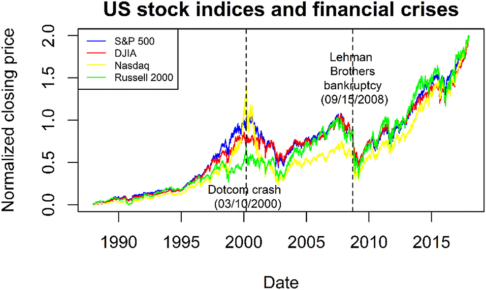
Figure 4. Indices for the Standard and Poor's 500 (S&P 500), the Dow Jones Industrial Average (DJIA), the Nasdaq Composite (Nasdaq), and the Russell 2000 Index (Russell 2000), respectively. The crisis dates for the Dotcom crash and Lehman Brothers bankruptcy also are mentioned.

Methods

Pre-crisis Dataset

In this study, two pre-crisis datasets were generated. The two datasets contained closing prices of the four indices (S&P 500, DJIA, Nasdaq, and Russell 2000) with a length of 1000 before the crisis date of the Dotcom crash and Lehman Brothers bankruptcy, respectively. The objective of creating the two pre-crisis datasets was to study the financial market's behaviors before the financial crises, where the obtained information based on PH and CSD would be proceeded to form a EWS detection. Later, we predicted and compared the performance for the case of using different correlation tests: Kendall's tau, Pearson's, and Spearman's rho.

Persistent Homology

For i = 1, ⋯ , 4, 1000 closing prices of an index i in the pre-crisis were transformed to daily log returns using the formula $r_t^i=ln(p_t^i/p_{t-1}^i)$ for t = 1, ⋯ , 1000, where $p_t^i$ is the closing price at date t. As a result, for each pre-crisis dataset, we obtained a transformed pre-crisis dataset, denoted as $X=\left\{r_t\in {ℝ}^4|t=1,\cdots ,1000\right\},$ where $r_t=(r_t^1,\cdots ,r_t^4)$ is a point of the X at the date t. Xcan be illustrated in matrix form as below:

$\begin{array}{ll}X=\left[\begin{array}{cccc}\begin{array}{c}{r}_1^1\\ r_2^1\\ ⋮\\ r_{1000}^1\end{array}& \begin{array}{c}{r}_1^2\\ r_2^2\\ ⋮\\ r_{1000}^2\end{array}& \begin{array}{c}\cdots \\ \cdots \\ \ddots \\ \cdots \end{array}& \begin{array}{c}{r}_1^4\\ r_2^4\\ ⋮\\ r_{1000}^4\end{array}\end{array}\right]& (4)\end{array}$

Furthermore, the daily sliding window of length 50 approach was applied to segment the X to obtain PCDs. For financial data analysis, it had been demonstrated that a length of 50 was enough to extract topological information through PH as reported in the previous literature reviews [3, 25, 26, 35]. Consequently, each respective PCD from X at the date t also can be illustrated in matrix form as follows:

$\begin{array}{l}X(t)=\left[\begin{array}{cccc}\begin{array}{c}{r}_{((t-50)+1)}^1\\ r_{((t-50)+2)}^1\\ ⋮\\ r_{((t-50)+50)}^1\end{array}& \begin{array}{c}{r}_{((t-50)+1)}^2\\ r_{((t-50)+2)}^2\\ ⋮\\ r_{((t-50)+50)}^2\end{array}& \begin{array}{c}\cdots \\ \cdots \\ \ddots \\ \cdots \end{array}& \begin{array}{c}{r}_{((t-50)+1)}^4\\ r_{((t-50)+2)}^4\\ ⋮\\ r_{((t-50)+50)}^4\end{array}\end{array}\right],\end{array}$

$\begin{array}{ll}\text{for}t=1,\cdots ,1000.& (5)\end{array}$

For each t, as briefed in Section Persistent Homology, PH of Rips filtration that built on PCD X(t), the corresponding persistence landscape at the date t and the corresponding L¹-norm value at the date t were computed, accordingly. By doing so, we obtained L¹-normtime series, denoted by Y = {||λ||_{1, t}|t = 50, ⋯ , 1000}, where ||λ||_{1, t} is a L¹-norm value at the date t.

Critical Slowing Down Indicators

Consequently, the L¹-normtime series Y = {||λ||_{1, t}|t = 50, ⋯ , 1000} was segmented by using the daily sliding window of the length 500 to obtain sequences of 500 L¹-norm values. The length 500 was selected based on the literature mentioned in Guttal et al. [21], Diks et al.[23], and Ismail et al. [ 26], which uses half of the length of the pre-crisis dataset. Each sequence of 500 L¹-norm values at the date t can be denoted as below:

$\begin{array}{l}\text{Y}(t)=\left\{{\left|\right|\lambda \left|\right|}_{1,((t-500)+1)},\cdots ,{\left|\right|\lambda \left|\right|}_{1,((t-500)+500)}\right\},\end{array}$

$\begin{array}{ll}\text{for}t=549,\cdots ,1000.& (6)\end{array}$

For each t∈{549, ⋯ , 1000}, we computed a value based on the CSD indicators: AC1, VAR, and MPS at low frequencies as accordingly defined below:

• The AC1 value at trading t is $ac{1}_t={\rho }_{1,t}{/}_{\mathrm{var}}t,$ where ${\rho }_{1,t}=\frac{1}{500-1}\sum _{j=((t-500)+1)}^{((t-500)+500)-1}({\left|\right|\lambda \left|\right|}_{1,j}-{\overline{\left|\right|\lambda \left|\right|}}_{1,j})({\left|\right|\lambda \left|\right|}_{1,(j+1)}-{\overline{\left|\right|\lambda \left|\right|}}_{1,j}),$ [[Mathtype-mtef1-eqn-106.mtf]] is the mean of Y(t) and var_t is the VAR of Y(t) as defined in the point below.

• The VAR value at the date t is ${var}_t=\frac{1}{500-1}\sum _{j=((t-500)+1)}^{((t-500)+500)-1}{({\left|\right|\lambda \left|\right|}_{1,j}-{\overline{\left|\right|\lambda \left|\right|}}_{1,j})}^2,$ where ${\overline{\left|\right|\lambda \left|\right|}}_{1,j}=\frac{1}{500}\sum _{j=((t-500)+1)}^{((t-500)+500)}{\left|\right|\lambda \left|\right|}_{1,j}$ the mean of Y(t).

• Given Y(t) = {||λ||_{1, ((t−500)+1)}, ⋯ , ||λ||_{1, ((t−500)+500)}}, we defined its discrete Fourier transformation as $F_{k,t}=\sum _{j=((t-500)+1)}^{((t-500)+500)}{\left|\right|\lambda \left|\right|}_{1,j}·e^{{}^{-2\pi ikj}{/}_{500}}$, where k∈{1, ⋯ , 500}. The power spectrum is $P{S}_{k,t}={\left|F_{k,t}\right|}^2$ for k∈{1, ⋯ , 500}. Then, the MPS value at the date t, denoted as mps_t is the mean of all PS_{k, t} for $k\in \left\{2,\cdots {,}^1{/}_8\times 500\right\}$.

As a result, we obtained three sets of time series based on AC1, VAR, and MPS values, which can be denoted as AC1 = {ac1_t|t = 549, ⋯ , 1000}, VAR = {var_t|t = 549, ⋯ , 1000}, and MPS = {mps_t|t = 549, ⋯ , 1000} accordingly.

Correlation Tests

In the study, Kendall's tau correlation was used to determine a rising trend in the indicator's time series (AC1, VAR, or MPS). Nonetheless, Pearson's and Spearman's rho correlations were included in addition to Kendall's tau correlation as alternative measures to detect the trend. In brief, Kendall's tau, Pearson's, and Spearman's rho correlations computed the strength of concordance dependency, the range of linear relationship, and the degree of the association, respectively.

Daily sliding window of length 250 was used to attain sequences containing 125 indicator values. In addition, the length of 250 was chosen as half data of the previous sliding window with length of 500. This length was considered sufficient to capture rising trend in the indicators as shown in Guttal et al. [21] and Ismail et al. [26]. Therefore, three tests based on Kendall's tau, Pearson's, and Spearman's rho correlations from each sequence containing 250 indicator values were computed. Considering AC1 as an example, each sequence containing 250 AC1 values at the date t can be denoted as AC1(t) = {ac1_t|t = ((t−250)+1), ⋯ , ((t−250)+250)}, for t = 798, ⋯ , 1000. For each t∈{798, ⋯ , 1000}, Kendall's tau, Pearson's, and Spearman's rho correlations from AC1(t) are computed as follow:

• ${\tau }_{AC1,t}{=}^{(C-D)}{/}_Z,$ where C is the number of concordant pairs between AC1(t) and {((t−250)+1), ⋯ , ((t−250)+250)}, D is the number of discordant pairs between [[Mathtype-mtef1-eqn-136.mtf]] and {((t−250)+1), ⋯ , ((t−250)+250)}. Z = (250 × (250−1))/2 is the total number of different possible pair combinations.

• $r_{AC1,t}=(250\underset{((t-250)+250)}{\overset{l=((t-250)+1)}{{{\displaystyle \sum }}^{\text{}}}}ac{1}_l·l-(\underset{((t-250)+250)}{\overset{l=((t-250)+1)}{{{\displaystyle \sum }}^{\text{}}}}ac{1}_l)$ $(\underset{((t-250)+250)}{\overset{l=((t-250)+1)}{{{\displaystyle \sum }}^{\text{}}}}l))$ $(\sqrt{250(\underset{((t-250)+250)}{\overset{l=((t-250)+1)}{{{\displaystyle \sum }}^{\text{}}}}{(ac{1}_l)}^2)-{(\underset{((t-250)+250)}{\overset{l=((t-250)+1)}{{{\displaystyle \sum }}^{\text{}}}}ac{1}_l)}^2}$ $\sqrt{250(\underset{((t-250)+250)}{\overset{l=((t-250)+1)}{{{\displaystyle \sum }}^{\text{}}}}{(l)}^2)-{(\underset{((t-250)+250)}{\overset{l=((t-250)+1)}{{{\displaystyle \sum }}^{\text{}}}}l )}^2})$

• $p_{AC1,t}=1-\frac{6\sum _i{d}_i^2}{250({250}^2-1)},$ where d_i is the difference between the ranks of the corresponding variables of AC1(t), and {((t−250)+1), ⋯ , ((t−250)+250) }.

As a result, three sets of time series based on Kendall's tau, Pearson's, and Spearman's rho correlation values computed from AC1 were obtained, which can be denoted as τ_AC1 = {τ_{AC1, t}|t = 798, ⋯ , 1000}, r_AC1 = {r_{AC1, t}|t = 798, ⋯ , 1000}, and p_AC1 = {p_{AC1, t}|t = 798, ⋯ , 1000}., respectively. For, VAR and MPS, the same three sets of time series based on these three correlation values also can be obtained using the above formula.

Note that if any correlation (Kendall's tau, Pearson's, or Spearman's rho) provides a positive real value at the date t, we conclude that a rising trend happened in the 250 indicator values from the date (t−250+1) to t. In critical transition theory, it was expected that these indicators' time series: AC1, VAR, and MPS are increasing before a financial crisis. In addition, the rising trend in the indicators will give rise to a positive real number of the correlation ahead of a financial crisis.

Significant and Skewness Tests

Furthermore, we performed a significance test in this study to examine whether the rising trend in the last 125 indicator values at the date from 750 to 999, which was summarized by the correlation value at the date t = 999 (1 day before the financial crisis), was statistically significant at level 5%. To conduct the test, we computed the p-value for each of the correlation values at the date t = 999. The p-value obtained is a doubled probability of getting the statistical value or a value with even greater evidence against H₀.

Let us take AC1 as an example; here, H₀ represents no monotonic trend (either rising or declining) that happens in the time series AC1(999). A significance test at level 5% translates to a requirement p-value less than 0.005 to interpret any monotonic trend (rising or decline) in the time series AC1(999) as significant or otherwise. The same significant test was also applied to VAR and MPS time series, that is, VAR(999) and MPS(999), respectively. This significance test is vital to verify whether PH via L¹-normtime series associated with the used indicator (AC1, VAR, or MPS) can provide a reliable EWS at least 1 day before the observed financial crisis.

In addition, since the Pearson correlation is usually applied to time series whose probability distribution is symmetric, such as the normal or Gaussian probability distribution, it is better to consider other association correlation measures (Kendall's tau or Spearman's rho) when the probability distribution for the considered time series is asymmetric. Therefore, we also employed the skewness test to observe whether the probability distribution of the last 125 indicator values at the date from 750 to 999 is asymmetric. As a result, we also computed the skewness value for each of the Pearson correlation at the date t = 999.

If the skewness value equals zero, the observed series is perfectly symmetrical. But a skewness of exactly zero is quite unlikely for real-world data, so we interpreted the skewness value as follows:

• If skewness is between −1/2 and 1/2, the distribution can be called approximately symmetric. For this case, the Pearson correlation is applicable to detect EWSs of impending financial crises.

• Otherwise, the distribution is called skewed, and the Pearson correlation is not considered.

Threshold

In this study, by using the test (Kendall's tau, Pearson's, or Spearman's rho correlation), if there exist two significant correlation values, which indicate the significant rising trend in the observed indicator (AC1, VAR, or MPS) 1 day before the two corresponding observed financial crises (Dotcom crash and Lehman Brothers bankruptcy) in the US, a threshold was determined by choosing the smaller value of those two values. Let us assume that T₁ and T₂ are these two thresholds for the US market, then T = min{T₁, T₁} is the threshold covering all available dates. The minimum value was chosen because it corresponded to the most extreme cases, which provided us with the longest period of significant rising trends in the correlation time series (AC1, VAR, and MPS) before the Dotcom crash and Lehman Brothers bankruptcy.

After computing the threshold, all available dates were covered, and the likelihood of an indicative period of significant rising trends, which lay above the threshold, was determined. The latter was made following the range of time at which the indicative trend could be observed. Finally, all the recorded events (periods with significant rising trends and breakpoints or without that signal) were classified either as EWSs, false alarms (FAs), false negatives (FNs), or true negatives (TNs) as described in the later section.

Classification

In our practice, we classified any recorded event (a period with significant rising trends and breakpoints or without that signal) as a EWS, an FA, an FN, or a TN and is as follows:

• If there is a nearest financial crisis that happened within a period of continuous significant rising trends with breakpoints, which lies above the threshold, we consider the event in this period as an EWS.

• If there is no nearest financial crisis that happened within a period of continuous significant rising trends with breakpoints, which lies above the threshold, the event on this period is considered as an FA.

• If there is a financial crisis that happened within a period without the observed signal, which lies below the threshold, we consider the event in this period as an FN.

• If there is no nearest financial crisis within a period without the observed signal, which lies below the threshold, the event in this period is considered as a TN.

Evaluation Measures

For evaluation measures, the classification matrix used in our study is as given in Table 1. To evaluate the method's performance, we used two classification scores (in percentage), namely probability of successful anticipation (PSA) and probability of erroneous anticipation (PEA). These two scores are defined as follows: let A, B, C, and D be the total number of EWS, FA, FN, and TN, respectively, then

$\begin{array}{ll}PSA=((A+D)/(A+B+C+D))\times 100\%& (7)\end{array}$

$\begin{array}{ll}PEA=((B+C)/(A+B+C+D))\times 100\%& (8)\end{array}$

TABLE 1

Table 1. The classification matrix used in this study.

To evaluate, a method that scores the highest PSA and the lowest PEA is considered the best EWS detection tool.

Result

Two pre-crisis datasets were analyzed, whereby each of those datasets had a length of 1,000 days before a financial crisis. In the first row of Figure 5, the two pre-crisis datasets before the Dotcom crash and Lehman Brothers bankruptcy are presented, respectively. For all indices in each pre-crisis dataset, we computed all its corresponding daily log-return time series and then combined all the computed daily log returns to build a high-dimensional time series. Furthermore, the daily sliding window of length 50 was applied to obtain PCDs. Then, we applied PH on each PCD to obtain a corresponding L¹-norm value. As a result, we acquired a L¹- norm time series. All obtained L¹- norm time series for every pre-crisis dataset is illustrated in the second row of Figure 5.

FIGURE 5

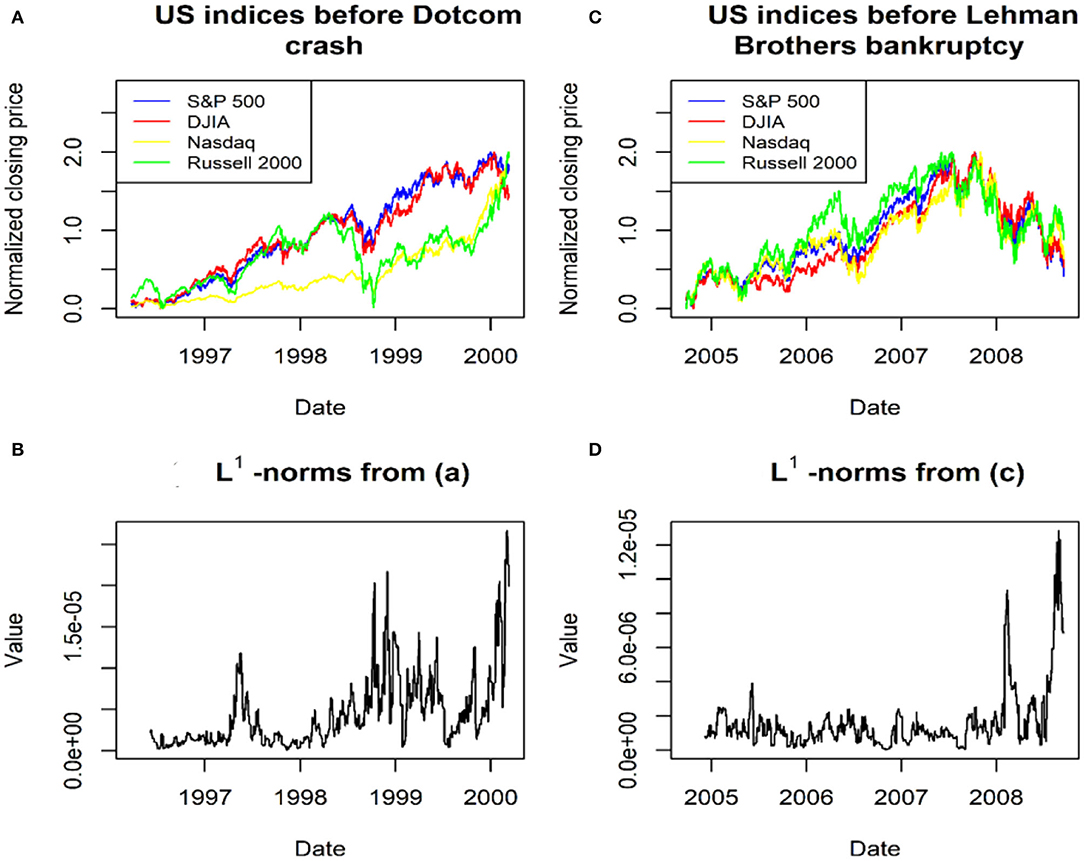
Figure 5. (A,C) two pre-crisis datasets before the Dotcom crash and Lehman Brothers bankruptcy and (B,D) the two L¹-norm time series for these two datasets, respectively.

Figure 5 demonstrates that the L¹-norm time series exhibits strong growth toward a primary peak prior to the Dotcom crash and Lehman Brothers bankruptcy in the US market. These results are consistent with Gidea and Katz [25]and Ismail et al. [26]. As stock indices become increasingly volatile when moving closer to a financial crisis, more peaks appear in its corresponding persistent landscape. The latter gives growth in the L¹-norm values prior to the Dotcom crash and Lehman Brothers bankruptcy [26].

Furthermore, the daily sliding window with the length of 500 was applied to each L¹-norm time series as shown in Figure 5, and the corresponding time series of three CSD indicators, including AC1, VAR, and MPS at low frequencies were obtained. Furthermore, for each computed CSD indicator's time series, we applied the daily sliding window with a length of 250 and computed the time series of three tests: Kendall's tau, Pearson's, and Spearman's rho correlations. In addition, we also employed a significant test to compute p-values for each correlation test 1 day before the Dotcom crash and Lehman Brothers bankruptcy. Figure 6 shows the time series of these CSD indicators (AC1, VAR, and MPS) and presented the obtained value for Kendall's tau, Pearson's, and Spearman's rho correlations before the financial crises. Moreover, in Figure 6, corresponding p-values for Kendall's tau, Pearson's, and Spearman's rho correlations and skewness measure (for the Pearson correlation only) are also mentioned. Kendall's tau correlation, Pearson's correlation, Spearman's rho correlation, p-values for Kendall's tau correlation, p-values for Pearson's correlation, p-values for Spearman's rho correlation, and skewness values in Figure 6 are symbolized with τ, r, p, p_τ, p_r, p_p, and s, respectively.

FIGURE 6

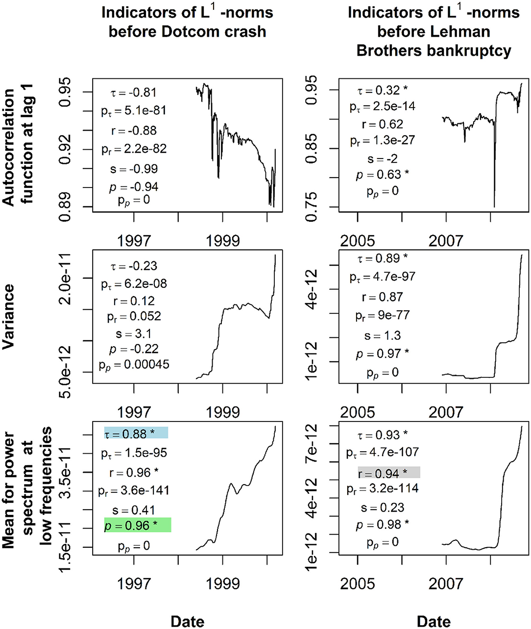
Figure 6. Time series of the CSD indicators (AC1, VAR, and MPS), the obtained value for Kendall's tau, Pearson's, and Spearman's rho correlations, and their corresponding p-values 1 day before the financial crises.

Based on the results presented in Figure 6, for any CSD indicator of the L¹-normtime series, which consistently exhibits a significant rising trend (indicated by the correlation values, the corresponding p-values, and skewness) before the observed financial crises, we considered such method as a EWS detection tool. It is clearly shown that only the MPS time series of the L¹-norm time series fulfill this condition, and its significant rising trend can be indicated by Kendall tau, Pearson, and Spearman rho correlation. These because Kendall tau and Spearman rho provide positive values and their corresponding p-values also less than 0.05. For Pearson, this test obtains a positive value, its corresponding p-values is less than 0.05, and its skewness values lie in between −1/2 and 1/2 indicating that the data has an approximately symmetrical distribution. For the others, they did not achieve the above-mentioned characteristics, therefore not considered as potential EWS detection tools.

In Figure 6, the highlighted values from different correlation tests (Kendall's tau, Pearson's, and Spearman's rho) are the chosen threshold to predict the whole available date. These values are 0.88, 0.94, and 0.96 for Kendall's tau, Pearson's, and Spearman's rho correlations, respectively. Therefore, we have three predictions performed using three different correlations, and each correlation is obtained from the MPS time series of the L¹-normtime series. For each prediction, all individual events (periods of continuous significant rising trends or otherwise) are recorded, and these events are then classified whether they are EWSs, FAs, FNs, or TNs.

Results obtained from MPS of the L¹-normtime series using Kendall's tau, Pearson's, and Spearman's rho correlations, respectively, are illustrated in Figure 7. All periods of continuous significant rising trends in Figure 7 are indicated by blue numbers and lines, which lie above the threshold. In contrast, correlation values that lie below the threshold are indicated with black numbers and lines. Details on these recorded events and their corresponding classification as shown in Figure 7 for Kendall's tau, Pearson's, and Spearman's rho correlations are provided in tables of Supplementary Material File.

FIGURE 7

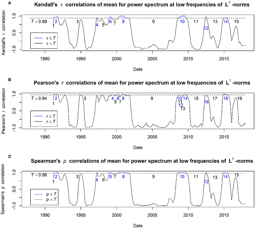
Figure 7. Results obtained from MPS of the L¹-norm time series using Kendall's tau, Pearson's, and Spearman's rho correlations. (A) Kendall's tau correlations of mean for power spectrum at low frequencies of L¹-norms; (B) Pearson's rho correlations of mean for power spectrum at low frequencies of L¹-norms; (C) Spearman's rho correlations of mean for power spectrum at low frequencies of L¹-norms.

By using MPS of the L¹-norm time series, our results reported that Spearman's rho correlation test obtained the total number of EWS, FA, FN, TN, PSA, and PEA of 4, 7, 7, 8, 46.15, and 53.85%, respectively. Furthermore, Kendall's tau correlation test provided the total number of EWS, FA, FN, TN, PSA, and PEA of 3, 8, 7, 8, 42.31, and 57.69%, respectively. In addition, the Pearson correlation test achieved the total number of EWS, FA, FN, TN, PSA, and PEA of 2, 9, 9, 10, 40, and 60%, respectively. All these results obtained are summarized in Table 2, where all the bolded values represent the obtained highest scores for the corresponding evaluation measure.

TABLE 2

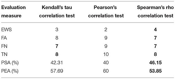
Table 2. A summary for all obtained results.

From Table 2, based on PSA and PEA, Spearman's rho and Kendall's tau correlations are showed to obtain a better result than the Pearson correlation. This shows that non-parametric rank correlation, which computes statistical associations based on the ranks of the data like Spearman's rho and Kendall's tau correlations is better than the Pearson correlation, which measures the degree of the linear relationship between related variables. However, Spearman's rho correlation, which measures the degree of association between two variables is reported and has a better result as compared to Kendall's tau correlation, which measures the strength of dependence between two variables. In addition, our result in Table 2 clearly shows that Spearman's rho correlation outperforms other correlation tests (Kendall's tau and Pearson's correlations) with the highest score of every evaluation measure. Therefore, by using MPS of the L¹-norm time series, our results concluded that Spearman's rho correlation can detect EWSs better than Kendall's tau and Pearson's correlations.

Conclusion

In this study, PH and CSD were proposed to detect EWSs of major financial crashes in the US market. Preliminarily, two financial crises: Dotcom Crash and Lehman Brothers Bankruptcy that happened in the US market were examined. By using PH, L¹-norm time series was obtained for each financial crisis and used to compute the CSD indicators: AC1, VAR, and MPS.

By using three different correlation tests, Kendall's tau, Pearson's, and Spearman's rho, the rising trend in these indicators is observed prior to the financial crises. Furthermore, this study applied significance and skewness tests to determine whether the rising trends in the indicators (AC1, VAR, or MPS) are statistically significant. This test aims to conclude that the rising trend does not happen by chance. Subsequently, a threshold is determined to predict the whole date, and then the classification performance of our method is evaluated by using PSA and PEA.

Our result shows that the L¹-norm time series exhibits a strong growth before Dotcom Crash and Lehman Brothers Bankruptcy. This portrays that the L¹-norm time series has the potential to be a representative to detect EWSs of major financial crashes in the US market. Moreover, MPS from the L¹-norm time series is significantly rising before these two financial crises. It has also been demonstrated that all correlation tests, Kendall's tau, Pearson's, and Spearman's rho, can indicate the observed significant rising trend.

Overall, based on PSA and PEA, our results revealed that Spearman's rho correlation predicts the US market better than Kendall's tau and Pearson's correlations. Therefore, this study demonstrates that PH via its L¹-norm time series with MPS and Spearman's rho correlation offers a new potential EWS detection tool for financial crises in the US market. For future studies, we plan to examine and refine this method of PH to provide more reliable EWSs for upcoming financial crises.

Data Availability Statement

Publicly available datasets were analyzed in this study. This data can be found here: https://finance.yahoo.com

Author Contributions

MSI: conceptualization, methodology, software, validation, writing–original draft, and writing–review and editing. MM: conceptualization, supervision, validation, writing–review and editing, and funding acquisition. MI: supervision, data curation, validation, writing–review and editing, funding acquisition. FA: supervision, validation, writing–review and editing. All authors contributed to the article and approved the submitted version.

Conflict of Interest

The authors declare that the research was conducted in the absence of any commercial or financial relationships that could be construed as a potential conflict of interest.

The handling editor MM declared a past collaboration with the authors.

Publisher's Note

All claims expressed in this article are solely those of the authors and do not necessarily represent those of their affiliated organizations, or those of the publisher, the editors and the reviewers. Any product that may be evaluated in this article, or claim that may be made by its manufacturer, is not guaranteed or endorsed by the publisher.

Acknowledgments

We would like to express our gratitude to the Universiti Kebangsaan Malaysia and the Ministry of Higher Education Malaysia for their financial support via the provision of two grants with numbers: FRGS/1/2019/STG06/UKM/01/3 and GUP-2020-032.

Supplementary Material

The Supplementary Material for this article can be found online at: https://www.frontiersin.org/articles/10.3389/fams.2022.940133/full#supplementary-material

References

1. D.S. Bates. Jumps and stochastic volatility: exchange rate processes implicit in deutsche mark options. Rev Financ Stud. (2015) 9:69–107. doi: 10.1093/rfs/9.1.69

CrossRef Full Text

2. Gopalakrishnan EA, Sharma Y, John T, Dutta PS, Sujith RI. Early warning signals for critical transitions in a thermoacoustic system. Sci Rep. (2016) 6:35310. doi: 10.1038/srep35310

PubMed Abstract | CrossRef Full Text | Google Scholar

3. Gidea M, Goldsmith D, Katz Y, Roldan P, Shmalo Y. Topological recognition of critical transitions in time series of cryptocurrencies. Physica A Stat Mech Appl. (2020) 548:123843. doi: 10.1016/j.physa.2019.123843

CrossRef Full Text | Google Scholar

4. Virtanen T, Tölö E, Virén M, Taipalus K. Can bubble theory foresee banking crises? J Financial Stab. (2018) 36:66–81. doi: 10.1016/j.jfs.2018.02.008

CrossRef Full Text | Google Scholar

5. Sornette D, Cauwels P. Financial bubbles: mechanisms and diagnostics. Swiss Finance Institute Research Paper. (2014). doi: 10.2139/ssrn.2423790

CrossRef Full Text | Google Scholar

6. H.J. Edison. Do indicators of financial crises work? An evaluation of an early warning system. Int J Finance Econ. (2003) 8:11–53. doi: 10.1002/ijfe.197

CrossRef Full Text | Google Scholar

7. Hubrich K, Tetlow RJ. Financial stress and economic dynamics: The transmission of crises. J Monet Econ. (2015) 70:100–15. doi: 10.1016/j.jmoneco.2014.09.005

CrossRef Full Text | Google Scholar

8. Quax R, Kandhai D, Sloot P. Information dissipation as an early-warning signal for the Lehman Brothers collapse in financial time series. Sci Rep. (2013) 3:1–7. doi: 10.1038/srep01898

PubMed Abstract | CrossRef Full Text | Google Scholar

9. Gatfaoui H, Peretti PDe. Flickering in information spreading precedes critical transitions in financial markets. Sci Rep. (2019) 9:1–11. doi: 10.1038/s41598-019-42223-9

PubMed Abstract | CrossRef Full Text | Google Scholar

10. Squartini T, Van Lelyveld I, Garlaschelli D. Early-warning signals of topological collapse in interbank networks. Sci Rep. (2013) 3:1–9. doi: 10.1038/srep03357

PubMed Abstract | CrossRef Full Text | Google Scholar

11. Saracco F, Clemente RDi, Gabrielli A, Squartini T. Detecting early signs of the 2007–2008 crisis in the world trade. Sci Rep. (2016) 6:1–11. doi: 10.1038/srep30286

PubMed Abstract | CrossRef Full Text | Google Scholar

12. Almog A, Shmueli E. Structural entropy: monitoring correlation-based networks over time with application to financial markets. Sci Rep. (2019) 9:1–13. doi: 10.1038/s41598-019-47210-8

PubMed Abstract | CrossRef Full Text | Google Scholar

13. Flood MD, Lemieux VL, Varga M, Wong BW. The application of visual analytics to financial stability monitoring. J Financial Stab. (2016) 27:180–97. doi: 10.1016/j.jfs.2016.01.006

CrossRef Full Text | Google Scholar

14. Battiston S, Farmer JD, Flache A, Garlaschelli D, Haldane AG, Heesterbeek H, et al. Complexity theory and financial regulation. Science. (2016) 351:818–9. doi: 10.1126/science.aad0299

PubMed Abstract | CrossRef Full Text | Google Scholar

15. D. Sornette Why Stock Markets Crash: Critical Events in Complex Financial Systems. Princeton: University Press (2017). doi: 10.23943/princeton/9780691175959.001.0001

CrossRef Full Text | Google Scholar

16. Van Nes EH, Scheffer M. Slow recovery from perturbations as a generic indicator of a nearby catastrophic shift. Am Nat. (2007) 169:738–47. doi: 10.1086/516845

PubMed Abstract | CrossRef Full Text | Google Scholar

17. Dakos V, Carpenter SR, Brock WA, Ellison AM, Guttal V, Ives AR, et al. Methods for detecting early warnings of critical transitions in time series illustrated using simulated ecological data. PLoS ONE. (2012) 7:e41010. doi: 10.1371/journal.pone.0041010

PubMed Abstract | CrossRef Full Text | Google Scholar

18. Veraart AJ, Faassen EJ, Dakos V, van Nes EH, Lürling M, Scheffer M. Recovery rates reflect distance to a tipping point in a living system. Nature. (2012) 481:357–9. doi: 10.1038/nature10723

PubMed Abstract | CrossRef Full Text | Google Scholar

19. Tan JPL, Cheong SSA. Critical slowing down associated with regime shifts in the US housing market. Eur Phys J B. (2014) 87:1–10. doi: 10.1140/epjb/e2014-41038-1

CrossRef Full Text | Google Scholar

20. Tan J, Cheong SA. The regime shift associated with the 2004–2008 US housing market bubble. PLoS ONE. (2016) 11:e0162140. doi: 10.1371/journal.pone.0162140

PubMed Abstract | CrossRef Full Text | Google Scholar

21. Guttal V, Raghavendra S, Goel N, Hoarau Q. Lack of critical slowing down suggests that financial meltdowns are not critical transitions, yet rising variability could signal systemic risk. PLoS ONE. (2016) 11:e0144198. doi: 10.1371/journal.pone.0144198

PubMed Abstract | CrossRef Full Text | Google Scholar

22. Wen H, Ciamarra MP, Cheong SA. How one might miss early warning signals of critical transitions in time series data: A systematic study of two major currency pairs. PLoS ONE. (2018) 13:e0191439. doi: 10.1371/journal.pone.0191439

PubMed Abstract | CrossRef Full Text | Google Scholar

23. Diks C, Hommes C, Wang J. Critical slowing down as an early warning signal for financial crises? Empir Econ. (2019) 57:1201–28. doi: 10.1007/s00181-018-1527-3

CrossRef Full Text | Google Scholar

24. Otter N, Porter MA, Tillmann U, Grindrod P, Harrington HA. A roadmap for the computation of persistent homology. EPJ Data Science. (2017) 6:1–38. doi: 10.1140/epjds/s13688-017-0109-5

PubMed Abstract | CrossRef Full Text | Google Scholar

25. Gidea M, Katz Y. Topological data analysis of financial time series: Landscapes of crashes. Phys A Stat Mech Appl. (2018) 491:820–34. doi: 10.1016/j.physa.2017.09.028

CrossRef Full Text | Google Scholar

26. Ismail MS, Noorani MSM, Ismail M, Razak FA, Alias MA. Early warning signals of financial crises using persistent homology. Phys A Stat Mech Appl. (2022) 586:126459. doi: 10.1016/j.physa.2021.126459

CrossRef Full Text | Google Scholar

27. Aromi LL, Katz YA, Vives J. Topological features of multivariate distributions: Dependency on the covariance matrix. Commun Nonlinear Sci Numer Simuls. (2021) 103:105996. doi: 10.1016/j.cnsns.2021.105996

CrossRef Full Text | Google Scholar

28. M. Gidea, Topological Data Analysis of Critical Transitions in Financial Networks. In: Shmueli E, Barzel B, Puzis R, (Eds.), 3rd International Winter School and Conference on Network Science. Cham: Springer International Publishing (2017). pp. 47–59. doi: 10.1007/978-3-319-55471-6_5

CrossRef Full Text | Google Scholar

29. Guo H, Xia S, An Q, Zhang X, Sun W, Zhao X. Empirical study of financial crises based on topological data analysis. Phys A Stat Mech Appl. (2020) 558:124956. doi: 10.1016/j.physa.2020.124956

CrossRef Full Text | Google Scholar

30. Guo H, Zhao X, Yu H, Zhang X. Analysis of global stock markets' connections with emphasis on the impact of COVID-19. Phys A Stat Mech Appl. (2021) 569:125774. doi: 10.1016/j.physa.2021.125774

CrossRef Full Text | Google Scholar

31. Yen PT, Xia K, Cheong SA. Understanding changes in the topology and geometry of financial market correlations during a market crash. Entropy. (2021) 23:1211. doi: 10.3390/e23091211

PubMed Abstract | CrossRef Full Text | Google Scholar

32. Yen PT, Cheong SA. Using Topological Data Analysis (TDA) and persistent homology to analyze the stock markets in Singapore and Taiwan. Front Physics. (2021) 9:20. doi: 10.3389/fphy.2021.572216

CrossRef Full Text | Google Scholar

33. Kim W, Kim Y-J, Lee G, Kook W. Investigation of flash crash via topological data analysis. Topol Appl. (2021) 301:107523. doi: 10.1016/j.topol.2020.107523

CrossRef Full Text | Google Scholar

34. Nguyen NKK, Bui M. Detecting anomalies in the dynamics of a market index with topological data analysis. Int J Syst Innovation. (2021) 6:37–50.

Google Scholar

35. Katz YA, Biem A. Time-resolved topological data analysis of market instabilities. Phys A Stat Mech Appl. (2021) 571:125816. doi: 10.1016/j.physa.2021.125816

CrossRef Full Text | Google Scholar

36. Ismail MS, Hussain SI, Noorani MSM. Detecting early warning signals of major financial crashes in bitcoin using persistent homology. IEEE Access. (2020) 8:202042–57. doi: 10.1109/ACCESS.2020.3036370

CrossRef Full Text | Google Scholar

37. Goel A, Pasricha P, Mehra A. Topological data analysis in investment decisions. Expert Syst Appl. (2020) 147:113222. doi: 10.1016/j.eswa.2020.113222

CrossRef Full Text | Google Scholar

38. Baitinger E, Flegel S. The better turbulence index? Forecasting adverse financial markets regimes with persistent homology. Financ Mark Portf Manag. (2021) 35:277–308. doi: 10.1007/s11408-020-00377-x

CrossRef Full Text | Google Scholar

39. Majumdar S, Laha AK. Clustering and classification of time series using topological data analysis with applications to finance. Expert Syst Appl. (2020) 162:113868. doi: 10.1016/j.eswa.2020.113868

CrossRef Full Text | Google Scholar

40. Ismail MS, Md Noorani MS, Ismail M, Abdul Razak F, Alias MA. Predicting next day direction of stock price movement using machine learning methods with persistent homology: Evidence from Kuala Lumpur Stock Exchange. Appl Soft Comput. (2020) 93:106422. doi: 10.1016/j.asoc.2020.106422

CrossRef Full Text | Google Scholar

41. E. Baitinger, and S. Flegel, New Concepts in Financial Forecasting: Network-Based Information, Topological Data Analysis and their Combination. (2021). doi: 10.2139/ssrn.3962148

CrossRef Full Text | Google Scholar

42. V. Robins, Towards computing homology from finite approximations. J Adv Stud Topol. (1999) 24: 503–32. Available online at: http://topology.nipissingu.ca/tp/reprints/v24/tp24222.pdf

Google Scholar

43. Edelsbrunner H, Letscher D, Zomorodian A. Topological persistence and simplification. In: Proceedings 41st Annual Symposium on Foundations of Computer Science. New York, NY: IEEE (2000). p. 454–63.

Google Scholar

44. Zomorodian A, Carlsson G. Computing persistent homology. Discrete Comput Geom. (2005) 33:249–74. doi: 10.1007/s00454-004-1146-y

CrossRef Full Text | Google Scholar

45. G. Carlsson. Topology and data. Bull New Ser Am Math Soc. (2009) 46:255–308. doi: 10.1090/S0273-0979-09-01249-X

CrossRef Full Text | Google Scholar

46. Edelsbrunner H, Harer JL Computational Topology: An Introduction. American Mathematical Society(2022).

Google Scholar

47. Bubenik P, Dłotko P. A persistence landscapes toolbox for topological statistics. J Symb Comput. (2017) 78:91–114. doi: 10.1016/j.jsc.2016.03.009

CrossRef Full Text | Google Scholar

48. Bubenik P. Statistical topological data analysis using persistence landscapes. J Mach Learn Res. (2015) 16:77–102. doi: 10.48550/arXiv.1207.6437

PubMed Abstract | CrossRef Full Text | Google Scholar