A unified framework for analyzing complex systems: Juxtaposing the (Kernel) PCA method and graph theory

1. Introduction

Complex systems, a common framework for scientific studies of phenomena composed of more than one entity, stand as a prominent framework of scientific computing. It is hard to think of single phenomenon which do not involve a number of interacting entities.

The notion of network modeling lies in the heart of systems science, providing a solid framework for the study of systems of many interacting entities, requiring no central control. In a network, simple rules of operation can give rise to sophisticated information processing, and adaptation via learning or evolution [1]. A network or a graph [2] can be used to represent any system of a set of entities (consisting of the nodes of the graph) that may be related to each other via pairwise relationships (constituting the edges of the graph). The entities could be any set; a set of atoms, brain centers, molecules, humans, societies, machines, brain centers, countries, planets, stars, or galaxies. The edges are pairwise relations that may declare dependency among the involved entities, conflict, binding, allocation, assignment, (dis)-similarity, friendship, positive or negative relationship, etc. Despite its simple definition, networks and network science have become one of the most powerful interdisciplinary frameworks for the study of complex systems. The strong mathematical foundation of graph theory supports the core of network science while its flexibility and generality make it adaptable to applications in a wide and diverse range of domains of knowledge.

Defining what the nodes and the edges of a graph correspond to in the real system is a crucial step and can be a deceptively challenging task. For more details about structure/function relationships, emerging properties and other factors playing a critical role in the description of complex systems refer to Turnbull et al. [3].

In this work, we present a unified framework for analyzing complex systems and apply it to problems in two diverse fields: neuroscience and astrophysics. The framework brings together different approaches for the analysis of a complex system, i.e., principal component analysis (PCA) and graph theory, under common ground. It provides a number of different computational paths for the analysis of complex systems which enables the juxtaposition of each of them. It also allows different visualization of the core elements of the system, revealing different aspects of it (physical properties or similarities, etc.).

In particular, the framework consists of the following steps: (i) the modeling of the data set as a system in a concrete mathematical form leading to a matrix representation (i.e., a similarity matrix), (ii) The representation of the system either as a graph or as a set of features in space of few dimensions, where (some of the original) metric properties are preserved. These reduced representations provide a fundamental skeleton that captures the most intrinsic and hidden properties of the system. (iii) The application of several kinds of clustering algorithms either directly on the graph or in the reduced feature space, and finally, (iv) The application of various embeddings of the clustered data in the reduced space or using the graph. The embeddings allow both the comparison of the cluster data with other physical properties, the extraction of the most important features of the data set, possible embeddings of new data in the feature space, and the interpretation of the results with the use of domain knowledge. Overall, the framework allows the clarification of the underlying mechanisms and processes within each scientific domain. It can also unveil hidden theoretical similarities in the description of complex systems that can guide the quest for a better overall understanding of each individual system and highlight global patterns that run across scientific domains.

The applicability of the framework is demonstrated in the study of two distinct and apparently very different complex systems, each one affording clear definitions of the nodes and edges at distinct spatial and temporal scales. The first system comes from the domain of neuroscience with structural elements on the large spatial scale of the entire brain, with constituent parts of the cytoarchitectonic areas (CA) [4] on the cortical mantle and other areas in the deep brain nuclei. Two neuroscience problems are addressed, each one as a problems of clustering of functional data from a number of CAs. The first one probes the organization of sleep, where the framework is utilized to characterize the relationship between sleep stages and accommodate the periods of high activity within each sleep stage and periods representing transitions between them. For the second neuroscience application, the framework is applied to probe the nature of evoked responses and the way the thalamus and cortex influence each other. The second system where the framework is applied deals with problems in astrophysics, where galaxies are the nodes. In particular, we study the evolution of ultraluminous infrared galaxies (ULIRGs), through the study of their spectral energy distributions (SEDs). The framework is employed here for the detection of galaxies of similar SEDs which correspond to different galaxy evolution stages, and for the investigation of the relation between various physical properties of the galaxies and in relation to their SEDs.

1.1. Roadmap

In Section 2, we first introduce the theoretical background we use and then present the proposed framework. The first two subsections of Section 2 introduce the related theory and methods of the PCA together with one of its non-linear extensions (Section 2.1) and graph theory (Section 2.2). The following Section 2.3 presents and discusses the proposed framework. Section 2.4 introduces two specific extensions of the framework which are used to produce good effect in the applications of neuroscience. The applicability of the framework is demonstrated in Section 3, where it is successfully applied to the analysis of two distinct complex systems in Neuroscience (Section 3.1) and a problem in Astrophysics (Section 3.2). The article concludes with Section 4 where we summarize the proposed framework, its advantages, and its applicability in diverse sciences.

2. Mathematical framework and methods

2.1. Principal components analysis: Background and methods

Dimension Reduction (DR) techniques provide a mapping of the original data into a lower dimensional space which maintains its main features. PCA is the prototypical dimensionality reduction method, with applications in data clustering, pattern recognition, image analysis, etc. [5, 6]. It is a linear method with the data spread in a Euclidean space of N dimensions that yields an appropriate low-dimensional orthogonal coordinate system with axes defining the direction of the principal variances of the data.

Due to its limited applicability to linearly structured data, various extensions of PCA have been developed in order to cover data with non-linear dependencies [see [5, 7]]. Non-linear DR techniques can deal with highly complex data by assuming that the data lies on a highly non-linear manifold that can be described in a linear space of much lower dimensions than that of linear PCA. In this study, we will also explore a common non-linear dimension reduction technique, the Kernel PCA method [8].

2.1.1. Linear PCA

Assume a set of data of N elements in a D−dimensional Euclidean space, called Input space, represented by N column vectors x_i, i ∈ [N] ¹, each of dimension D, constituting the D × N matrix X. For technical reasons, we consider centered initial data by subtracting the average vector μ² from the data obtaining the new variables ${\overline{\text{x}}}_i={\text{x}}_i-\mu$ and the corresponding matrix $\overline{X}$.

The principal component analysis method attempts to project optimally³. the data points onto a linear subspace (affine subspace in the case of uncentered raw data) of ℝ^D of dimension d (usually d << D), which reduces the eigenvalue decomposition of the D × D matrix $\text{S}=\overline{\text{X}}{\overline{\text{X}}}^{\top }$. The principal directions of the variations of the data are given by the eigenvectors u_j of the matrix S with corresponding eigenvalues λ_j that yield the projected variance⁴.

Since the matrix S is positive semi-definite, its eigenvalues are all non-negative numbers that can be arranged in descending order and the corresponding eigenvectors are pairwise orthogonal, a fundamental property that provides linear independent principal directions. The dimensional reduction of the problem is then achieved by considering only the d-eigenvectors that correspond to the d-largest eigenvalues, where d is a parameter that can be determined using the spectral gap heuristic, which is explained next in Section 2.1.3. These eigenvectors constitute the principal directions or components of the variance of the data. As a result, projections of the d (most significant) eigenvectors of the data correspond to their embeddings in a d-dimensional space that captures their main features, i.e., in the feature space of the data.

2.1.2. Kernel PCA

The Kernel PCA method (KPCA), introduced by Schölkopf et al. [8], is a particular non-linear extension of linear PCA. Many modern methods of analysis, e.g., machine learning, make extensive use of it [9]. It is based on the idea of embedding the data into a higher-dimensional space, called Feature Space, and denoted by F. Application of linear PCA on F allows the data to be eventually linearly separable. More formally, KPCA transforms the data from the input space to the feature space through a non-linear map ϕ:ℝ^D → F which relates the feature variables to the input variables as x_i↦ϕ(x_i). The feature space F can have an arbitrarily large dimension which will be denoted by $\tilde{D}>>D$. The new data matrix will be given in terms of the $\tilde{D}\times \tilde{D}$ matrix Φ, formed by the columns of the centered transformed data $\overline{\varphi }({\text{x}}_i)=\varphi ({\text{x}}_i)-\varphi (\mu )$ as $\tilde{\text{S}}=\text{Φ}{\text{Φ}}^{\top }$.

The principal directions in F correspond to the N eigenvectors v₁, …, v_N of $\tilde{S}$, associated to the non-zero eigenvalues ${\widetilde{\text{λ}}}_1,\dots ,{\widetilde{\text{λ}}}_N$. The remaining $\tilde{D}-N$ eigenvectors correspond to the zero eigenvalues. This suggests that there exist N-column vectors w_i, i ∈ [N], such that

$\begin{array}{ll}{\text{v}}_i=\text{Φ}{\text{w}}_i.& (1)\end{array}$

Due to the increase in dimension of the problem from D to $\tilde{D}$, the order of $\stackrel{\sim }{\text{S}}$ can be huge posing computational challenges. However⁵, the problem is reduced to the eigenvalue problem of the N × N matrix:

$\begin{array}{ll}G:={\stackrel{\sim }{S}}^{\top }={\Phi }^{\top }\Phi .& (2)\end{array}$

It can be shown that the eigenvectors of G are precisely the N-vectors w_i of (1) [see [5]]. The latter allows the recovering of the principal directions (i.e., the vectors v_i) of the problem. We note that we choose to normalize w_i⁶ so that the principal axes v_i become orthonormal.

In every non-linear PCA method, in general, ϕ is an unknown map. This can be resolved by the formulation of the KPCA method, thought a certain positive definite kernel function⁷ K : ℝ^D × ℝ^D → ℝ such that

$\begin{array}{ll}K({\text{x}}_i,{\text{x}}_j):=\varphi {({\text{x}}_i)}^{\top }\varphi ({\text{x}}_j),{\text{x}}_i,{\text{x}}_j\in {ℝ}^D.& (3)\end{array}$

In terms of centered data, the formula for the corresponding kernel function, i.e., $\overline{K}({\text{x}}_i,{\text{x}}_j)=\overline{\varphi }{({\text{x}}_i)}^{\top }\overline{\varphi }({\text{x}}_i)$, can be calculated by the matrix form expression $\overline{K}=\text{J}K\text{J}$, where $\text{J}=\text{I}-\frac{1}{N}\text{1}$, with I being the identity matrix and 1 is a matrix of ones. In view of (3), we can use an a priori positive definite kernel, which, in turn, will implicitly introduce a corresponding map ϕ from the input space to the feature space F [see [5, 11]].

In the literature, there is a variety of kernels that can be used to extract the type of non-linear structures that govern the physical problem at hand. The most commonly used kernel, apart from the linear one $K({\text{x}}_i,{\text{x}}_j)={\text{x}}_i^{\top }{\text{x}}_j+\alpha$—which is just the Euclidean dot product, so that KPCA naturally generalizes PCA—is the Gaussian kernel

$\begin{array}{l}K({\text{x}}_i,{\text{x}}_j)=exp(-\gamma ||{\text{x}}_i-{\text{x}}_j{||}^2),\end{array}$

where $\gamma =\frac{1}{2{\sigma }^2}$ and σ determines the width of the kernel [12]. We have chosen to apply the Gaussian kernel on our data. A common choice of σ is the standard deviation of the sample of the $\left(\begin{array}{l}N\\ 2\end{array}\right)$ distances ||x_i − x_j|| [see [13]].

Having chosen the kernel function K, now (2) yields the following N × N Gramian matrix of the centered data:

$\begin{array}{ll}\text{G}(K)=(\overline{K}({\text{x}}_i,{\text{x}}_j))\in {ℝ}^{N\times N}& (4)\end{array}$

The final step of the method states that for every data vector x_i, its l-th non-linear principal component is given by the number: $y_{il}={{\text{w}}_l}^{\top }{Col}_i(\text{G}),i,l\in \left[N\right],$ where Col_i(G) denotes the i-th column of the matrix G.

2.1.3. Parameters of the PCA method

Successful application of both linear and Gaussian PCA (KPCA for the Gaussian kernel) methods depends on two important issues: the realization of the tuning parameter γ needed for the Gaussian PCA, and the determination of the actual number d of the principal components to encapsulate the main variations of the data (needed both for PCA and Gaussian PCA). To address these two issues, we need to find the optimal value γ^* of γ and the optimal dimension d that maximize the variance of the data. In the literature [e.g., see [14]], it is commonly accepted that both γ^* and d are dictated by the largest gap, known as the spectral gap, in the eigenvalue spectrum of the Gramian matrix G, i.e., $\delta (\text{G})=\underset{1\le i\le N-1}{max}\left|{\widetilde{\text{λ}}}_{i+1}-{\widetilde{\text{λ}}}_i\right|$. More precisely, γ^* is the particular value of γ for which $\delta (\text{G})$ is maximized if such a value exists, and the optimal dimension d is equal to the smallest index i^* + 1, for which this maximization occurs. Additionally, more features of the data can be captured with a more detailed analysis of the spectral gap together with domain knowledge, leading to a slightly larger. Finally, the parameter d of the principal components obtained corresponds to the number of clusters partitioning the data.

2.2. Graph theoretical background and graph clustering

Here, we present the graph theoretic background utilized in this work. We start with some basic graph theoretic notions and then we present the graph clustering problem and related algorithms utilized.

2.2.1. General graph theoretical background

Graph Theory, standing out as a foundation concept in Network Science [15], is one of the oldest branches of Mathematics, with remarkable interdisciplinary applicability in diverse areas, spanning from Social and Political Sciences, Biology, Chemistry to Neuroscience [16] and Astrophysics/Cosmology [17–19]. A graph can be used to model any system of entities that are pairwise related to each other. The entities in a graph are represented by the vertices (nodes) of it, while the pair-wised (possibly weighted) relations of entities are captured by the edges of the graph, connecting corresponding nodes. More formally, a graph G is an ordered triple G = G(V, E), where the set V specifies the set of vertices of the graph G and E the set of its edges; a set of un-ordered pairs (i, j) of vertices of V, connecting the corresponding nodes. We denote by N the cardinality |V| of V. In a weighted graph G(V, E, w), each edge (i, j) is associated with a numerical value, w(i, j), specified by the function w : E → ℝ⁺. A binary or un-weighted graph is a graph such that all the weights in G are binary, i.e., w(i, j) ∈ {0, 1}. To represent a graph G = G(V, E, w), we use its (weighted) adjacency matrix: a N × N matrix A = (a_ij) where a_ij≡w(i, j), for each edge e = {i, j} ∈ E and a_ij = 0, otherwise. The degree of the vertex i, denoted as deg_i, is the sum of the weights of the edges incident to it, i.e., ${\mathrm{\text{deg}}}_i=\sum _{j\in V}w(i,j)$.

A path of the graph G is a sequence of nodes {v₁, …, v_i, v_{i + 1}, …, v_k} such that (v_i, v_{i + 1}) ∈ E. A complete graph G(V, E) is a graph for which ∀i, j ∈ V, it holds that (i, v) ∈ E. A graph G′ = (V′, E′) is a sub-graph of a graph G = (V, E) if V′ ⊆ V and E′ ⊆ E. For any S ⊆ V, we denote by $\overline{S}$, its complement V\S in V. The (un-normalized) Laplacian matrix of G is defined as L = D−A, where D is the degree matrix of G⁸. Examples of un-weighted and weighted graphs and their various properties are shown in Figure 1.

FIGURE 1

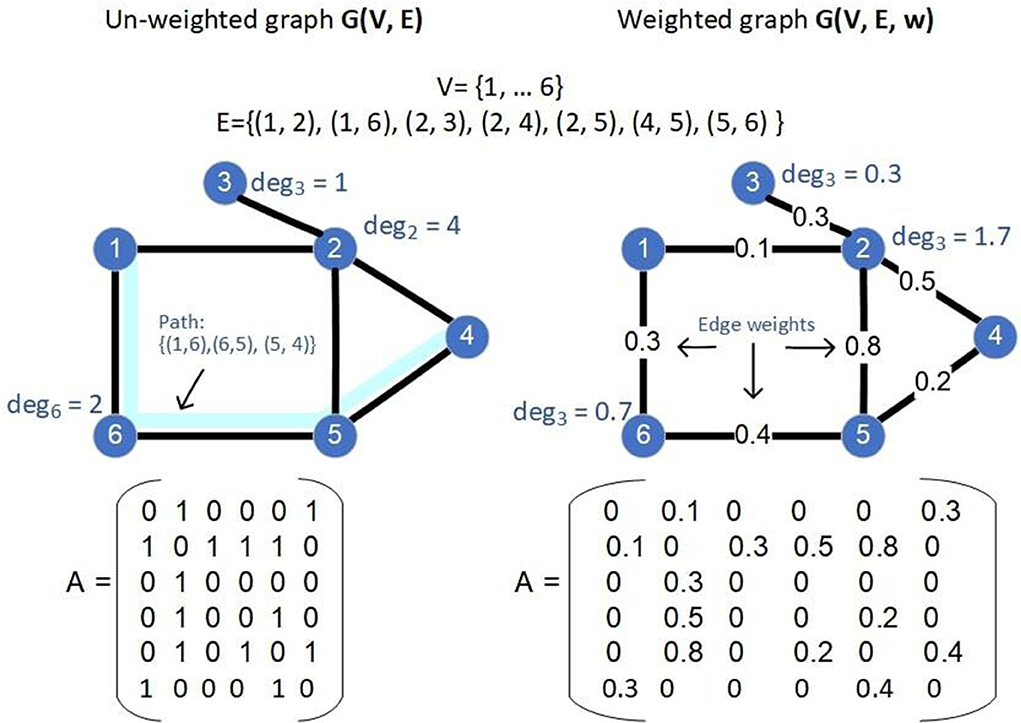
Figure 1. Two examples of graphs: an un-weighted one (left) and a weighted one (right), the values of the sets V, E and edge weights (in case of the weighted graph, specified by the function w), the adjacency matrix A, the degree of some nodes as well as a path (in light blue) are shown in the figure.

2.2.1.1. Similarity graphs

A similarity function associated with the edges of a graph is a function w:E → ℝ that measures how similar the corresponding nodes associated with each edge are. The corresponding graph and its adjacency matrix are called similarity graph and similarity matrix, respectively. Assume a set of N elements in a D−dimensional space, represented by ${\text{x}}_i\in {ℝ}^D$, for i = 1, …, N. A widely used non-linear similarity measure is the Gaussian kernel, defined in Section 2.1.2, where $w(i,j)\equiv exp(-\gamma ||{\text{x}}_i-{\text{x}}_j{||}^2),$ where ||x_i − x_j|| is the Euclidean distance between the vectors ${\text{x}}_i,{\text{x}}_j\in {ℝ}^D$ and γ = 1/2σ². There exist various suggestions for choosing the parameter σ, discussed in Sections 2.1.2 and in more detail in Section 2.1.3.

2.2.1.2. Graph sparsification

Graph sparsification is a graph simplification method that applies to the dense (complete) similarity graph in order to reduce its density, making the resulting graph sparse while keeping its most significant (of large relatively weights) edges. Two of the most common sparsification methods apply either a global or a local criterion for choosing which edges to be removed. Using a global threshold on the whole graph, we keep only the edges above that threshold [ϵ-neighborhood method [12]]. Using a local criterion, at each node, we keep the k largest weighted edges incident to it [k-nearest neighbor (k-nn) method⁹ [12]]. In order to choose the parameters ϵ, k there are no clear guidelines. However, we note that a basic prerequisite is that the resulting graph should be connected. In this work, we utilize the k-nn method for graph sparsification, with a careful choice for the value of k. In particular, we choose the parameter k using the mutual k-nn, in order to guarantee high levels of connectivity with mutually significant edges between nodes and then we apply the k-nn method for the construction of the sparsified graph, in order to guarantee connectivity between regions of different densities.

2.2.2. The graph clustering problem: Quality measures and algorithms

The graph clustering problem is the task of finding a partition ${C}$ of the nodes of the graph into groups, called clusters or communities, such that the nodes within each group are highly connected to each other, while the inter-crossing connections between nodes of different groups are as few as possible [20]. In this work, we consider similarity graphs. A clustering in such a graph reveals a partitioning into nodes of similar properties. Note that in graph clustering, the number of communities to be detected—denoted here by r—is not a priori known, in contrast to the similar problem of graph partitioning, where this information is part of the input of the problem¹⁰.

2.2.2.1. Quality measures of graph clustering

Modularity [21] is perhaps the most common measure of good graph clustering ${C}$, denoted by $m_{{C}}$. It measures the fraction of the edges that fall within clusters minus the expected number in an equivalent network where edges were distributed at random. Thus, the larger the value of the modularity is, the better the quality of the clustering. Note that $m_{{C}}\in \left[-1/2,1\right]$. The conductance of a cluster C [20] of a graph clustering ${C}$, denoted as h(C), is the fraction of edges with only one end in the cluster over the total number of edges of the cluster C (with either one of two ends in the cluster). The conductance of the clustering ${C}$ is the maximum such value over its clusters $C\in {C}$. Thus, the smaller the value of the conductance is, the better is the quality of the clustering. Note that $h_{{C}}\in \left[0,1\right]$.

2.2.2.2. Graph clustering algorithms

After the construction of the similarity graph and its sparsification, one can employ graph clustering algorithms in an attempt to simplify the system to significantly fewer entities—the clusters—which however manage to maintain the fundamental properties of the initial entities. This allows a characterization of the clusters of similar entities enabling finally the feature extraction of the initial complex system under investigation. Existing graph clustering algorithms follow several approaches for the detection of the clusters (or communities) in a given network, spanning from hierarchical ones [22] [agglomerative [23]] or divisive ones [e.g., [21, 24]], ones driven by various measures of clustering quality [e.g., modularity based [24, 25]], using various graph properties, such as edges or cycles [e.g., [26]], ones utilizing spectral graph theory [e.g., [27, 28]], and ones that combine the aforementioned approaches.

Here, we choose to present the results of two of the aforementioned approaches that follow a distinct method for obtaining the clusters: the first algorithm chosen is the Walktrap algorithm of Pons and Latapy [29] applied directly on the similarity graph, while the second one is a particular spectral graph clustering algorithm applied to the eigenvectors of the (Laplacian matrix) of the similarity graph to detect the clusters. The outputs of both algorithms are correspondingly evaluated using modularity and conductance as quality measures of the clustering obtained. The selected algorithms have been shown experimentally to obtain the most natural and representative results among several graph clustering algorithms tested.

The Walktrap algorithm is a hierarchical agglomerative algorithm. Using random walks to measure the similarity between two vertices, it detects network communities by building a hierarchy of clusters, starting from each node being a cluster of its own and merging pairs of clusters, trying to maximize the quality of the obtained clusters.

The second type of algorithm we utilize is the spectral graph clustering algorithm [12] and in particular the algorithm of Shi and Malik [28]¹¹. The algorithm uses the eigen decomposition of the un-normalized Laplacian matrix to perform a dimension reduction of the data space in a lower dimensional space, such that similar items are embedded closely in that space. It extracts the r (number of clusters to be detected) generalized eigenvectors of the un-normalized Laplacian of the graph, corresponding to the smallest eigenvalues. Finally, on this reduced dimension space, a standard clustering method then applies; typically the k-means clustering [30]. We note that this algorithm, as all other spectral clustering algorithms, requires the number of clusters r to be given as input. Here, for the specification of the value of r, we utilize a popular method followed, i.e., the eigengap heuristic [12].

2.3. A unified framework for feature extraction of complex systems

We now present a unified framework that brings together seemingly different approaches for modeling and analyzing complex systems, in particular principal component and graph theoretic analysis described above, under a common ground. This common ground allows one to understand better the differences, advantages, disadvantages, and commonalities between various approaches that can be used for analyzing a complex system, such as dimension reduction, clustering, and embeddings. Additionally, the framework does not provide a single procedure to follow but a number of computational paths or branches (i.e., PCA and Graph theoretical approach, and within each branch, other sub-branches). The framework is open to alternate usage of its elements. It can be used to analyze a complex system through a set of distinct questions. Each of these questions can be addressed by following different computational paths of the framework, as demonstrated in the Section 3.1.2. Different computational paths can be tested and compared for choosing the most suitable one to address each question. Finally, although it can be customized and enriched with domain knowledge, its individual steps are generic and domain independent. As a result, it is applicable to a wide range of scientific domains.

According to this framework, demonstrated in Figure 2, the analysis can be divided into the following steps and branches:

FIGURE 2

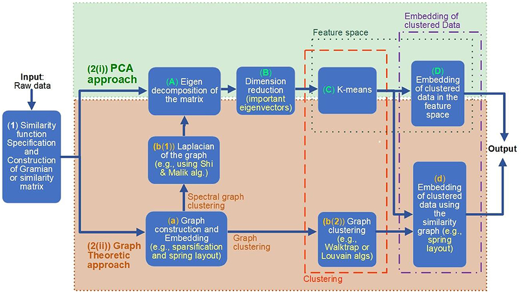
Figure 2. The unified framework for modeling, clustering, embedding, and feature extraction of complex systems. Various numbered boxes indicate the steps of the analysis. After the first step, where the appropriate similarity function is chosen and applied [box (1) of the figure], the framework allows two alternative computational paths to be followed; both of them allow a clustering (orange dotted surrounding box) and then embedding of the (clustered) data (purple dotted surrounding box): the principal component analysis (PCA) approach [indicated with green dotted surrounding box, numbered as 2(i)] or the graph theoretic approach [indicated with brown dotted surrounding box, numbered as 2(ii)]. Following the PCA approach computational path, the Gramian matrix is mapped to the Eigen space (i.e., the Feature space), where clustering is performed [boxes (A–C) of the figure]. On the other hand, following the graph theoretic computational path, the clustering is performed on the constructed similarity graph [computed in step (a)], either directly on the graph [box b(2)], following the graph clustering option (indicated with corresponding labeled arrow) or indirectly on the eigen space of the Laplacian of the graph, following box [b(2) and then (A–C)]. Finally, the clustered data are embedded either in the feature space [step (D)], if the PCA approach is followed, or through various graph embeddings (including also the eigen space embedding), in the case where the graph theoretic approach is chosen.

(1) The first step of the analysis [box (1) of Figure 2] takes as input the raw data of the problem (i.e., a collection of values (vectors or scalars) of the data set). During this step, a suitable Kernel function or the similarity function (see Sections 2.2.1.1 and 2.1.2) is specified. This function is then applied to the input raw data for the computation of the Gramian or similarity matrix.

(2) In the second step of the analysis, we distinguish two computational paths: (i) the PCA approach and (ii) the graph theoretic approach. Both approaches perform the tasks of clustering and embedding the data to reveal features of the complex system. The steps of each of these computational paths are indicated with colored dotted boxes surrounding them: a green surrounding box, numbered as [2(i)] PCA approach and a brown surrounding box, numbered as [2(ii)] Graph Theoretic approach, of Figure 2.

2(i) PCA approach

(A) Compute the N (N is the number of entities of the system) eigenvectors of the Gramian matrix G. Let V be the corresponding N × N matrix containing the eigenvectors of G as columns [box (A) of Figure 2].

(B) Select the first d columns of V. This reduced matrix gives the reduced feature space of data, capturing their d most significant features [box (B) of Figure 2]. For the specification of parameter d, the spectral gap method can be applied (refer to Sections 2.1 and 2.1.3).

(C) Now, in the reduced feature space of the data set, apply a data clustering algorithm, usually, the k-means [30] algorithm to cluster the data to groups of similar properties, according to the similarity function or Kernel chosen [box (C) of Figure 2]. For specification of the value of k needed for the k-means algorithm, again the spectral gap can be utilized as explained in Section 2.1.3.

(D) The final step of the analysis is to embed the clustered data in the feature space, selecting two or three of the principal components identified [box (D) of Figure 2]. This will reveal possible relations both between the clusters obtained but also with relation to other properties of the entities of the system.

2(ii)Graph Theoretic approach

(a) Alternatively, following a graph theoretic approach [surrounding dotted brown box 2(ii) of Figure 2], from the Gramian or similarity matrix computed in step (1), here we construct a sparsified version of the original dense graph (see Section 2.2), where the edges connecting pairs of entities with low similarity are removed. Finally, in this step, we display the constructed (sparse) graph using suitable embeddings, in order to visualize appropriate properties and relations between entities of the system under investigation. For example, we can use the force-directed layout [31], in order to place neighbor nodes closely in the plane. This step is shown in box (a) of Figure 2.

(b) The next step of the graph theoretic analysis is to apply graph clustering on the graph to obtain groups of entities (nodes in the graph) of similar properties [boxes b(1) and b(2) of Figure 2]. For this task, there are two alternative computational paths: either to move the graph in the eigenvectors space and perform the clustering in the reduced feature space or to apply graph clustering algorithms directly on the similarity graph. Each one of the two computation paths is indicated with corresponding labeled brown arrows in Figure 2.

- Spectral Graph clustering: Following this computational path, we basically apply the PCA method on the Laplacian of the graph, as described by some of the most popular spectral graph clustering algorithms, such as the Shi and Malik [28] algorithm: we first compute the Laplacian (or a variation of it) of the graph [step b(1)] and then (mainly) follow steps (A)–(C) of the PCA approach [surrounding box 2(i)] of the framework.

- Graph clustering: Following this computational path, we apply a graph clustering algorithm, such as the Louvain algorithm Blondel et al. [25], Leiden Traag et al. [32], or Pons and Latapy [29], directly to the (sparsified) similarity graph [box b(2)] of Figure 2).

(c) The final step of the graph theoretic approach is, similarly to the PCA approach, to draw or embed the graph with the clustered nodes (entities). The graph theoretic approach allows the embedding of the graph to be done either in the reduced feature space (eigenspace) selecting two or three of the principal components of the eigen decomposition of the graph [step (D) of the PCA approach] or using an appropriate graph layout, such as the force-directed layout [31], in which neighbor nodes are placed closely in the plane.

2.3.1. Discussion on the framework

As illustrated in Figure 2, the framework brings together different approaches for analyzing complex systems, i.e., a PCA approach [green surrounding box numbered as 2(i) PCA approach, of Figure 2] and a graph theoretic approach [brown surrounding box numbered as 2(ii) Graph Theoretic Approach, of Figure 2], under a common ground, in an aim to help analyzers to compare and choose between alternative computational paths as well to help for a better understanding of commonalities, differences, advantages, and disadvantages between the various computationally paths.

In particular, it distinguishes the different steps of the analysis, juxtaposing the characteristic of corresponding steps in each approach. For example, the representation of the system can be made through the eigen decomposition of the Gramian matrix, following the PCA approach [box (A) of the framework] or through the construction and corresponding embedding of the similarity graph, following the graph theoretic approach or through [box (a) of the framework]. The graph theoretic approach allows the visualization of the system data through the graph embedding while the eigen decomposition enables the representation of the data through another space, i.e., the feature space.

After the representation of the system, according to the framework, the next main step is clustering the data [surrounding orange box labeled as Clustering and boxes (C) and b(2) within it]. This task can be performed in the feature space, following the PCA approach [box (C)] or it can be performed either directly in the similarity graph [box b(2)] or indirectly on the reduced representation of the system through the most important eigenvectors of the Gramian matrix [box b(1)].

Finally, the last step of the framework is the embedding of the clustered data either of the reduced feature space or of the similarity graph (purple surrounding box, labeled as Embedding, of the framework). The PCA approach [green dotted surrounding box, numbered as 2(i)] allows the embedding to be done using combinations of the principal components (eigenvectors) of the reduced representation of the system. In contrast, the graph theoretic approach [green dotted surrounding box, numbered as 2(ii)] allows both an embedding using selections of the principal components (eigenvectors), through the spectral graph clustering computational branch of the graph theoretic approach, or using various graph embeddings, such as the spring-layout embedding that places neighbor nodes close in the plane.

Both the PCA and the graph theoretic approach possess individual characteristics, which can be seen as advantages or disadvantages by the analyzer, depending on the specific targeted goals of the analysis. Overall, the graph theoretic approach offers insights on the relations (similarities) between the entities of the system, through the various graph layouts, such as the force-directed layout [31]. However, these representations “loose” the real (initial) distances (dissimilarities) of the entities, and additionally most of the graph drawings use some randomization which makes the corresponding layout also non-deterministic.

2.4. Extensions of the framework

As already pointed out, the framework is flexible. It can be used for exploratory data analysis and to provide displays of skeleton results as part of an iterative procedure, as used in the first extension of the framework described next. It can also allow a mixed representation of what we might loosely refer to as structural and functional properties, as described in the second extension of the framework.

2.4.1. Labeling the terrain to make semantic maps

In the general framework we have outlined so far, results are represented in a way that is practically independent of the specific domain from where the data are coming from.

In the graph theory side of the representations, even the metric properties of the space are lost in the dimensionality reduction process. It is then difficult to assign a measure of how close the actual nodes which belong to a cluster are compared to nodes in other clusters. In the case of PCA, the metric properties are preserved and can be computed taking into account only the retained principal components. Nevertheless, there is no guarantee that nodes that appear close in the reduced space are not far apart in one or more of the hidden dimensions. If the reduced space is indeed representative of the natural patterns of interest in the data, large excursions in the hidden dimensions may represent noise or irrelevant information and hence the dimensionality reduction process can also be viewed as a noise elimination pre-processing.

In the non-linear kernel PCA, the same considerations hold regarding the metric properties within and beyond the retained spaces. In addition, the data are preferentially distributed in the native manifold described by the kernel function and the specific values chosen for its adjustable parameters. The images of the manifold (extracted from the data) can be useful tools. For example, consider two ways of introducing new data. First, new data can be generated by fresh measurements using the same sensors and processes as the ones used to record the original data. Second, new nodes can be generated by combining in some way a subset of nodes of the original data set, for example the nodes of predefined clusters. If the original data are dense and cover well the underlying manifold we would expect that newly introduced data will lie close to the original manifold, and can therefore be easily embedded in the existing displays. In the case of the generated data to represent clusters identified in the data set, the representative node representing each cluster can be defined by averaging the coordinates across the nodes of each cluster in each (reduced) dimension. All new nodes can then be added to the existing representation. In some applications, it is possible to make a preliminary assignment of each node on the basis of a priori information, accepting that some of the labels may be wrong. In such cases, for each cluster, a subset of the nodes within it can be used to define the representative nodes of that cluster. In this way, the original nodes can be hidden, maintaining in storage their coordinates and labels while leaving on the displays the representative nodes of each cluster and an image of the underlying manifold. The images of the cluster exemplars, which we will call CENTERS, can be displayed with the manifold derived from the original data. The process transforms the abstract mathematical distributions into a semantic map, i.e., a labeled map of the data terrain.

An iterative clustering approach can be defined to extract a skeleton of the underlying structure, derived directly from the input data. The linear PCA or the non-linear Gaussian Kernel PCA can first be used to define the reduced representation of the input data. A combination of prior information (if it is available) and clustering techniques can then be used to define distinct clusters. For each cluster, a representative prototype, the CENTER can be defined (if necessary excluding outliers). The display of the CENTERs in the reduced representation of the first few principal components constitutes an initial semantic map of the underlying structure. Each CENTER can in turn be expanded (bringing back outliers). The distribution of the nodes of the expanded center can be visually inspected to decide whether a single representative CENTER suffices or more than one CENTER must be defined, producing a sequence of refined semantic maps. Similar operations can be defined for merging nearby clusters (in the reduced representation), and the process is repeated to arrive at a more refined semantic map.

2.4.2. Transitions through geodesic paths

In many applications, the data separate into well-defined classes. The data between these classes define connecting pathways between the classes. Such pathways can be very important but, by nature, difficult to describe. The unified framework we propose offers a natural way of incorporating such pathways, as geodesic paths in the manifold defined by the combined data of the stable classes and the transition data. We simply embed the transition data into the existing manifold or recompute the manifold after augmenting the original data by adding the data belonging to transitions. In this way, the semantic maps of the last section become dynamic maps showing the transitions with the semantic maps in the background. This is particularly useful when different time scales are involved, which in the limit of very different dual time scales can describe structural/functional relationships. We will describe such an example in the first neuroscience application, where we show how the framework we propose can provide a powerful description of sleep with a semantic map providing the structural properties derived from periods of equilibrium (quiet periods of each sleep stage). Even during periods of apparently chaotic behavior, the dynamics can be described in a meaningful way. Nodes representing successive periods within a well-defined transition are connected in a strict chronological order and displayed as a path in the reduced space with labeled CENTERS serving as background (semantic map). A good example of such dual time-scale analysis is the first neuroscience application presented in Section 3.1.

3. Application of the unified framework in neuroscience and astrophysics

In this section, we demonstrate the application of the unified framework to three problems. The first two are from neuroscience, one dealing with a new approach to sleep staging and the other applying the framework for the clustering of early somatosensory evoked responses. The third one is from astrophysics and deals with the study of galaxy evolution.

3.1. Applications of the unified framework in neuroscience

3.1.1. Neuroscience background

Network analysis is highly relevant for modern neuroscience. Great advances in neuroimaging methods have demonstrated that brain function can be understood as a double parcellation of processing in space and time: “What appears as a noisy pattern when a single channel or a single area activation is observed from trial to trial, is seen to be less so when the activations between regions, across single trials, are examined” [33].

In the first parcellation, what we might call a structural network [34], the brain is partitioned into areas spread on the cortical mantle and in individual sub-cortical structures and their subdivisions. These areas are connected into well-defined networks. Some of these deal with processing signals from the sensory organs while others deal with attention, emotion arousal, and even the neural representation of self.

The second parcellation, what we might call a functional network [35], describes how particular processes evolve to accomplish specific tasks. Brain function involves an orchestrated organization in the time of cascades of activity within the nodes leading to diverging output from some nodes to many others and converging input on some nodes from many others. The normal operation of the functional network demands exquisite organization in time, which is achieved through multiplexing of interactions. We can think of them as cross-frequency coupling between the nodes of the network.

We distinguish two distinct ways of studying brain function and describe the application of our unified framework to one example from each one. In the first, we study periods of (apparent) quiescence which is further divided into resting states, awake state, and sleep stages; we show how the unified framework can guide the exploration of sleep stages and transitions between them. In the second, we study how the brain responds to well-defined stimulation; we show how the unified framework can help us separate responses to repeated identical median nerve stimulation into clusters. The input for this analysis will be special linear combinations of the raw magnetoencephalography (MEG) and electroencephalography (EEG) signals designed to selectively identify the first evoked responses at the level of the thalamus and cortex.

3.1.2. Classical and modern sleep staging

Sleep has been the subject of theorizing and speculation for millenia. The scientific study of sleep started in earnest in the early twentieth century with the pioneering studies of Dr. Nathaniel Kleitman in the first sleep laboratory established in the 1920s at the University of Chicago. Three decades of work culminated in the 1950s with landmark discoveries, including the identification of Rapid Eye Movement (REM) sleep [36]. The detailed study of sleep in many laboratories using the then available EEG technology led to the notion of distinctive periods of sleep, which was codified by Allan Rechtschaffen and Anthony Kales in the first guideline for assigning periods of sleep into “sleep stages” [37]. The guidelines depend on the identification of high amplitude or oscillations at specific frequencies that become the hallmarks of each sleep stage. The identification of these hallmarks assigns sleep period (usually 30 s) to undefined/movement, eyes closed waking before sleep (ECW), light or deep sleep, and REM. Non-REM (NREM) sleep is further divided into four parts, with NREM1 and NREM2 making up light sleep and NREM3 and NREM4 constituting deep sleep. Quiet periods with no graphoelements are found between periods with characteristic graphoelements of a given sleep stages; these quiet periods inherit the sleep stage label of such preceding periods, thus contributing to the smoothness of the sleep staging outcome. During each evening, a sleep cycle (SC), i.e., the progression from light to deep sleep and REM repeats three to five times. The resulting summary of a night's sleep is called hypnogram. The hypnogram has been the cornerstone for both sleep research and sleep medicine [35, 38].

A huge amount of research effort has been devoted to understanding the essence of each sleep stage through understanding its hallmarks, but with limited success. The key conclusion from this work has been the realization that each exemplar of a hallmark of a sleep stage was very different and that each one was made up of widely distributed and highly variable focal generators; in the case of spindles, the first and last focal generators were usually only detected better with MEG, with only a fraction of spindles extended widely in between and sometimes appeared as synchronous EEG events [39].

Classical sleep staging was introduced more than half a century ago, revolutionizing sleep research and clinical medicine. Nevertheless, at the time of its introduction, knowledge about brain processes and ways of monitoring them were limited compared to what is routinely available today. Using some of the new information that can be routinely extracted with today's EEG and MEG technology, it allows us to go beyond classical sleep staging and extend the description of sleep to periods where the standard hypnogram could not describe and even demonstrate that a different classification scheme may be more informative. For example, the sleep stage REM would separate into at least two clusters, as suggested recently [40]. Recent changes in sleep staging, collapse the two divisions of deep sleep into the new NREM3 sleep stage [41] and prescribe ways of resolving ambiguities when hallmarks of different sleep stages are identified within the same 30 s period used for sleep staging. In our recent work, we have ignored these recent changes because although they reinforce uniformity across sleep scoring by human experts, they have no other theoretical foundation and eliminate valuable details [42–45].

3.1.2.1. Problem specification

Classical sleep staging relies on human experts to interpret large excursions of the EEG recordings from the time domain descriptions. The implicit assumption that individual exemplars of each hallmark represented similar events is inconsistent with the Dehghani et al. [39] results and demonstrated to be wrong by more recent results using intracranial recordings [46–49] and tomography of MEG data [43, 45]. It, therefore, seems that the periods of large graphoelements are unlikely to be useful for revealing the key properties of each sleep stage because they are chaotic periods representing a system that has nearly gone out of control on its way back to equilibrium. A key result of our recent studies was the demonstration that the quiet periods of sleep that classical sleep staging ignores completely, far from being uninteresting and void of useful information, are in many respects the best representatives of the core characteristics of each sleep stage [50]. Our earlier results led us to the then disruptive claim that sleep staging is possible from the properties of core periods alone. We will provide evidence of the veracity of this claim in this subsection using the extensions of the framework we have described in Section 2.4. Since there is no time marker to time-lock events, this question is best addressed using spectral analysis as we will describe below. For this analysis, we used a unique set of whole night MEG data, collected from four subjects at the Brain Science Institute RIKEN, some 20 years ago [51]. We will show results from one subject which are typical of the results we obtained for each one of the four subjects.

3.1.2.2. Methodology utilized

The details of the analysis have been described elsewhere; magnetic field tomography (MFT) was used for extracting tomographic estimates of brain activity for each time slice of available MEG data [52, 53]. The full pipeline for preprocessing and MFT analysis leading to regional spectra of each 2 s segment of tomographic estimates of activity and further statistical analysis is described in detail [can be found in [43]]. For the purpose of the analysis in this subsection, 29 Regions of interest (ROI) are defined in areas of the brain known to change appreciably during sleep. The normalized regional spectral power, hereafter simply referred to as the regional spectra are then computed for each 2 s exemplar of MFT estimates of brain activity. We typically use 8 or more exemplars for each category of data (e.g., sleep stage). The regional spectra for each exemplar can be used over the entire spectrum 0–98 Hz in steps 0.2 Hz or reduced to the power within each of the classical bands, delta (1–4 Hz), theta (4–8 Hz), alpha (8–12 Hz), sigma (11–17 Hz), beta (15–35 Hz), low gamma (35–45 Hz), and high gamma (55–95 Hz).

The Gramian matrix [step (1) of the framework] is then constructed with each element computed as the Gaussian kernel of weighted overlaps of pairs of regional spectra. It is then used as the input for step (A) of the framework, for the computation of its eigen decomposition [step (B)], following the PCA approach [surrounding box 2(i)] of the framework. For the main clustering analysis [step (C) of the PCA approach of the framework], the input consists of three sets of data: the bulk of the data is from the noise data, ECW, and each sleep stage. The second set of events included in the analysis are from the hallmarks of NREM2, spindles, and unitary k-complexes (KC1) i.e., avoiding KCs running in succession. Finally, new nodes representing transitions or other periods (e.g, representing hallmarks of individual sleep stages) are added. For each hallmark exemplar, two regional spectra are used, one from the 2 s before the start of the hallmark and the other from the 2 s beginning with the stat of the hallmark. The final set consists of a set of three successive periods of the 2 s of undefined period between two sleep stages or between the awake state and sleep (i.e., transitions). The clustering is performed with ROI details presented at one of two resolutions. In the united ROI resolution, only the category of the time period is retained (e.g., sleep stage, transition etc.), while the identity of each ROI is lost. In the un-united resolution, each node represents the 2 s period for each ROI separately, i.e., a single united node splits into a number (in our case 29) of distinct nodes, one for each ROI. In general, PCA is sufficient for the analysis at the united resolution level, while for the un-united resolution, KPCA is more appropriate. We will show examples of both next.

An automatic approach to sleep staging is possible but tedious because the choice of frequencies and ROIs for best separation between pairs of sleep stages must be made and these can vary a little from subject to subject. Here, we followed a slightly different approach which is a natural progression from the classical procedures. The approach utilizes the Extension 2.4.1 of the framework. First, we used expert classification as a starting point. The centers for each sleep stage are then defined using all available exemplars, except extreme outliers. If transitions are included, then all exemplars of each transition are collapsed to their respective centers. At this point, the centers are defined by the list of indices of the chosen exemplars. The centers of each sleep stage are then embedded in the reduced space for the case of linear PCA or on the manifold in the case of the KPCA. The actual nodes are then hidden, leaving a skeleton display showing only the centers in the reduced dimensions or on the manifold.

A second iteration of the framework is then initiated validating the expert classification for each sleep stage in turn. The nodes of each category, one category each time, are expanded (made visible). Usually, either visual inspection of the distribution of nodes or a formal clustering approach is enough to make a confident decision whether the single center is maintained or more than one centers must be used to adequately describe poles with high node density. The outliers and the nodes of each new center are then hidden leaving at the end of the second iteration, a revised skeleton display of the new centers in the reduced space or on the manifold. Note that the centers representing transitions are not processed in the second iteration step. A final step can be added in which the outliers are returned to the display and any ones that now are close to one of the centers are incorporated in to it; this allows to completely reverse the original expert classification in a data driven way. The final presentation can represent the centers in either the reduced space on the manifold with any one or more categories expanded to show how the nodes representing individual exemplars are spread. Also, one or more of the centers representing transitions can be expanded and the nodes of each transition linked to a path by joining successive nodes for which an ordering is appropriate (for example close chronological order).

Finally, we showed the topology of categories (e.g., sleep stages) relative to each other and transitions between these categories in the labeled terrain, implementing extension 2.4.2 of the framework. The labeled terrain could be displayed across planes in the reduced dimensions of the linear space of the PCA components or as the manifold of the terrain formed by the KPCA analysis. Next, we presented four displays showing results for the analysis of the sleep of one subject; for the first two, we employed the linear PCA analysis, switching to its Gaussian Kernel extension for the last two displays.

3.1.2.3. Results

For the first analysis, we used eight exemplars of regional spectra for each set of the 29 ROIs of each sleep stage and the ECW condition. We also used the noise measurement of the MEG (recordings with the MEG system in exactly the same position as in the real MEG measurements, but with no subject in the shielded room). Exactly the same analysis is performed for the noise as for the real data to compute virtual brain activations in the time and frequency domain. The resulting virtual noise regional spectra are appended in the analysis as exemplars of an additional “noise” conditions, which we interpret as a generalized origin. The actual spread of the images of the noise exemplars represented the spread of this zero level activity. Finally, the analysis is performed for eight exemplars for the periods before and during the spindles and unitary k-complexes (KC1). We also add three 2 s periods corresponding to a quiet period just before the first NREM1 period, representing the transition from the awake state to light sleep. Counting all these cases, we have 91 nodes available for the united ROI resolution analysis and 2,639 nodes for the un-united ROI resolution.

In the first analysis, we use the united ROI resolution and perform a PCA analysis of the 91 nodes using as components all ROIs and all frequency steps. The procedure described in the previous section is used to define centers, one for each category, except for REM which we separate into two sub-categories. The results are displayed in Figure 3, which shows the clusters extracted by the analysis described above. This graph was generated by using the Euclidean distance on the feature space and an optimum threshold. The values above this threshold are given the value of zero. The non-zero elements of the resulting matrix were the edges of the graph with edge weight the inverse of each value (Euclidean distance). We also mark with separate colors the clusters extracted from the k-means algorithm [implementation of step (C) of the PCA approach 2(i) of the framework]. Using four clusters, the k-means algorithm groups the noise center and the noise nodes in a separate (black) cluster, the awake state, and transition into a second (red) cluster, both the two REM clusters and NREM1 into the third (deep blue) cluster and all remaining ones [NREM2, deep sleep, and the periods before and during the hallmarks of NREM2 (spindle and KC events)] into the fourth (pale blue cluster). The transition from awake state to light sleep is highlighted by connecting with heavy black, dash arrows the ECW center (C Sawake) to the sequence of transition nodes, finally connecting in a similar way the last of the transition nodes to the NREM1 center (C S1), providing a visualization of the path in the graph [implementation extension 2.4.2 of the PCA approach 2(i) of the framework].

FIGURE 3

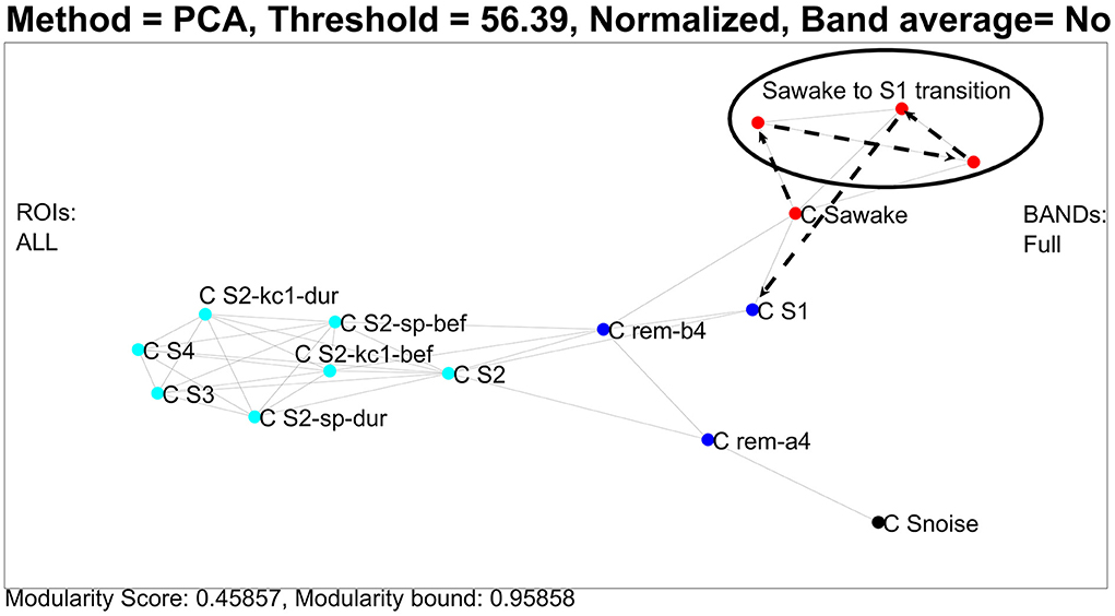
Figure 3. Clustering and transitions from eyes closed waking (ECW) to Non-REM1 (NREM1) on the semantic map defined by CENTERS of key sleep categories. To produce the figure, 94 (united) nodes were used, which were made up of the 91 nodes from core periods, awake, noise, and NREM2 hallmarks (pre and during spindles and KC1 events), and three nodes from the transition period from ECW to just before the NREM1 period. The details of the computations and what is actually displayed are described in the main text. The CENTER representations of the main categories are displayed in the reduced space of the first two eigenvectors of the PCA analysis providing a semantic map, on which the transition from ECW to sleep is portrayed by connecting (in chronological order) the nodes representing that period. For clarity and to avoid clutter in the display, the labels of the CENTER nodes begin with C and then S for the NREM sleep stage (e.g., C S1 for CENTER of NREM1) and obvious notations for the rest (e.g., C S2-sp- dur for the CENTER of the NREM2 period during spindles).

In the previous paragraph, the description of Figure 3 demonstrates how well the results of the united representation reflect the known properties of sleep stages, which in turn serve as a background for the dynamic display of the short transition from the awake state to sleep. The united approach collapses the details of regional spectra of each ROI for all exemplars of each category into one CENTER node. In the final representation, a single CENTER node represents the core period of each sleep stage or one of the other categories for which exemplars were included. This is a huge simplification, arrived through an essentially unsupervised application of the framework. The resulting display portrays well the known similarity between the classical sleep stages in a novel way. The skeleton of the representation is defined by the CENTERS of the core periods of each sleep stage. Within this skeleton the algorithm places in a very reasonable way two CENTERS for each hallmark of NREM2, one for the two second periods before and one for the two seconds that start with the onset of each hallmark event. Furthermore, a representation of a virtual baseline is included that provides a natural minimal level point of reference. The raw signal for this baseline are eight measurements, each of two second duration, recorded with no subject in the shielded room. These background noise measurements were processed in exactly the same way as the measurements with the subject in place. The regional spectra produced by these computation represented images of the background noise of the instrument and the ambient magnetic field inside the shielded room. The images of these eight noise exemplars were collapsed into a single CENTER, which is the best representation of the zero level of our data, which we refer to as a virtual origin for our skeleton representation. This static representation of the structure of sleep can serve as the background for the description of highly dynamic processes like transitions from the awake state to sleep and between sleep stages. The display thus summarizes an entire night's sleep of a single subject. A measure of what has been achieved can be appreciated by noting that, to the best of our knowledge, this is the first such representation of sleep, from either supervised or unsupervised analysis of sleep data. The result is also deceptively simple because underneath its simplicity lurks a more complex system, which can only be exposed if the un-united analysis is adopted, as we describe next. Figure 4 shows again the results of PCA analysis, but this time using the un-united ROI.

FIGURE 4

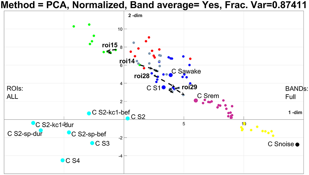
Figure 4. The results of PCA analysis using the un-united region of interest (ROI) resolution in the plane defined by the first two PCA. Exactly the same data are used as in the previous figure, and the same analysis, except that in collapsing the centers, each sleep stage, including REM, is represented by a single representative node (CENTER). The three nodes representing the transition from ECW to NREM1 in figure are now represented by 87 nodes and the single transition in Figure 3 is now represented by four paths, one for each V1 and FG in each hemisphere.

In Figure 4, each category of sleep is collapsed into one node (collapsing all exemplars and ROI nodes into one including REM), leaving only the nodes for each ROI for the three transition periods (3 × 29 = 87 nodes). Because of the large number of nodes, no attempt is made to produce a graph, thus no edges are shown in Figure 4. For this case, the nonlinear PCA is often a better representation (as we will explore in the next two figures), but for now, we stay with PCA, so there is a better correspondence in the methods when we compare Figures 3 and 4. Note that the k-means clustering (using seven clusters) maintains some of the patterns of the previous figure; the noise is still in a separate (black) cluster, and a separate (pale blue) cluster groups together NREM2 core periods and hallmarks with deep sleep (NREM3 and NREM4). This time ECW, NREM1, and REM are grouped into one (deep blue) cluster. Importantly, the transition period separates into a set of clusters beginning close to the noise cluster and extending across and beyond the REM (magenta), ECW and NREM1 (deep blue) cluster and beyond. The k-means cluster assigns some of the 87 nodes to the deep blue cluster and others to five more (yellow, magenta, gray, red, and green) clusters. These results suggest that collapsing all ROIs together may provide a powerful grand summary of sleep albeit, at the expense of missing considerable detail about the behavior of each ROI. An optimal description that may demand the use of more complicated methods may be appropriate, e.g., multilayer networks. Nevertheless, some useful observations can be made for the ROIs that are known to show distinct regional spectra for the start and end points of transitions. For example, in the classification of sleep stages from regional spectra, the ROIs for left and right primary visual cortex (V1) (14 and 15, respectively) and left and right Fusiform Gyrus (FG) (28 and 29, respectively) are effective for separating the awake state and NREM1. In Figure 4, the paths of the four regional spectra for V1 and FG are displayed (by connecting in the correct chronological order the three exemplars for the transition), showing that a consistent movement in the space of the two PCA, which is more apparent on the right hemisphere (ROIs 14 and 28). Finally, we draw attention to the pattern identified here for the transition from ECW to NREM1, more clearly seen in the united representation of Figure 3: the initial direction away from ECW is away from the NREM1 center, which just before the NREM1 onset, turns round 180° jumping to the NREM1 neighborhood of the semantic map. This pattern is not a peculiarity of this subject; it is identified in most other subjects during the first transition from ECW to NREM1 in SC1. This feature has important implications which are beyond this methodological paper and will be fully described elsewhere.

For the next two displays, Figures 5, 6, we use the same data in the un-united ROI resolution with the Gaussian kernel for the PCA analysis. We use only the noise, ECW, and the five sleep stages, which produce 1,624 nodes. The plot of the spectral gap shows two peaks, which correspond to two different scales in our data. The lower peak is found for γ = 0.003255 and corresponds to the scale appropriate for the variations encountered in the actual ROIs. The next display, Figure 5 shows the nodes spread in the ellipsoid with different colors representing the noise, ECW, and the different sleep stages, as these were defined by the human sleep experts. Note the importance of the noise data, which in the scale of the real brain activations are minute, thus collapsing to almost a point which we can use as the marker for the origin from which each node can be measured. There is a clear tendency for the nodes to spread in two dimensions with the long axis of the ellipse to describe a global increase, probably the overall strength of activations, while the variation in the orthogonal direction along the ellipsoid's surface to spread the nodes according to sleep stage membership. The pattern shows three bands. The lower band contains nodes belonging to awake (red), REM (yellow) and NREM1 (light green). The higher band contains nodes belonging to deep sleep, i.e. NREM3 and NREM4 shown by different pales of blue. Most NREM2 nodes (dark green) fall in the middle band on the ellipsoid surface, between the two bands described above.

FIGURE 5

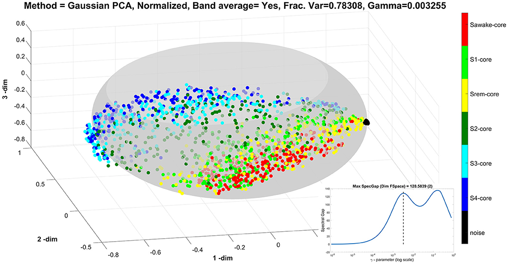
Figure 5. The results of Gaussian Kernel PCA analysis using the un-united ROI resolution in the 3D space defined by the first three PCA. There are over one and a half thousand nodes which are now labeled according to the category each one belongs (noise, ECW, and the five sleep stages). The insert shows the spectral gap as a function of the γ-parameter value in a semi-log scale, which has two peaks. The display shows the results using the value of γ at the first peak, marked by the dash vertical line in the insert (at γ = 0.00326). With this choice of γ, the nodes from the noise measurement collapse to almost a point which serves as the origin of the representation since it represents the region of feature space with very small values. The nodes corresponding to measurements with the subject in place are well-spread forming a good representation of the underlying ellipsoid.

FIGURE 6

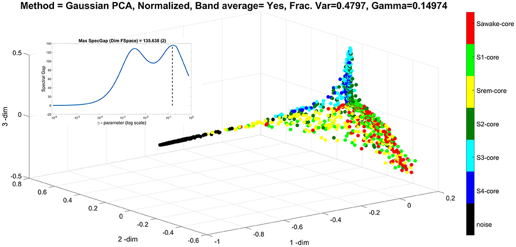
Figure 6. It is same as Figure 5, but for the value of γ at the second peak, marked by the dash vertical line in the insert (at γ = 0.1497). With this choice of γ, the ellipsoid is lost because the non-linear mapping emphasizes on the distribution of the nodes representing the low amplitude noise. In this case, the method selects the null (noise) direction of the data to be the first principal direction (the most important direction), while the remaining of the data are distributed along the second and third principal direction representing the amplitude of the deep and light sleep. The ellipsoid is lost because the non-linear representation emphasizes the representation of the nodes representing the low amplitude noise in the principal direction constraining the nodes representing the real data on the 2D plane of the second and third principal directions, thus projecting the ellipsoid onto a plane.

The final display for the sleep analysis, Figure 6 shows the same analysis as that of Figure 5, but with the γ = 0.1497, which is value of the second and higher peak (also marked here in the insert of the semi-log plot of spectral gap vs. the γ-value). This γ value is appropriate for the range of values of the virtual brain activations generated by the analysis of the noise data. These noise variations are very small compared to the real brain activations, except in the directions that are in the null (noise) space of the real data, where these are scaled to adequately represent their range (which actually is over a very small real magnitude). Therefore, the noise components in the directions where the real data are silent are emphasized, forcing the first principal direction along the null space of the real data. The real data are then branching off in two, nearly orthogonal, directions in the plane at right angles to the first principal direction defined by the noise measurements.

3.1.3. Clustering of single trials of early brain responses

3.1.3.1. Background

In the previous application, the brain was studied during sleep where no external stimuli is presented to the subject. In contrast, in this application, early brain responses elicited by stimulation of the median nerve of the wrist are analyzed. Such somatosensory stimulation gives rise to the so called somatosensory evoked potentials (SEP) and somatosensory evoked fields (SEF) that are recorded and seen in the EEG and MEG signals, respectively. These kind of brain responses are quite strong compared to the background activity of the brain, easily identified in the raw EEG/MEG signals, time-locked to the stimulus onset and one of the most reproducible brain responses to an external stimulus [54]. While this type of stimulation excites many areas across the brain, experiments with animals and humans have identified the times of the first arrival of the signal in the area of the thalamus [55–57] and in the cortical area S1 [55, 57–60].

Specifically, at around 14 ms after the presentation of the stimulus, a prominent positive peak is shown at the SEPs, called the P14 component; this is related to the neural activity in the thalamus [55, 56]. A few milliseconds later, around 20 ms post stimulus, peaks can be seen in both in SEPs and SEFs; this is related to the neural activity in S1 [55, 56, 60, 61]. The peaks at 20 ms, are known as P20 for EEG and M20 for MEG, and they are seen as dipolar patterns rotated by 90° to each other. Both the P20 and the M20 have been localized independently in the primary somatosensory cortex, Broadman area 3b [59, 60, 62]. For our purposes, the primary thing is that these are the first arrivals of the evoked response at the level of the thalamus and the cortex, and they are therefore the components that are least influenced by activity in the many other cortical areas that come later.

3.1.3.2. Problem specification

In experiments with EEG/MEG recordings in response to somatosensory stimulation, the stimulus is presented to the subject many times with a predefined interstimulus interval. Each repetition of the stimulus is called a trial. Even though responses to somatosensory stimulation are quite strong and time-locked to the stimulus, there are still some variations from trial to trial, for reasons that are not yet understood. Here, we explore the causes of these variations using the following two steps. First, the concept of the virtual sensor (VS) is used to get a good estimation of the underlying sources at the single trial level, then the framework is utilized for clustering of the single trial virtual sensor signals. The input to the unified framework for clustering is the time-domain signals extracted directly from the output of the VS applied to the raw signals.

3.1.3.3. Data and methods

The data used here are simultaneous EEG/MEG recordings from 1 human subject. The EEG/MEG recordings were made available to us in an anonymized form without any MR images, by the corresponding author of the study [60]. Experiment involved 1,198 trials (repetitions) of electrical stimulation of the median nerve at the right wrist of subject. The raw EEG and MEG data were cleaned from stimulation artifacts, line noise, and band pass filtered in the frequency range [20–250 Hz]. In the case of EEG, the mean of all channels was used for re-referencing the signals of the individual EEG electrodes. Once the data were cleaned and filtered, the continued data were epoched into trials of 0.3 s total duration. Each trial was defined as the signals starting 100 ms before (pre-stimulus period) and 200 ms after (post-stimulus period) stimulus onset. The next step was to group the trials into sets, such that the members of each set contained trials with the head in the same position relative to the MEG sensors. This was done by identifying the periods with head movement from visual inspection of the continuous MEG signals. Since the MEG sensors are stationary above the head, even slight movements of the head cause big distortions of the signals that can be easily distinguished visually. Finally, one group of 239 trials with no head movement was selected for further analysis. From the mean of the 239 trials, the P14 and M20 components were identified as prominent peaks at 14 and 20 ms after stimulus onset, respectively.

We know that even for the relatively strong stimulus used here, there is some variation in the responses of each trial. In order to get a good estimation of the time course of the underlying sources, one VS was defined for each component. Analysis of evoked responses using virtual sensors has been employed for the identification of early sensory responses for the somatosensory, auditory, and visual cortex [63–65]. A VS is constructed using a very simple procedure founded on well-understood physics principles for the generation of electric and magnetic fields. In this work, we construct two VS, the EEG P14-VS to get an estimate for the thalamic activity at around 14 ms, and the MEG M20-VS to get an estimate for the activity of S1 at 20 ms, using the EEG and MEG raw signals, respectively. Here, the selection of the channels for the construction of the two VS is based on the signal power (SP) and signal to noise ratio (SNR) at the specific latencies (14, 20 ms) and across all the 239 trials. The definition of the VS is fixed from the average signal at the time points of little variation of the first thalamic and primary somatosensory cortex (BA 3b) from the average of the ensemble of all trials. The estimate of each thalamic and cortical (BA 3b) response is then estimated from the signals of each individual trial.

For the strong median nerve stimulation used in this experiment, the evoked response at the level of the cortex is present in almost all single trials. The M20 corresponds to the first arrival at the cortex and there is little interference from any other generators since all previous responses were at the level of the thalamus and the brainstem. We can therefore assume that the M20-VS estimates within the first 20 ms correspond to the activity of the primary somatosensory cortex. In contrast, the thalamic activity around 14 ms is likely to have some contribution from other deeper brain activations corresponding to the arrival of the slower components of the evoked responses or even different pathways. Hence, the EEG P14-VS estimates at the ST level will vary. We use the unified framework to cluster the 239 trials into groups of trials. The clustering is applied to the signals from both VS, separately.

First, we use the Gaussian Kernel as a similarity function on the trial signals, to construct a similarity matrix [step (1) of the framework, see Figure 2]. In the resulting graph, the nodes represent the single trials and the edges between nodes measure how similar the corresponding nodes (trials) are. Next, we apply graph sparsification [step (a) of the graph theoretic approach 2(ii) of the framework] in order to get a good visualization of the corresponding similarity graph. Then, we utilize the spectral graph clustering computational path, following steps [b(1)] and (A)–(C) of the framework, to detect nodes (trials) with similar signals. The last step of the graph theoretic analysis is to draw the graph, using the force-directed layout [31] and show the detected clusters [step (d) of the framework]. Once the single trials (nodes) have been assigned to different clusters, we compute and show the average signal for each detected cluster.

Finally, functional connectivity [3] analysis on a single trial level is performed between the clusters of the two different VS. This is done with the goal to identify possible communication mechanisms between the two areas (thalamus—cortex) in response to somatosensory stimulation. The Pearson's correlation coefficient (PCC) in a fixed window of 8 ms length and with introduced time delays at every 0.833 ms, is used to quantify the values of the time-delayed correlation between the time courses of two signals.

For the implementation part, we have developed our own Matlab code for extracting and pre-processing the necessary data from this data set and for the connectivity analysis. Also, we have employed Python and the package igraph for the graph theoretical analysis employed.

3.1.3.4. Results

Figure 7 shows the results of the graph clustering of the VS single trial signals for case of the P14-VS (left plot) and M20-VS (right plot). For the embedding of (clustered) data, the step (d) of the approach [2(ii)] of the framework has been used. In order to explore the differences between the signals belonging to each cluster, we compute and plot the average time-course across the signals (nodes) of the same cluster. The results are shown in Figure 8. As expected, in the case of the M20-VS signals (Figure 7B), there are fewer clusters (three clusters) compared to the P14-VS signals (five clusters). More importantly, all three clusters extracted from the M20-VS show the first peak at exactly the same latency, 20 ms. In contrast, the five clusters extracted from the P14-VS show distinct peaks for a range of latencies before and after the expected peak at 14 ms. This is an argument that the “thalamic” VS picks up strong contributions from more than one deep area.

FIGURE 7

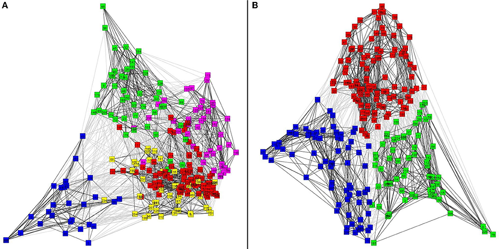
Figure 7. The clusters of virtual sensors (VS) single trial signals obtained. (A) Shows with different colors, five clusters for the P14-VS detected using the Shi and Malik [28] algorithm and obtained modularity = 0.36 and conductance = 0.44. (B) Shows three clusters for the M20-VS, detected using the Shi and Malik [28] algorithm and obtained modularity = 0.45 and conductance = 0.27.

FIGURE 8

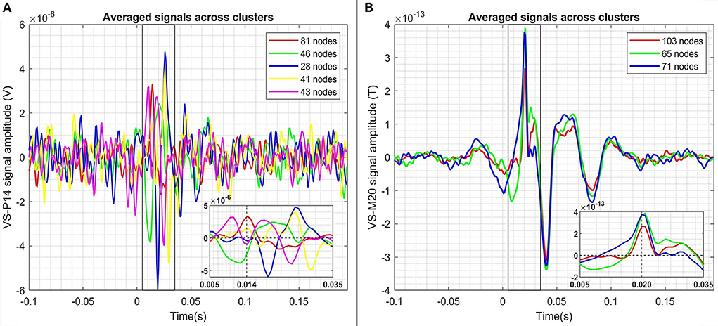
Figure 8. The mean of the signals belonging to each of the clusters of the two different virtual sensor's data. (A,B) Show the mean of the trials in each cluster for the P14-Vs (thalamus) and the M20-VS, respectively. On the right bottom of each plot, a zoomed version of the cluster averages is displayed in the time window from 10 to 40 ms post-stimulus.

The cluster with 81 nodes in P14-VS clusters (red color in Figure 8A) shows a prominent and distinct peak at 14 ms.There are two main reasons that allow us to relate this peak at 14 ms with the activation in the thalamus. First, the spatial filter applied by the P14-VS captures the electric field at the surface of the head that is generated by a radially oriented source in the brain, as a source in the thalamus is expected to be oriented. Second, other studies have reported that this peak at 14 ms is generated by neuronal activity in the ventral posterolateral nucleus (VPL) of the thalamus in response to median nerve stimulation [55, 56].

The functional connectivity between the thalamus (P14-VS) and the cortex (M20-VS) was estimated for the trials in cluster 1 (81 trials) of the P14-VS. For each trial, the time-delayed correlation coefficient (CC) was calculated with a moving window of 8 ms. The correlation values are shown in Figure 9. The left plot shows the correlation values at all time points and all the time-delays used, while the right plot is a zoomed version to show the exact timings of the significant CC values. The red contour lines show the areas (times and time delays) with statistically significant correlation values (p < 0.05, Bonferroni Correction). As can be seen in the zoom in version of the results (right plot Figure 9), at around 14 ms (x-axis), the signal of P14-VS is highly correlated with the signal of M20-VS with two different time delays, 5.8 and 18.3 ms (y-axis).

FIGURE 9

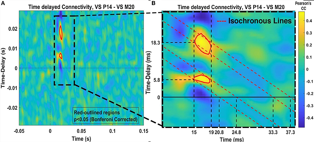
Figure 9. Single trial functional connectivity results between VS signals P14-VS and M20-VS, for the trials belonging to Cluster 1 (81 trials) of the P14-VS (see Figure 7A). (A) Shows a color map with the correlation coefficient values at each time and time-delay. The red outlined areas show statistically significant values (p < 0.05, Bonferroni correction). (B) Shows a zoom-in version of the figure in (A), which shows in more detail the precise timing of start and end times of the statistically significant increases in connectivity values.

The results suggest that there are two waves both starting at the same latency from the thalamus and arriving at the cortex with different time-delays. The first wave starts at 14 ms and reaches the cortex at 5.8 ms later (20.8 ms), and the second wave arrives at the cortex 18.3 ms later (33.3 ms). It is worth mentioning that both waves last ~4 ms. The first wave arriving at the cortex begins at 20.8 ms and ends at 24.8 ms while the second wave begins at 33.3 ms and ends at 37.3 ms. In both waves, the CC values suggest that there might be a continuous traveling of information (communication) from the thalamus to the cortex that lasts around 4 ms.

The different time delays of the two waves (5.8 and 18.3 ms) might be due to the conduction of the electrical signals through two distinct neural pathways. One possible explanation is that the first pathway might consist of heavily myelinated fibers with high conductivity and speed, while the second pathway is through less myelinated fibers of lower conductivity slower by a factor of three relative to the first one. This ratio between the conductivity speed of the two fiber types is reflected to the different time delays of 5.8 and 18.3 ms. This explanation invites further investigation using other functional connectivity measures and data from more subjects.

To summarize the outcome of this subsection, the use of the unified framework for performing clustering on the VS Signals extracted from the simultaneous EEG-MEG recordings allowed us to identify and assess thalamocortical functional connectivity only by using directly the pre - processed EEG/MEG data (e.g., without utilizing any source reconstruction algorithms). Our functional connectivity results show that there is information flow between the thalamus and the cortex in response to median nerve stimulation, which is consistent with results of other studies [55, 66, 67].

3.2. Astrophysics

3.2.1. Astrophysical background

A major field of study and open question in astrophysical research is the study of galaxy formation and evolution. In this study, we specifically focus on the evolution of ultraluminous infrared galaxies (ULIRGs): pairs of galaxies that are interacting gravitationally. During this interaction, the galaxies collide and ultimately merge into a larger—usually elliptical—galaxy. This process (which is called a “merger” event) results in an increase in luminosity, mainly in the infrared part of the spectrum. This luminosity increase is primarily caused by the burst of star formation activity inside these galaxies and/or the accretion of matter onto the galaxies' supermassive black hole (SMBH). Galaxies that display a high star formation rate are called “starburst galaxies.” Recent models of galactic mergers have shown that galaxies in the post-merger phase display an increase in activity in their core, where the SMBH resides. An active SMBH at the center of a galaxy is called an active galactic nucleus (or AGN). Starburst galaxies display different characteristics than galaxies that go through an AGN-dominated phase. During the starburst phase, the galaxy contains large quantities of gas and dust, which collapse under gravity to form new stars at a very high rate. During the AGN-dominated phase, large amounts of gas are accreted onto the SMBH and are subsequently ejected from the galaxy via highly energetic outflows and jets. The effects of these processes result in certain differences in the observed characteristics in the spectra of ULIRGs and studying these differences is the key to understanding the evolutionary stages these galaxies go through.

3.2.2. Problem specification

In order to understand the numerous processes that govern galaxy formation and evolution (quiescent star formation, bursts of star formation, and accretion onto SMBHs), multi-wavelength or panchromatic observations of galaxies at all cosmic epochs are needed. The necessity to characterize the panchromatic emission of galaxies has led to a series of surveys at all wavelengths, from X-rays to radio emission, with ever improving sensitivity, resolution, and sky coverage. Most of the surveys can only be carried out from space, so this became possible mainly in the last two or three decades with missions such as IRAS, ISO, Spitzer, AKARI, Herschel, Planck, WISE, and GALEX. One of the most important conclusions arising from the study of the panchromatic spectral energy distributions (SEDs) of galaxies in recent years is that the properties of luminous galaxies at high redshift are distinctly different from those at low redshift. The most luminous infrared galaxies at low redshift are associated with mergers but this does not appear to be the norm in the distant universe [e.g., [68]]. Establishing the fraction of luminous infrared galaxies at high redshift that are caused by mergers is a subject of current research. Recent research [e.g., [69]] also suggests that even if mergers were present in the early Universe, they were probably not as efficient at causing starburst events as in the local Universe.

The inference from the SEDs of galaxies to determine their nature traditionally involves taking into account a range of processes. These include stellar population synthesis models [e.g., [70, 71]] and models describing how the presence of cosmic dust in the interstellar medium of galaxies affects significantly their ultraviolet (UV) to millimeter spectra (which covers the wavelength range from 0.1 to 1,000 μm). Models for the latter treat the effects of dust either in a simplified geometry (e.g., in codes like MAGPHYS and CIGALE) or in more detailed treatments like radiative transfer models [e.g., GRASIL by [72–75]].

In the present work, we study the evolution of ULIRGs by employing the graph theoretic approach of the unified framework [2(ii)], described in detail in the following sections. The results we present here are part of the more extensive work of Pavlou et al. [76].

3.2.2.1. Data description

To study ULIRGs, we gather and analyze data collected by the infrared spectrograph (IRS) onboard NASA's Spitzer Space Telescope. We study publicly available low and high-resolution IRS data provided by the “Combined Atlas of Sources with Spitzer IRS Spectra” (CASSIS) website at https://cassis.sirtf.com/. These data are provided in the form of tables and graphs of spectral flux density (F_ν) over wavelength (λ).

3.2.3. Methodology utilized

We investigate data for galaxies taken at mid-infrared wavelengths, combined with other physical properties of the galaxies, employing the unified framework and following the graph theoretic approach.

Initially, we employ the Gaussian Kernel as a similarity function on the galaxies SEDs to construct a similarity matrix [step (1) of the framework]. Then, following the graph theoretic approach [surrounding box 2(ii) of the framework], we construct the corresponding similarity graph, where ULIRGs are represented as the nodes of the graph and edges between nodes are constructed as a measure of the similarity between the SEDs of the corresponding nodes (galaxies). The resulting graph is obtained by applying a graph sparsification in the similarity matrix [step (a) of the Graph Theoretic approach]. Then, we explore various graph clustering algorithms [both steps b(1) or b(2)] for detecting nodes of similar SEDs, corresponding to galaxies of similar evolutionary stages, in order to extract an evolutionary paradigm for ULIRGs.

The last step of the graph theoretic analysis is to employ suitable graph embeddings [step (c) of the graph theoretic approach], such as the force-directed layout [31], to show and compare the detected SED clusters with other physical properties of the galaxies, such as the 6.2μm polycyclic aromatic hydrocarbon (PAH) emission and the silicate absorption/emission feature, using the graph drawing. Furthermore, we compute and present the average SEDs of each detected cluster.

Finally, we perform an interpretation of the graph theoretical outputs, employing domain specific knowledge. The outcome of this analysis based on graph theory produces a description of the evolution of ULIRGs from the pre-merger phase up to their AGN-dominated and/or quasi-stellar object (QSO) phases. This offers a data driven alternative to the (domain oriented) “Fork diagram,” introduced by [77].

For the implementation part, we have developed our own Python code for extracting and pre-processing the necessary data from this data set. Also, we have employed Python and the package igraph for the graph theoretical analysis employed.

3.2.4. Related work

Despite the long history of graph theory and its successful application in various sciences, there are very few works that exploit graph theory in order to study problems in Astrophysics. A prominent work is the paper of Farrah et al. [18]. This work's methodology represents the main research motivation for our own astrophysics research project. The authors of this paper studied a sample of local ULIRGs (z < 0.4) with low-resolution data from the Spitzer/IRS instrument by combining the methods of graph theory and Bayesian inferencing, in an attempt to identify and distinguish between different phases of temporal evolution.

The study of specific galactic features, such as the correlation between the PAH emission and star formation in galaxies, enables the distinction between different evolutionary stages. The relationship between PAH emission and star formation in nearby galaxies at z < 0.2 was also examined by Murata et al. [78]. Analysis of data obtained by several instruments (namely AKARI, WISE, IRAS, Hubble Space Telescope, and SDSS), led to an investigation of 55 star-forming galaxies and the discovery that PAH emissions are partially extinguished during the later stages of galactic mergers. The authors determined that the main causes for this extinction are strong radiation fields and large-scale shocks taking place during the merger events. Shipley et al. [79] studied the PAH emission features in high-redshift galaxies (1<z<3) in order to calibrate their star formation rates (SFRs). Using Spitzer (IRS) observations, they demonstrated how PAH emissions can accurately describe SFRs in galaxies and thus help distinguish between star-forming and AGN-dominated galaxies.

A classification of the evolutionary phase of galaxies via the study of silicate absorption/emission strength and PAH emissions in the mid-IR range were also performed by Spoon et al. [77]. The authors showcased how specific emission features, such as PAHs at 6.2μm and silicate absorption at 9.7μm can betused as indicators to distinguish between starburst and AGN-dominated galaxies. Their results are presented graphically, in the form of a “Fork” classification diagram.

Although the exploration of graph theory in astrophysics is limited, a more extensive research literature is available in the field of cosmology, with very interesting results. In particular, Coutinho et al. [80] utilized dynamical network analysis to cosmological models of large-scale structure, containing a simulated number of galaxy distributions, in order to study the gravitational interactions and evolution of galaxy clusters and superclusters. Additionally, Hong and Dey [81] as well as Sabiu et al. [82] demonstrated how graph theoretical methods and tools can be successfully applied on simulated and observational data. All of the aforementioned works suggest that, by extension, the application of graph theory can also be a very useful tool in cosmological studies of galaxy formation and distribution.

3.2.5. Results

In this section, we present the results we obtain by applying the unified framework for the astrophysics problem described above.

3.2.5.1. The similarity graph

We first use the raw data (SEDs) of 139 galaxies (102 ULIRGs and 37 quasars) to construct the similarity matrix, using the Gaussian Kernel (see Section 2.1.2), implementing step (1) of the framework. For choosing the value of σ, we use the SD of the sample (see Section 2.2.2.2) obtaining a value of σ = 0.0328.

In this application of the unified framework, we follow the graph theoretic approach [surrounding box 2(ii)]. Thus, we next apply a sparsification of the similarity matrix to obtain the similarity graph [step (a)]. We are interested in maintaining both connectedness (i.e., the graph to be connected) and an adequate representation of the original data. Applying the k-nn method, the connectedness requirement is achieved with very small values of k, which leads to a very sparse graph. Thus, we use the mutual k-nn (where connectedness is achieved for higher values of k). We choose the smallest k for which the size of the largest connected component is stabilized. Having chosen an appropriate parameter k and given that connectedness is not guaranteed in mutual k-nn, we apply the selected value of k in the ordinary k-nn method (since the mutual k-nn method results in a subgraph of the graph resulting from the k-nn method).

Applying this heuristic we obtain that k = 6. A drawing of the resulting sparsified graph (in a two-dimensional space) is shown in Figure 10. For the drawing, we use the force-directed layout algorithm of Jacomy et al. [31]. Force-directed layout algorithms [83] produce graph drawings (layouts) of as few crossing edges as possible (by assigning forces between nodes so that neighboring nodes are placed closely in the plane).

FIGURE 10

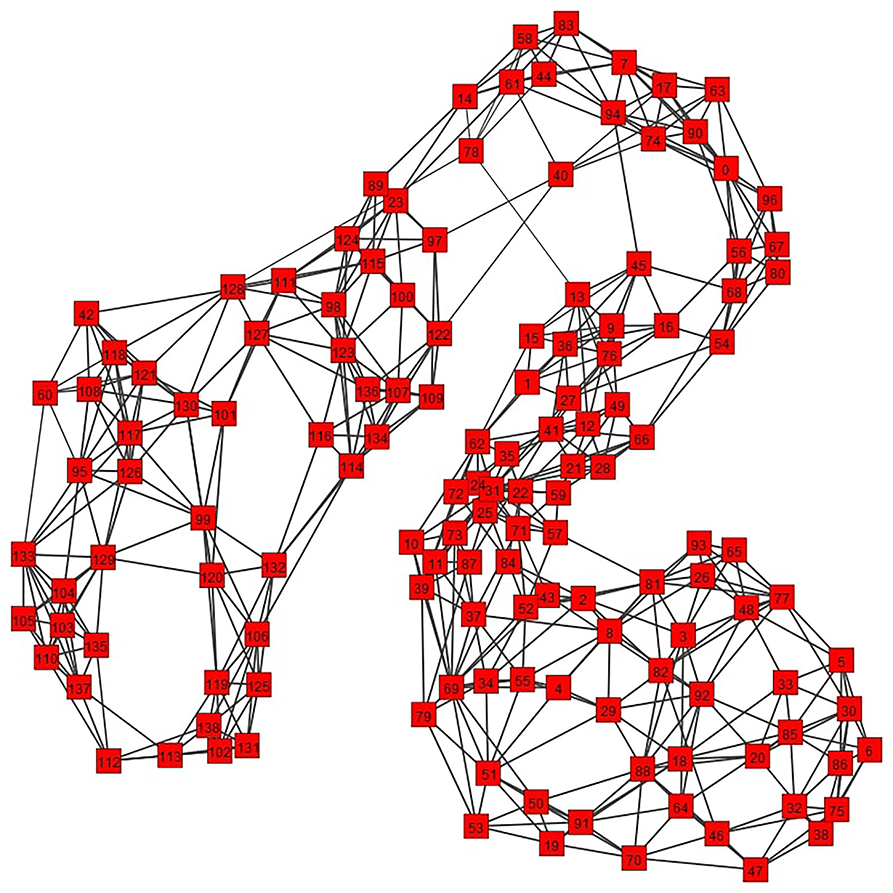
Figure 10. A force-directed layout [31] of the resulting (sparsified) similarity graph, which uses the Gaussian Kernel as a similarity function.

3.2.5.2. Extraction of SED communities

Next, we apply graph clustering algorithms on the SED similarity graph, to detect galaxies of similar SEDs [steps b(1) and b(2) of the framework]. We have tested several graph clustering algorithms (described in Section 2.2.2.2), obtaining similar results. This similarity in the detected clusters from different clustering algorithms is an indication on the robustness of the results of this methodology. Here, we present the most representative results, obtained by the implementation of the Walktrap algorithm [29], which applies directly to the adjacency matrix of the similarity graph [step b(2) of the framework], and the spectral graph clustering algorithm of Shi and Malik [28], which applies to the eigenvalues of the Laplacian of the similarity graph (more details are provided in Section 2.2.2), following steps b(1) and (A)–(C) of the framework. For the specification of the number of clusters to be detected, which is required by both algorithms, applying the method described in Section 2.2.2, we select the number of clusters that maximizes the quality of the clustering obtained both in terms of modularity and conductance. By using this quantitative criterion, both algorithms detect five clusters as the optimal number.

Figure 11 shows the clusters identified by these two graph clustering algorithms [(a) Shi and Malik algorithm and (b) Walktrap algorithm], using the force-directed layout of Jacomy et al. [31] [step (c) of the framework]. Interestingly, both algorithms achieve the same modularity score (0.7) and conductance value (0.111) of the clustering obtained.

FIGURE 11

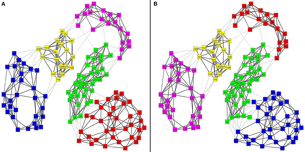
Figure 11. Five clusters identified from the Shi and Malik algorithm (A) (modularity = 0.70 and conductance = 0.11) and Walktrap algorithm (B) (modularity = 0.70 and conductance = 0.11).

3.2.5.3. Interpretation of communities detected, relations with other physical properties, discussion, and comparison

The outcome of the application of the unified framework is now utilized for the interpretation of the results obtained. A first interesting observation of the clustering obtained (Figure 11A) is that the clusters form a (higher level) path graph: that is, the vertices of the blue cluster are connected to the vertices of the yellow cluster, which is connected to the purple one, which is, in turn, connected to the green one, which finally is connected to the red cluster. This path formed between clusters may suggest a quasilinear evolutionary path for these galaxies. Let us call this path as the path of clusters of galaxies.

First, in order to characterize the clusters detected, we compute the average SEDs of galaxies in each detected cluster. The result is shown in Figure 12. We observe that the graph clusterings manage to distinguish between galaxies of seemingly different SEDs. Furthermore, we observe that there is a consistency between “neighboring” average SEDs in Figure 12 and neighboring clusters in the path of clusters of galaxies formed by the clustering. PAH emission and silicate absorption features are clearly observable in the red and green clusters, indicators of intense star-forming (starburst) activity present in these galaxies. Conversely, these features are mostly extinguished in the yellow and blue clusters, which are consistent with AGN-dominant activity taking place in the galaxies of these clusters.

FIGURE 12

Figure 12. The average spectral energy distributions (SEDs) of galaxies in each one of the detected clusters [as obtained by the Shi and Malik [28] algorithm]. Note that each average SED is colored with the same color as the corresponding cluster obtained by the Shi and Malik algorithm.

An interesting question is whether the communities detected using the galaxies' SEDs are related to other physical properties of the galaxies, and in particular, the PAH emission features of the galaxies as well as their silicate absorption/emission feature. We utilize graph theory to address this question. We apply a color mapping on the nodes of the graph using their value in the particular property under investigation. Figure 13 shows the color mapping of the nodes using the 9.7μm silicate absorption/emission feature distribution on the graph. The transition from weak to strong silicate emission between AGN-dominated PG quasars (blue–yellow clusters) and starburst galaxies (green–red clusters) is clearly distinguishable. A corresponding color mapping of the graph for the 6.2 μm PAH feature is shown in the Appendix.

FIGURE 13

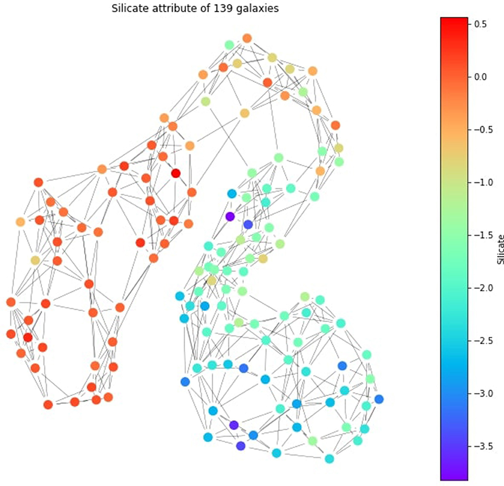
Figure 13. The Silicate absorption/emission feature distribution on the graph. The transition from weak to strong silicate between PG quasars (orange-cyan clusters) and starburst galaxies (green-yellow clusters) is clearly observable.

We note that it is very interesting that while our classification utilizes a different approach than the well established Spoon classification fork diagram [77], it is quite consistent to it. Additionally, it provides an alternative embedding of the galaxies through the graph drawing (compared to the PAH-Silicate plane utilized in Spoon et al.). These results are consistent with the current theoretical framework for the evolution of ULIRGs, based on the merger scenario, with ULIRGs displaying characteristics of starburst galaxies in the pre-merger stage (red-green clusters) and AGN-dominated quasar properties in the post-merger stage (yellow-blue clusters). Thus, the implementation of graph theoretical tools and clustering analysis on galaxy data can successfully identify and distinguish between different evolutionary stages of galaxy mergers. Finally, the application of the unified framework (following the graph theoretic approach) extends the grouping of Farrah et al. [18], which is based on the graph layout the authors obtained.

4. General discussion and conclusions

In this article, we presented a framework for the analysis of complex systems, which brings together classical and modern techniques from graph theory and PCA. The framework provides a network modeling of the complex data and provides a mapping of the multidimensional, complex data into lower dimensional spaces and embeddings. It allows first a clustering of the data into groups of similar entities and then through appropriate embeddings (representations) the extraction of the most important properties characterizing the system, i.e., extracting the most important feature of the complex system. The framework was demonstrated in three applications: one originating in astrophysics and two from neuroscience. The power of the framework lies in the flexibility it offers: it is based on sound mathematical foundations that can be applied to diverse domains knowledge, providing a useful tool for exploring and visualizing data from a wide range of sciences.

Author contributions

AI and VP contributed in Sections 1, 2, 3, and 4. CKo contributed in sections 3.1 and 3.2. CKa and LL contributed in Section 3.1. IM contributed in Sections 2.2, 2.3, and 3.2. MP contributed in Sections 2.2, 3.1, and 3.2. OP contributed in Sections 2.2 and 3.2. EP contributed in Sections 1, 2.1, and 3.1. AE contributed in sections 3 and 4. All authors contributed to the article and approved the submitted version.

Funding

The main work leading to the unified framework described here was performed under the project EXCELLENCE/1216/0207/GRATOS funded by the Cyprus Research & Innovation Foundation. Parts of the sleep staging neuroscience application were performed under the European Space Agency (ESA) Contract NEA2RS No. 4000127142. CKa and MP are early-stage researchers under the I-CONN project, which has received funding from the European Union's Horizon 2020 research and innovation program under the Marie Sklodowaka-Curie grant agreement No. 859937.

Conflict of interest

Authors AI, CKo, and LL are employed by the company AAI Scientific Cultural Services Ltd (AAISCS). Author CKa is an early stage researcher placed at AAISCS and doing his PhD at AAISCS within the I-CONN project consortium which has received funding from the European Union's Horizon2020 under the Marie Sklodowaka-Curie grant agreement No. 859937. The work at AAISCS places no commercial or financial constraints on any of the authors related to the work reported in this article.

The remaining authors declare that the research was conducted in the absence of any commercial or financial relationships that could be construed as a potential conflict of interest.

Publisher's note

All claims expressed in this article are solely those of the authors and do not necessarily represent those of their affiliated organizations, or those of the publisher, the editors and the reviewers. Any product that may be evaluated in this article, or claim that may be made by its manufacturer, is not guaranteed or endorsed by the publisher.

Footnotes

1. ^[N] = {1, 2, …, N}.

2. ^$\mu =\frac{1}{N}{\text{Σ}}_{i=1}^N{\text{x}}_i\in {ℝ}^D$.

3. ^Optimality here means maximization of the projected variance of the data [for more details, see [5, 6]].

4. ^The total variance of the data is then given by the sum of the eigenvalues $var(D)={\text{Σ}}_{j=1}^D{\text{λ}}_i$.

5. ^Due to the fact that the non-zero eigenvalues of the matrix $\tilde{\text{S}}$ are identical with the eigenvalues of its transpose [[10], p. 555].

6. ^according to ${\parallel {\text{w}}_i\parallel }^2={{\widetilde{\text{λ}}}_i}^{-1}$.

7. ^A function which can be viewed as a matrix with positive eigenvalues.

8. ^The D degree matrix of G is the diagonal matrix (having non-zero values only in its diagonal) for which the value of the entry i is the degree of vertex i of G.

9. ^The parameter k used in the k-nn should not be confused with the k used in the k-means algorithm, also discussed in this paper; we use the same letter (k) in both algorithms, since it is actually a part of the name of both of them.

10. ^We note that graph spectral clustering, which is utilized by the framework, actually requires the parameter r to be known; however the same method provides a heuristic for the determination of the r, called eigengap heuristic, which is also described in this article.

11. ^For the specification of the parameter σ used by the algorithm, we utilize the standard deviation procedure [13].

References

1. Mitchell M. Complexity: A Guided Tour. Oxford: Oxford University Press, Inc. (2009).

Google Scholar

2. West DB. Introduction to Graph Theory. 2nd Edn. Upper Saddle River, NJ: Prentice Hall (2000).

Google Scholar

3. Turnbull L, Hütt MT, Ioannides AA, Kininmonth S, Poeppl R, Tockner K, et al. Connectivity and complex systems: learning from a multi-disciplinary perspective. Appl Netw Sci. (2018) 3:11. doi: 10.1007/s41109-018-0067-2

PubMed Abstract | CrossRef Full Text | Google Scholar

4. Zilles K, Schleicher A, Palomero-Gallagher N, Amunts K. Quantitative analysis of cyto-and receptor architecture of the human brain. In:Toga, AW, Mazziotta JC, , editors. Brain Mapping: The Methods. San Diego, CA: Elsevier (2002). p. 573–602. doi: 10.1016/B978-012693019-1/50023-X

CrossRef Full Text | Google Scholar

5. Vidal R, Ma Y, Sastry SS. Generalized Principal Component Analysis. New York, NY: Springer (2016). doi: 10.1007/978-0-387-87811-9

CrossRef Full Text | Google Scholar

6. Zaki MJ, Meira W Jr. Data Mining and Machine Learning: Fundamental Concepts and Algorithms. 2nd Edn. Cambridge: Cambridge University Press (2020). doi: 10.1017/9781108564175

CrossRef Full Text | Google Scholar

7. van der Maaten LJP, Postma EO, van den Herik HJ. Dimensionality reduction: A comparative review. J Mach Learn Res. (2009) 10:1–41.

Google Scholar

8. Schölkopf B, Smola A, Müller KR. Nonlinear component analysis as a Kernel eigenvalue problem. Neural Comput. (1998) 10:1299–319. doi: 10.1162/089976698300017467

PubMed Abstract | CrossRef Full Text | Google Scholar

9. Hofmann T, Schölkopf B, Smola AJ. Kernel methods in machine learning. Ann Stat. (2008) 36:1171–220. doi: 10.1214/009053607000000677

CrossRef Full Text | Google Scholar

10. Meyer CD. Matrix analysis and applied linear algebra. SIAM. (2000) 71. doi: 10.1137/1.9780898719512

CrossRef Full Text | Google Scholar

11. Van den Berg C, Christensen JPR, Ressel P. Harmonic Analysis on Semigroups: Theory of Positive Definite and Related Functions. Springer (1984).

Google Scholar

12. von Luxburg U. A tutorial on spectral clustering. Stat Comput. (2007) 17:395–416. doi: 10.1007/s11222-007-9033-z

PubMed Abstract | CrossRef Full Text | Google Scholar

13. Veenstra P, Cooper C, Phelps S. Spectral Clustering Using the kNN-MST Similarity Graph. (2017). p. 222–7. Available online at: https://ieeexplore.ieee.org/abstract/document/7835917

Google Scholar

14. Strange H, Zwiggelaar R. Open Problems in Spectral Dimensionality Reduction. (2014). doi: 10.1007/978-3-319-03943-5

CrossRef Full Text | Google Scholar

15. Barabási AL, Pósfai M. Network Science. Cambridge: Cambridge University Press (2016). Available online at: http://barabasi.com/networksciencebook/

Google Scholar

16. Bullmore ET, Sporns O. Complex brain networks: graph theoretical analysis of structural and functional systems. Nat Rev Neurosci. (2009) 10:186–98. doi: 10.1038/nrn2575

PubMed Abstract | CrossRef Full Text | Google Scholar

17. Ueda H, Takeuchi TT, Itoh M. A graph-theoretical approach for comparison of observational galaxy distributions with cosmological N-body simulations. A&A. (2003) 399:1–7. doi: 10.1051/0004-6361:20021607

CrossRef Full Text | Google Scholar

18. Farrah D, Connolly B, Connolly N, Spoon HWW, Oliver S, Prosper HB, et al. An evolutionary paradigm for dusty active galaxies at low redshift. Astrophys J. (2009) 700:395–416. doi: 10.1088/0004-637X/700/1/395

CrossRef Full Text | Google Scholar

19. Hong S, Coutinho BC, Dey A, Barabási AL, Vogelsberger M, Hernquist L, et al. Discriminating topology in galaxy distributions using network analysis. Month Not R Astron Soc. (2016) 459:2690–700. doi: 10.1093/mnras/stw803

CrossRef Full Text | Google Scholar

20. Fortunato S. Community detection in graphs. Phys Rep. (2010) 486:75–174. doi: 10.1016/j.physrep.2009.11.002

CrossRef Full Text | Google Scholar

21. Girvan M, Newman MEJ. Community structure in social and biological networks. Proc Natl Acad Sci USA. (2002) 99:7821–6. doi: 10.1073/pnas.122653799

PubMed Abstract | CrossRef Full Text | Google Scholar

22. Lian J, Naik K, Agnew GB. A framework for evaluating the performance of cluster algorithms for hierarchical networks. IEEE/ACM Trans Netw. (2007) 15:1478–89. doi: 10.1109/TNET.2007.896499

CrossRef Full Text | Google Scholar

23. Newman MEJ. Fast algorithm for detecting community structure in networks. Phys Rev E. (2004) 69:066133. doi: 10.1103/PhysRevE.69.066133

PubMed Abstract | CrossRef Full Text | Google Scholar

24. Newman MEJ, Girvan M. Finding and evaluating community structure in networks. Phys Rev E. (2004) 69:026113. doi: 10.1103/PhysRevE.69.026113

PubMed Abstract | CrossRef Full Text | Google Scholar

25. Blondel VD, Guillaume JL, Lambiotte R, Lefebvre E. Fast unfolding of communities in large networks. J Stat Mech. (2008) 2008:P10008. doi: 10.1088/1742-5468/2008/10/P10008

PubMed Abstract | CrossRef Full Text | Google Scholar

26. Radicchi F, Castellano C, Cecconi F, Loreto V, Parisi D. Defining and identifying communities in networks. Proc Natl Acad Sci USA. (2004) 101:2658–63. doi: 10.1073/pnas.0400054101

PubMed Abstract | CrossRef Full Text | Google Scholar

27. Newman M. Finding community structure in networks using the eigenvectors of matrices. Phys Rev E Stat Nonlin Soft Matter Phys. (2006) 74(3 Pt 2):036104. doi: 10.1103/PhysRevE.74.036104

PubMed Abstract | CrossRef Full Text | Google Scholar

28. Shi J, Malik J. Normalized cuts and image segmentation. IEEE Trans Pattern Anal Mach Intell. (2000) 22:888–905. doi: 10.1109/34.868688

CrossRef Full Text | Google Scholar

29. Pons P, Latapy M. Computing communities in large networks using random walks. J Graph Algorithms Appl. (2006) 191–218. doi: 10.7155/jgaa.00124

CrossRef Full Text | Google Scholar

30. MacQueen J, Le Cam LM, Neyman J. Some methods for classification and analysis of multivariate observations. In: Proceedings of the Fifth Berkeley Symposium on Mathematical Statistics and Probability. Vol. 1. Oakland, CA (1967). p. 281–97.

PubMed Abstract | Google Scholar

31. Jacomy M, Venturini T, Heymann S, Bastian M. ForceAtlas2, a continuous graph layout algorithm for handy network visualization designed for the Gephi software. PLoS ONE. (2014) 9:e98679. doi: 10.1371/journal.pone.0098679

PubMed Abstract | CrossRef Full Text | Google Scholar

32. Traag V, Waltman L, van Eck NJ. From Louvain to Leiden: guaranteeing well-connected communities. Sci Rep. (2019) 9:5233. doi: 10.1038/s41598-019-41695-z

PubMed Abstract | CrossRef Full Text | Google Scholar

33. Ioannides AA, Liu LC, Kwapien J, Drozdz S, Streit M. Coupling of regional activations in a human brain during an object and face affect recognition task. Hum Brain Mapp. (2000) 11:77–92. doi: 10.1002/1097-0193(200010)11:2&lt;77::AID-HBM20&gt;3.0.CO;2-0

PubMed Abstract | CrossRef Full Text | Google Scholar

34. Young MP. The organization of neural systems in the primate cerebral cortex. Proc R Soc Lond Ser B Biol Sci. (1993) 252:13–18. doi: 10.1098/rspb.1993.0040

PubMed Abstract | CrossRef Full Text | Google Scholar

35. Power J, Cohen A, Nelson S, Wig G, Barnes K, Church J, et al. Functional network organization of the human brain. Neuron. (2011) 72:665–78. doi: 10.1016/j.neuron.2011.09.006

PubMed Abstract | CrossRef Full Text | Google Scholar

36. Aserinsky E, Kleitman N. Regularly occurring periods of eye motility, and concomitant phenomena, during sleep. Science. (1953) 118:273–4. doi: 10.1126/science.118.3062.273

PubMed Abstract | CrossRef Full Text | Google Scholar

37. Rechtschaffen A, Kales A. A Manual of Standardized Terminology, Techniques and Scoring System for Sleep Stages of Human Subjects. U.S. Dept. of Health, Education, and Welfare (1968).

PubMed Abstract | Google Scholar

38. Swihart BJ, Caffo B, Bandeen-Roche K, Punjabi NM. Characterizing sleep structure using the hypnogram. J Clin Sleep Med. (2008) 4:349–55. doi: 10.5664/jcsm.27236

CrossRef Full Text | Google Scholar

39. Dehghani N, Cash SS, Halgren E. Emergence of synchronous EEG spindles from asynchronous MEG spindles. Hum Brain Mapp. (2011) 32:2217–27. doi: 10.1002/hbm.21183

PubMed Abstract | CrossRef Full Text | Google Scholar

40. Simor P, van der Wijk G, Nobili L, Peigneux P. The microstructure of REM sleep: why phasic and tonic? Sleep Med Rev. (2020) 52:101305. doi: 10.1016/j.smrv.2020.101305

PubMed Abstract | CrossRef Full Text | Google Scholar

41. Silber MH, Ancoli-Israel S, Bonnet MH, Chokroverty S, Grigg-Damberger MM, Hirshkowitz M, et al. The visual scoring of sleep in adults. J Clin Sleep Med. (2007) 3:121–31. doi: 10.5664/jcsm.26814

CrossRef Full Text | Google Scholar

42. Ioannides A, Kostopoulos G, Liu L, Fenwick P. Meg identifies dorsal medial brain activations during sleep. NeuroImage. (2009) 44:455–68. doi: 10.1016/j.neuroimage.2008.09.030

PubMed Abstract | CrossRef Full Text | Google Scholar

43. Ioannides AA, Liu L, Poghosyan V, Kostopoulos GK. Using MEG to understand the progression of light sleep and the emergence and functional roles of spindles and K-Complexes. Front Hum Neurosci. (2017) 11:313. doi: 10.3389/fnhum.2017.00313

PubMed Abstract | CrossRef Full Text | Google Scholar

44. Ioannides AA. Neurofeedback and the neural representation of self: Lessons from awake state and sleep. Front Hum Neurosci. (2018) 12:142. doi: 10.3389/fnhum.2018.00142

PubMed Abstract | CrossRef Full Text | Google Scholar

45. Ioannides AA, Liu L, Kostopoulos GK. The emergence of spindles and K-complexes and the role of the dorsal caudal part of the anterior cingulate as the generator of K-Complexes. Front Neurosci. (2019) 13:814. doi: 10.3389/fnins.2019.00814

PubMed Abstract | CrossRef Full Text | Google Scholar

46. Frauscher B, von Ellenrieder N, Dubeau F, Gotman J. Scalp spindles are associated with widespread intracranial activity with unexpectedly low synchrony. Neuroimage. (2015) 105:1–12. doi: 10.1016/j.neuroimage.2014.10.048

PubMed Abstract | CrossRef Full Text | Google Scholar

47. Frauscher B, von Ellenrieder N, Dolezalova I, Bouhadoun S, Gotman J, Peter-Derex L. Rapid eye movement sleep sawtooth waves are associated with widespread cortical activations. J Neurosci. (2020) 40:8900–12. doi: 10.1523/JNEUROSCI.1586-20.2020

PubMed Abstract | CrossRef Full Text | Google Scholar

48. Lelkes Z, Porkka-Heiskanen T, Stenberg D. Cholinergic basal forebrain structures are involved in the mediation of the arousal effect of noradrenaline. J Sleep Res. (2013) 22:721–6. doi: 10.1111/jsr.12061

PubMed Abstract | CrossRef Full Text | Google Scholar

49. Latreille V, von Ellenrieder N, Peter-Derex L, Dubeau F, Gotman J, Frauscher B. The human K-complex: Insights from combined scalp-intracranial EEG recordings. NeuroImage. (2020) 213:116748. doi: 10.1016/j.neuroimage.2020.116748

PubMed Abstract | CrossRef Full Text | Google Scholar

50. Ioannides AA, Orphanides GA, Liu L. Rhythmicity in heart rate and its surges usher a special period of sleep, a likely home for PGO waves. Curr Res Physiol. (2022) 5:118–41. doi: 10.1016/j.crphys.2022.02.003

PubMed Abstract | CrossRef Full Text | Google Scholar

51. Ioannides AA, Corsi-Cabrera M, Fenwick PBC, del Rio Portilla Y, Laskaris NA, Khurshudyan A, et al. MEG tomography of human cortex and brainstem activity in waking and REM sleep saccades. Cereb Cortex. (2004) 14:56–72. doi: 10.1093/cercor/bhg091

PubMed Abstract | CrossRef Full Text | Google Scholar

52. Ioannides AA, Bolton JP, Clarke CJ. Continuous probabilistic solutions to the biomagnetic inverse problem. Inverse Probl. (1990) 6:523–42. doi: 10.1088/0266-5611/6/4/005

CrossRef Full Text | Google Scholar

53. Taylor JG, Ioannides AA, Muller-Gartner HW. Mathematical analysis of lead field expansions. IEEE Trans Med Imaging. (1999) 18:151–63. doi: 10.1109/42.759120

PubMed Abstract | CrossRef Full Text | Google Scholar

54. Zainea OF, Kostopoulos GK, Ioannides AA. Clustering of early cortical responses to median nerve stimulation from average and single trial Meg and EEG Signals. Brain Topogr. (2005) 17:219–36. doi: 10.1007/s10548-005-6031-3

PubMed Abstract | CrossRef Full Text | Google Scholar

55. Politof K, Antonakakis M, Wollbrink A, Zervakis M, Wolters CH. Effective connectivity in the primary somatosensory network using combined EEG and Meg. In: 2019 IEEE 19th International Conference on Bioinformatics and Bioengineering (BIBE). Athens: IEEE (2019). doi: 10.1109/BIBE.2019.00113

CrossRef Full Text | Google Scholar

56. Porcaro C, Coppola G, Pierelli F, Seri S, Di Lorenzo G, Tomasevic L, et al. Multiple frequency functional connectivity in the hand somatosensory network: an EEG study. Clin Neurophysiol. (2013) 124:1216–24. doi: 10.1016/j.clinph.2012.12.004

PubMed Abstract | CrossRef Full Text | Google Scholar

57. Hanajima R, Chen R, Ashby P, Lozano AM, Hutchison WD, Davis KD, et al. Very fast oscillations evoked by median nerve stimulation in the human thalamus and subthalamic nucleus. J Neurophysiol. (2004) 92:3171–82. doi: 10.1152/jn.00363.2004

PubMed Abstract | CrossRef Full Text | Google Scholar

58. Allison T, McCarthy G, Wood CC, Jones SJ. Potentials evoked in human and monkey cerebral cortex by stimulation of the median nerve. Brain. (1991) 114:2465–503. doi: 10.1093/brain/114.6.2465

PubMed Abstract | CrossRef Full Text | Google Scholar

59. Ioannides AA, Kostopoulos GK, Laskaris NA, Liu L, Shibata T, Schellens M, et al. Timing and connectivity in the human somatosensory cortex from single trial mass electrical activity. Hum Brain Mapp. (2002) 15:231–46. doi: 10.1002/hbm.10023

PubMed Abstract | CrossRef Full Text | Google Scholar

60. Antonakakis M, Schrader S, Wollbrink A, Oostenveld R, Rampp S, Haueisen J, et al. The effect of stimulation type, head modeling, and combined EEG and Meg on the source reconstruction of the somatosensory p20/N20 component. Hum Brain Mapp. (2019) 40:5011–28. doi: 10.1002/hbm.24754

PubMed Abstract | CrossRef Full Text | Google Scholar

61. Hari R, Puce A. Meg-EEG Primer. Oxford University Press (2017).

Google Scholar

62. Forss N, Hari R, Salmelin R, Ahonen A, Hamalainen M, Kajola M, et al. Activation of the human posterior parietal cortex by median nerve stimulation. Exp Brain Res. (1994) 99:309–15. doi: 10.1007/BF00239597

PubMed Abstract | CrossRef Full Text | Google Scholar

63. Ioannides AA. Magnetoencephalography as a research tool in neuroscience: state of the art. Neuroscientist. (2006) 12:524–44. doi: 10.1177/1073858406293696

PubMed Abstract | CrossRef Full Text | Google Scholar

64. Laskaris NA, Ioannides AA. Semantic geodesic maps: a unifying geometrical approach for studying the structure and dynamics of single trial evoked responses. Clin Neurophysiol. (2002) 113:1209–26. doi: 10.1016/S1388-2457(02)00124-4

PubMed Abstract | CrossRef Full Text | Google Scholar

65. Laskaris NA, Fotopoulos S, Ioannides AA. Mining information from event-related recordings. IEEE Signal Process Mag. (2004) 23:66–77. doi: 10.1109/MSP.2004.1296544

CrossRef Full Text | Google Scholar

66. Papadelis C, Leonardelli E, Staudt M, Braun C. Can magnetoencephalography track the afferent information flow along white matter Thalamo-cortical fibers? NeuroImage. (2012) 60:1092–105. doi: 10.1016/j.neuroimage.2012.01.054

PubMed Abstract | CrossRef Full Text | Google Scholar

67. Götz T, Huonker R, Witte OW, Haueisen J. Thalamocortical impulse propagation and information transfer in EEG and Meg. J Clin Neurophysiol. (2014) 31:253–60. doi: 10.1097/WNP.0000000000000048

PubMed Abstract | CrossRef Full Text | Google Scholar

68. Rodighiero G, Vaccari M, Franceschini A, Tresse L, Fevre OL, Brun VL, et al. Mid- and far-infrared luminosity functions and galaxy evolution from multiwavelength Spitzer observations up to z = 2.5. Astron Astrophys. (2010) 515:A8. doi: 10.1051/0004-6361/200912058

CrossRef Full Text | Google Scholar

69. Schreiber C, Pannella M, Elbaz D, Béthermin M, Inami H, Dickinson M, et al. The Herschel view of the dominant mode of galaxy growth from z = 4 to the present day. Astron Astrophys. (2015) 575:A74. doi: 10.1051/0004-6361/201425017

CrossRef Full Text | Google Scholar

70. Bruzual G, Charlot S. Spectral evolution of stellar populations using isochrone synthesis. Astrophys J. (1993) 405:538–53. doi: 10.1086/172385

CrossRef Full Text | Google Scholar

71. Bruzual G, Charlot S. Stellar population synthesis at the resolution of 2003. Month Notices R Astron Soc. (2003) 344:1000–28. doi: 10.1046/j.1365-8711.2003.06897.x

CrossRef Full Text | Google Scholar

72. Silva L, Granato GL, Bressan A, Danese L. Modeling the effects of dust on galactic spectral energy distributions from the ultraviolet to the millimeter band. Astrophys J. (1998) 509:103–17. doi: 10.1086/306476

CrossRef Full Text | Google Scholar

73. Efstathiou A, Rowan-Robinson M. Dusty discs in active galactic nuclei. Month Notices R Astron Soc. (1995) 273:649–61. doi: 10.1093/mnras/273.3.649

CrossRef Full Text | Google Scholar

74. Efstathiou A, Rowan-Robinson M, Siebenmorgen R. Massive star formation in galaxies: radiative transfer models of the UV to millimetre emission of starburst galaxies. Month Notices R Astron Soc. (2000) 313:734–44. doi: 10.1046/j.1365-8711.2000.03269.x

CrossRef Full Text | Google Scholar

75. Efstathiou A, Farrah D, Afonso J, Clements DL, González-Alfonso E, Lacy M, et al. A new look at local ultraluminous infrared galaxies: the atlas and radiative transfer models of their complex physics. Month Notices R Astron Soc. (2022) 512:5183–213. doi: 10.1093/mnras/stab3642

CrossRef Full Text | Google Scholar

76. Pavlou O, Michos I, Lesta VP, Papadopoulos M, Papaefthymiou ES, Efstathiou A. A graph theoretical analysis of local ultraluminous infrared galaxies and quasars. Astron Comput. (2022).

Google Scholar

77. Spoon HWW, Marshall JA, Houck JR, Elitzur M, Hao L, Armus L, et al. Mid-infrared galaxy classification based on silicate obscuration and PAH equivalent width. Astrophys J. (2007) 654:L49–52. doi: 10.1086/511268

CrossRef Full Text | Google Scholar

78. Murata KL, Yamada R, Oyabu S, Kaneda H, Ishihara D, Yamagishi M, et al. A relationship of polycyclic aromatic hydrocarbon features with galaxy merger in star-forming galaxies at z<0.2. Month Notices R Astron Soc. (2016) 472:39–50. doi: 10.1093/mnras/stx1902

CrossRef Full Text | Google Scholar

79. Shipley HV, Papovich C, Rieke GH, Brown MJI, Moustakas J. A new star formation rate calibration from polycyclic aromatic hydrocarbon emission features and application to high-redshift galaxies. Astrophys J. (2016) 818:60–80. doi: 10.3847/0004-637X/818/1/60

CrossRef Full Text | Google Scholar

80. Coutinho B, Hong S, Albrecht K, Dey A, Barabási AL, Torrey P, et al. The Network Behind the Cosmic Web. Available online at: https://arxivorg/abs/160403236 (2016).

Google Scholar

81. Hong S, Dey A. Network analysis of cosmic structures: network centrality and topological environment. Month Notices R Astron Soc. (2015) 450:1999–2015. doi: 10.1093/mnras/stv722

CrossRef Full Text | Google Scholar

82. Sabiu CG, Hoyle B, Kim J, Li XD. Graph database solution for higher-order spatial statistics in the era of big data. Astrophys J Suppl Ser. (2019) 242:29. doi: 10.3847/1538-4365/ab22b5

CrossRef Full Text | Google Scholar

83. Kobourov SG. Spring embedders and force directed graph drawing algorithms. arXiv:1201.3011. (2012). doi: 10.48550/arXiv.1201.3011

CrossRef Full Text | Google Scholar

Appendix A1

TABLE A1

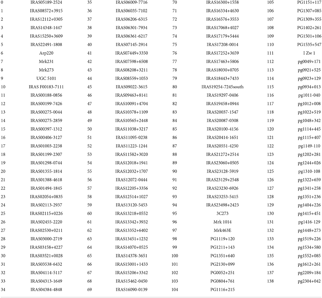
Table A1. Table of label numbering and galaxy names used in graphs, for reference.

FIGURE A1

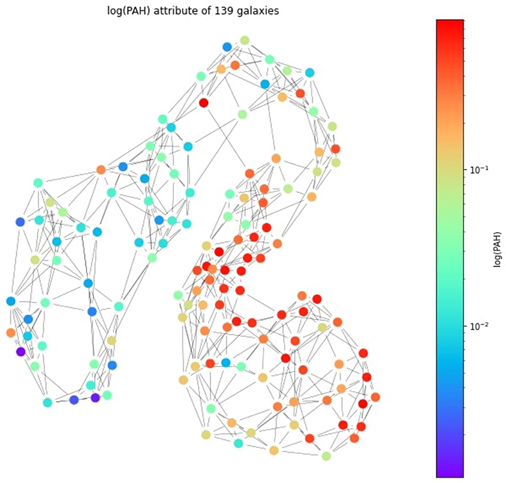
Figure A1. The PAH feature distribution on the graph.