Dynamics of heterogeneous population due to spatially distributed parameters and an ideal free pair

1. Introduction

The life history of most organisms depends on their dispersal strategy and resource distribution, which is the most important and obvious feature of ecology. Most of the time, their ecological impact and progression remain inadequately understood. The question that attracts most researchers is how individual organisms choose their habitat in the ecological niche. At this point, reaction-diffusion models can be used for interacting biological species in an isolated confined habitat that is highly adapted for capturing species' bio-geographic properties. Numerous new theoretical research in the field of mathematical ecology have been conducted on the reaction-diffusion problem (refer to, e.g., [1–6] and references therein) that suggest in many cases the uniform and non-uniform ideal free distribution. The key idea of ideal free distribution is that the individual has an extensive understanding of the environment. They can freely diffuse where they evaluate them-self in order to optimize their fitness, without any cost. The concept of ideal free distribution was laid out in Cantrell et al. [5], which signifies any movement from this dispersed system will diminish the fitness of the moving organism. Spatially heterogeneous, but temporary constant ideal free distribution is estimated as the solution of the model. In this context, for model dispersal, there were various promising approaches (refer to, e.g., [4–6]) that provide the ideal free distribution as the equilibrium solution of the dynamical model.

However, the most crucial problem in heterogeneous environments is that the strategy of diffusion, which is adopted from any physical system, presumes enormous migration of organisms to the areas of poor available resources [3, 7]. The migration transport is considered proportional to the gradient of population density itself. In this situation, species can be preordained to extinction. As in classical diffusion, species are uniformly distributed over the space with the increase of the diffusion coefficient. However, ideal free distribution corresponds to the equal distribution of available resources at each spatial location. Classical diffusion cannot correspond to the ideal free dispersal in a spatially non-homogeneous environment. As a remedy to this, in our study, we have considered an alternative take out type of diffusion strategy, named resource-based diffusion [8, 9] along with a positive and smooth distribution function, which is individual for each population. In this migration pattern, the diffusive transport is considered proportional to the gradient of population density per unit resource instead of the carrying capacity studied in Braverman and Braverman [4] and Korobenko and Braverman [10].

The evolutionary advantage of various diffusion tactics on the outcome of competition coefficients on the model parameters was studied in Kamrujjaman [11]. The major outcome of this study was that the mutual coexistence of species and destruction of one by others, as well as considering the case for which both species are managed confirms the ideal free pair. The case of weak competition for two competing species was studied in Kamrujjaman [12] where the diffusion strategy of two competing species is considered different, the first species following the resource-base diffusion, whereas others disperse randomly. The study concluded that the resource-based diffusion strategy has an evolutionary advantage compared to regular diffusion. Also, it was found that when two strategies, adopted by the competing species, were combined, both species were able to coexist and an ideal free pair was attained.

Moreover, competition between organisms is usually depicted by the predator-prey and Lotka system. The Lotka-Volterra system with random diffusion has been discussed in the literature [7, 13, 14] throughout the last two decades. Partial resource sharing described by a Lotka system with competition parameters between zero and one was studied in Braverman and Kamrujjaman [15]. They investigated how the diffusion coefficients, as well as the competition coefficients, can affect whether a possible interaction is a coexistence or competitive exclusion. Furthermore, two species striving for the same resource are unable to coexist. Spatial heterogeneity, which is defined by the environment's resource capacity, intrinsic growth rate, inter-specific competition coefficient, and spatially distributed diffusion strategies, can alter the scenario.

Inspired by the overhead discussion, in this study, we have studied a two species compete model, where the main aim behind it is based on different imposed diffusion strategies and the tensity of competition coefficient on their growth function. We will study the existence of global stability both for competitive exclusion and coexistence of the model, without imposing additional conditions on the model parameter in which ideal free pair exists in competition.

2. Mathematical model

Let us now define the well known growth functions that we want to define in our generalized reaction-diffusion system:

Gilpin-Ayala growth [16]:

$\begin{array}{ll}F(x,u,K(x))=r(x)\left(1-{\left(\frac{u(t,x)}{K(x)}\right)}^{\theta }\right),0<\theta \le 1;& (2.1)\end{array}$

For θ = 1, the logistic growth is a particular case;

Gompertz growth [17]:

$\begin{array}{ll}F(x,u,K(x))=r(x)ln\left(\frac{K(x)}{u(t,x)}\right);& (2.2)\end{array}$

Food-limited growth [18]:

$\begin{array}{ll}F(x,u,K(x))=r(x)\frac{1-u(t,x)/K(x)}{1+\beta u(t,x)/K(x)},\beta >0.& (2.3)\end{array}$

In this study, we contemplate a couple of species competition models in mathematical ecology. Both species compete for the same basic resources at time t and location x, and early define the notation, Λ = Ω × (0, ∞) and ∂Λ = ∂Ω × (0, ∞). Both species are competing for the available natural resources in an isolated domain Ω and their diffusion strategies are similar according to two spatially distribution functions. This corresponds to the following non-linear system of equations with zero Neumann boundary conditions:

$\begin{array}{ll}\{\begin{array}{l}{u}_t=d_1\Delta \left(\frac{u(t,x)}{M(x)}\right)+r_1(x)u(t,x)f(x,u,v,M,N,K),\text{in }\Lambda ,\\ v_t=d_2\Delta \left(\frac{v(t,x)}{N(x)}\right)+r_2(x)v(t,x)f(x,v,u,N,M,K),\text{in }\Lambda ,\\ \nabla (u/M)·n=\nabla (v/N)·n=0,\text{on }\partial \Lambda ,\\ u(0,x)=u_0(x),v(0,x)=v_0(x),\text{in }\Omega .\end{array}& (2.4)\end{array}$

For spatially distributed positive functions M(x), N(x), and K(x), we assume that M(x) < K(x) and N(x) < K(x) for any x in a non-empty open domain. However, K(x) is the ultimate population density which is well known as the natural carrying capacity. The habitat Ω is defined as a bounded region in ℝⁿ, where n = 1, 2, or 3 with ∂Ω ∈ C^2+β, β > 0. The population densities of the two competing species are represented, respectively by the functions u(t, x) and v(t, x), where their migration rates are d₁ > 0 and d₂ > 0, respectively. The intrinsic growth rate of species is represented by the function r_i(x), (i = 1, 2), and it is bounded. We suppose that all functions belong to the class of $C^{1+\beta }(\overline{\Omega })$, β > 0 for any $x\in \overline{\Omega }$. As well as, throughout this study, we will assume that M(x) and N(x) satisfy

• distribution functions M(x) > 0 and N(x) > 0 are non-constant and Hölder continuous in Ω.

In the case of logistic growth, the system (2.4) can be presented in the following pattern

$\begin{array}{ll}\{\begin{array}{l}{u}_t=d_1\Delta \left(\frac{u(t,x)}{M(x)}\right)+r_1(x)u(t,x)\\ (1-\frac{u(t,x)+\mu (x)v(t,x)}{K(x)}),\text{ in }\Lambda ,\\ v_t=d_2\Delta \left(\frac{v(t,x)}{N(x)}\right)+r_2(x)v(t,x)\\ (1-\frac{\nu (x)u(t,x)+v(t,x)}{K(x)}),\text{ in }\Lambda ,\\ \nabla (u/M)·n=\nabla (v/N)·n=0,\text{ on }\partial \Lambda ,\\ u(0,x)=u_0(x),v(0,x)=v_0(x),\text{ in}\Omega .\end{array}& (2.5)\end{array}$

where

$\begin{array}{ll}\mu (x)=\frac{K(x)-M(x)}{N(x)},\nu (x)=\frac{K(x)-N(x)}{M(x)}.& (2.6)\end{array}$

In the past periods, most of the study of the competition model has been accomplished by considering constant competition coefficients [12, 15, 19] which belong to either 0 and 1 or greater than 1. In our study, we have designed our model by considering non-constant space dependent competition coefficient μ(x) and ν(x), which makes this study extremely novel and to the best of the authors' knowledge, until now no literature is available considering this type of space dependent competition coefficients. However, considering resource-based diffusion as a strategy for both competing species for generalized growth function is not investigated earlier in the literature.

Let us consider the growth functions as, g₁(x, u, v) = r₁uf(x, u, v, M, N, K) and g₂(x, u, v) = r₂vf(x, v, u, N, M, K). We next list the following assumptions on g₁ and g₂ which will be used throughout the article:

h1 g = (g₁, g₂) is quasimonotone nonincreasing in l₁ × l₂;

h2 g_i(·, u, v) is Hölder continuous in Ω and $f_i(x,·,·)\in C^2(l_1\times l_2)$, i = 1, 2;

h3 $f(x,u,v,M,N,K)=F(x,u+\frac{K-M}{N}v,K)$, and $f(x,v,u,N,M,K)=F(x,v+\frac{K-N}{M}u,K)$;

h4 f(x, M, N, M, N, K) = f(x, N, M, N, M, K) = F(x, K, K) = 0;

h5 F(x, u, M, N, K) is decreasing in u in a strictly monotonic manner;

h6 F(x, u, M, N, K) is increasing in K precisely in a strictly monotonic manner;

The most common instances of F(x, u, K) that satisfy the following properties are defined in (2.1)-(2.3). The property h5 of growth for the model's population densities does not satisfy for growth laws with the Allee effect [20].

Let us now introduce two new variables $m(t,x)=\frac{u(t,x)}{M(x)}$ and $w(t,x)=\frac{v(t,x)}{N(x)}$, and we get the above equivalent system of (2.4)

$\begin{array}{ll}\{\begin{array}{l}M(x)m_t=d_1\Delta m(t,x)+r_1(x)M(x)m(t,x)h(x,m,w,M,N,K),\\ \text{ in }\Lambda ,\\ N(x)w_t=d_2\Delta w(t,x)+r_2(x)N(x)w(t,x)h(x,w,m,N,M,K),\\ \text{ in }\Lambda ,\\ \nabla m·n=\nabla w·n=0,\text{ on }\partial \Lambda ,\\ m(0,x)=u_0(x)/M(x),w(0,x)=v_0(x)/N(x),\text{ in }\Omega .\end{array}& (2.7)\end{array}$

where h is a new function instead of f for new substitutions. For further analysis, we can consider either the problem (2.4) or (2.7) since both systems are equivalent.

In the present study, the main findings are as follows:

1. We demonstrate the global existence and uniqueness of the solution of the initial value system under some assumptions on the model parameters.

2. We investigate the global existence of the competition model in which the first species' resource function is proportional to its carrying capacity and the other is following a resource-based diffusion strategy by considering two main cases of competition coefficient: weak competition and strong competition.

3. We will find when M(x) + N(x) > K(x) i.e., μ(x), ν(x) < 1 (weak competition) then both species should survive in the competition and as t → ∞ the solution move toward (M, N) and form an ideal free pair.

4. Also, when M(x) + N(x) < K(x) i.e., μ(x), ν(x) > 1 (strong competition) no coexistence solution is possible and depending on the values of proportionally constant one of the species will survive in the battle.

5. In the case when both species follow the resource-based diffusion strategy, along with their positive distribution function and M(x) + N(x) ≥ K(x), they will attain an ideal free pair and both species should coexist.

6. We also present some numerical results both in one- and two-dimensional cases. In addition, we present the case of time periodic state with the same time period numerically to compare the time periodic cases which may occur for seasonal variation with the steady state case.

The manuscript is arranged as follows: the existence of the solution of the competition model for generalized growth functions is provided in Section 3. Section 4, reveals the existence of global and local stability under some conditions on the resource functions. Here, we have considered two cases: weak competition and strong competition, based on the values of space dependent competition coefficients. The main result of this study is also presented in this section. To see the efficacy of the model, the numerical computation both for the case of one dimension and two dimensions are presented in Section 5 in terms of a line graph, surface plots, trajectory plots, contour plots, and heat maps. Some numerical results for the time periodic state are also presented since it is very important for ecological consideration. Section 6, provides the concluding remarks of the study.

3. Existence and distinctiveness

To delineate the existence and uniqueness of u = u(t, x) with zero Neumann boundary conditions consider the following boundary value problem for the first equation of (2.4)

$\begin{array}{ll}\{\begin{array}{l}{u}_t=d_1\Delta \left(\frac{u(t,x)}{M(x)}\right)+r_1(x)u(t,x)f(x,u,v,M,N,K),\text{ in }\Lambda ,\\ \nabla (u/M)·n=0,\text{ on }\partial \Lambda ,\\ u(0,x)=u_0(x),\text{ in }\Omega .\end{array}& (3.1)\end{array}$

The following results are also discussed in Cantrell and Cosner [7] and Korobenko and Braverman [21]. It is to be mentioned that the proof of Lemma 1 and Lemma 2 are analogous to the proofs of Korobenko and Braverman [21], Theorem 1 and Theorem 2, where the authors considered two competing species competing for similar basic resources in the heterogeneous habitat with different diffusion strategies. The study was as follows: one species followed the carrying capacity-driven diffusion while others dispersed by the random movement for generalized symmetric growth function with μ(x) = ν(x) = 1.

Lemma 1. Korobenko and Braverman [21] Let g₁(x, u, v) = r₁uf(x, u, v, M, N, K) satisfy the property h2, h4, h5 and the initial condition of 3.1 be u₀(x) ∈ C(Ω), u₀(x) ≥ 0 in Ω and u₀(x) > 0 in some open, bounded, and non-empty domain Ω_s ⊂ Ω. Also let, all the the parameters are positive on $\overline{\Omega }$. Then there exists a unique positive solution u^*(x) of the system 3.1. Furthermore, if $\frac{M(x)}{K(x)}\equiv Constant$, then the only solution of problem 3.1 is u^*(x) = K(x), and as t → ∞ the solution converges to K(x), otherwise u^*(x) is different from K(x).

Similarly, we can also establish the existence and unique results for the second equation of (2.4) for v = v(t, x) with homogeneous Neumann boundary conditions as

$\begin{array}{ll}\{\begin{array}{l}{v}_t=d_2\Delta \left(\frac{u(t,x)}{N(x)}\right)+r_2(x)v(t,x)f(x,v,u,N,M,K),\text{ in }\Lambda ,\\ \nabla (v/N)·n=0,\text{ on }\partial \Lambda ,\\ v(0,x)=v_0(x),\text{ in }\Omega .\end{array}& (3.2)\end{array}$

Lemma 2. Korobenko and Braverman [21] Let g₂(x, u, v) = r₂vf(x, v, u, N, M, K) satisfy the property h2, h4, h5 and the initial condition of 3.1 be u₀(x) ∈ C(Ω), v₀(x) ≥ 0 in Ω and v₀(x) > 0 in some open, bounded, and non-empty domain Ω_s ⊂ Ω. Also let, all the parameters are positive on $\overline{\Omega }$. Then there exists a unique positive solution v^*(x) of the problem (3.2). Furthermore, if $\frac{N(x)}{K(x)}\equiv Constant$, then $\underset{t\to \infty }{\text{lim}}v(t,x)=K(x)$ otherwise $\underset{t\to \infty }{\text{lim}}v(t,x)=v^{*}(x)$ evenly in $x\in \overline{\Omega }$.

The following Theorem 1 establishes the existence and uniqueness of (2.4) for coupled systems of equations. Model (2.4) is a paragon that follows the monotone dynamical system [7, 22, 23]. Once substituting, m = u/M, and w = v/N it reduces into a system of regular diffusion. Where d₁/M and d₂/N represent space dependent positive smooth diffusion coefficients. Note that the following proof for (2.4) is analogous with Korobenko and Braverman [21] in Theorem 10, for μ = ν = 1.

Theorem 1. Let K(x), M(x), N(x) > 0 where M(x), N(x) < K(x) for any x in a non-empty open domain so that μ(x), ν(x) > 0 and g₁(x, u, v) = r₁uf(x, u, v, M, N, K) and g₂(x, u, v) = r₂vf(x, v, u, N, M, K) satisfy the property h1, h2, and h5 on $x\in \overline{\Omega }$. Then for any u₀(x), v₀(x) ∈ C(Ω) the problem (2.4) has a unique solution (u, v). Furthermore, if both initial functions are non-negative and non-trivial, then u(t, x) > 0 and v(t, x) > 0 for any t > 0.

Proof: To prove this, we enacted ([22], Theorem 8.7.2) to the problem (2.7), which is obtained after substitution $m=\frac{u(t,x)}{M(x)}$, and $w=\frac{v(t,x)}{N(x)}$, respectively.

To show the existence of non-trivial solutions, let us choose the following constants ρ_m and ρ_w such that

$\begin{array}{l}{\rho }_m\ge {\displaystyle \underset{(t,x)\in {𝔸}_1}{sup}}{u}_0(t,x)/M(x),\text{ and }{\rho }_w\ge {\displaystyle \underset{x\in \omega }{sup}}{v}_0(t,x)/N(x).\end{array}$

Then it is simple to check that the subsequent conditions of the theorem are satisfied.

$\begin{array}{ll}{g}_1(t,x,{\rho }_m,0,M,N,K)\le 0\le g_1(t,x,0,{\rho }_w,M,N,K).& (3.3)\end{array}$

$\begin{array}{ll}{g}_2(t,x,0,{\rho }_w,N,M,K)\le 0\le g_2(t,x,{\rho }_m,0,N,M,K).& (3.4)\end{array}$

So that f(t, x, ρ_m, 0, M, N, K) < 0 and f(t, x, 0, ρ_w, N, M, K) < 0, since f(x, Mm, Nw, M, N, K) and f(x, Nw, Mm, N, M, K) are monotonically nonincreasing in ℝ⁺. However, u(0, x) and v(0, x) are bounded in $\overline{\Omega }$, and M(x) and N(x) are bounded from below, so we have $\underset{x\in \Omega }{sup}\frac{u(0,x)}{M(t,x)}<\infty$, and $\underset{x\in \Omega }{sup}\frac{v(0,x)}{N(x)}<\infty$, respectively.

The conditions (3.3) and (3.4) satisfy the conditions (refer to, [22], Theorem 8.7.2, Equation 8.7.4) for the functions g₁ and g₂ defined above. Therefore, we arrive at the conclusion of the theorem that for any non-trivial and non-negative (u₀(x), v₀(x)) such that ρ_m and ρ_w specified above satisfy

$\begin{array}{l}\left(\frac{u_0(x)}{M(x)},\frac{v_0(x)}{N(x)}\right)\in {\text{S}}_{\rho }:=\{(m,w)\in C\left([0,\infty )\times \overline{\Omega }\right)\\ \times C\left([0,\infty )\times \overline{\Omega }\right):(0,0)\\ \le (m,w)\le ({\rho }_m,{\rho }_w)\}.\end{array}$

Where $C([0,\infty )\times \overline{\Omega })$ denotes the class of continuous functions on $[0,\infty )\times \overline{\Omega }$. Accordingly, from (refer to, [22], Theorem 8.7.2) all of the requirements have been met, so the unique solution (m, w) of (2.7) has existed and it is positive. Apparently, the unique positive solution of (2.4) is (u, v) = (Mm, Nw). Thus, the solution (u, v) is positive and unique.□

As a system (2.4) as well as (2.7) is a sample of the monotone dynamical system [7, 22, 23]. For further analysis of the model's equilibrium solutions, we will apply the following theorem of the monotone dynamical system that is provided in Korobenko and Braverman [21], Theorem 16.

Lemma 3. If the trivial equilibrium of (2.4) is not stable as well as the repeller, then certainly one of the subsequent three situations are stand from a specified set:

(i) a positive and stable coexistence of (2.4) will sustain,

(ii) all positive and stable solution either converges to (u^*, 0) as t → ∞,

(iii) all positive and stable solution either converges to (0, v^*) as t → ∞.

4. Analysis of steady states

In this part of the study, we will explore the stability of the following equilibrium states of the system (2.4): (u^*(x), 0), (0, v^*(x)) named semi-trivial equilibria, which corresponds to a situation where only one species survives in the competition and the other species dies out. The trivial equilibrium (0, 0), when both species leave the area and the coexistence equilibria (u_e(x), v_e(x)) while both semi-trivial, as well as the trivial solution, are unstable. As we know, u(t, x) and v(t, x) are the solutions of (2.4) for all t > 0. Also, we describe our main results.

Lemma 4. The (0, 0) equilibrium of the system (2.4) is unstable and repelling.

Proof: Let us consider the system (2.7) around the origin and the associated eigenvalue problem of the corresponding problem is

$\begin{array}{ll}\{\begin{array}{l}{d}_1\Delta \varphi (x)+r_1\varphi (x)M(x)h(x,0,0,M,N,K)=\sigma \varphi (x),\\ \text{ in }\Omega ,\nabla \varphi ·n=0,\text{ on }\partial \Omega ,\\ d_2\Delta \psi (x)+r_2\psi (x)N(x)h(x,0,0,N,M,K)=\sigma \psi (x),\\ \text{ in }\Omega ,\nabla \psi ·n=0,\text{ on }\partial \Omega .\end{array}& (4.1)\end{array}$

The principal eigenvalue of the first equation of (4.1) is expressed by following the variational characterization of the eigenvalues ([7], Theorem 2.1) as

$\begin{array}{l}{\sigma }_1={\displaystyle \underset{\varphi \ne 0,\varphi \in W^{1,2}}{sup}}\\ \frac{-\underset{\Omega }{\int }{d}_1|\nabla \varphi (x){|}^{2}dx+\underset{\Omega }{\int }{r}_{1}M(x){\varphi }^2(x)h(x,0,0,M,N,K)dx}{\underset{\Omega }{\int }{\varphi }^2(x)dx}.\end{array}$

For non-trivial positive constant function ϕ(x), we get

$\begin{array}{l}{\sigma }_1\ge \frac{1}{|\Omega |}{\displaystyle \underset{\Omega }{\int }}{r}_{1}M(x)h(x,0,0,M,N,K)dx>0,\\ \text{ since }h(x,0,0,M,N,K)>0.\end{array}$

and the zero equilibrium (0, 0) of (2.4) is not stable.

To prove that (0, 0) of (2.4) is a repeller, i.e., assuming u₀, v₀ being the neighborhood of the equilibrium point (0, 0), then all solutions move away from (0, 0) as t approaches infinity.

Let $\delta =min\left\{\underset{x\in \Omega }{inf}\frac{K}{4},\underset{x\in \Omega }{inf}\frac{KN}{4(K-M)},\underset{x\in \Omega }{inf}\frac{MK}{4(K-N)}\right\}>0$, u₀(x) ≥ 0 and v₀(x) ≥ 0 be such that u₀(x) < δ, v₀(x) < δ for (u₀(x), v₀(x)) ≠ (0, 0). Adding the foremost equations of the system (2.4) and integrate over Ω and applying homogeneous Neumann boundary conditions, we get

$\begin{array}{ll}\begin{array}{l}\frac{d}{dt}{\displaystyle \underset{\Omega }{\int }}(u(t,x)+v(t,x))dx={\displaystyle \underset{\Omega }{\int }}[r_1(x)uf(x,u,v,M,N,K)\\ +r_2(x)vf(x,v,u,N,M,K)]dx.\end{array}& (4.2)\end{array}$

Note that, $\gamma =min\left\{\underset{x\in \Omega }{inf}{r}_1(x),\underset{x\in \Omega }{inf}{r}_2(x)\right\}>0$ and on condition, u ≤ δ and v ≤ δ there holds

$\frac{d}{dt}{\displaystyle \underset{\Omega }{\int }}(u(t,x)+v(t,x))dx\ge \frac{\gamma }{2}{\displaystyle \underset{\Omega }{\int }}(u(t,x)+v(t,x))dx.$

Now applying Gronwall's lemma we have

${\displaystyle \underset{\Omega }{\int }}(u(t,x)+v(t,x))dx\ge e^{\gamma t/2}{\displaystyle \underset{\Omega }{\int }}(u_0(x)+v_0(x))dx.$

As $\underset{\Omega }{\int }(u_0(x)+v_0(x))dx>0$, then $\underset{\Omega }{\int }(u(t,x)+v(t,x))dx$ expands exponentially with time goes as far as u ≤ δ and v ≤ δ. Hence there exists t₀ > 0 so that u(t₀, x) > δ and v(t₀, x) > δ for some x ∈ Ω and the equilibrium point (0, 0) is a repeller.□

The functions u^* and v^* are the solutions to the preceding elliptic boundary value problems, which are straightforward to understand:

$\begin{array}{l}{d}_1\Delta \left(\frac{u^{*}(x)}{M(x)}\right)+r_1(x)u^{*}(x)f(x,u^{*},0,M,N,K)=0,\\ \text{ in }\Omega ,\frac{\partial (u^{*}/M)}{\partial n}=0,\text{ on }\partial \Omega ,& (4.3)\end{array}$

$\begin{array}{l}{d}_2\Delta \left(\frac{v^{*}(x)}{N(x)}\right)+r_2(x)v^{*}(x)f(x,v^{*},0,N,M,K)=0,\\ \text{ in }\Omega ,\frac{\partial (v^{*}/N)}{\partial n}=0,\text{ on }\partial \Omega ,& (4.4)\end{array}$

respectively.

Lemma 5. Let f satisfy h1-h6, r₁(x) ≡ r₁, r₂(x) ≡ r₂ are constant and K(x) ≢ constant. Then a unique positive solution v^*(x) of (4.4) will exist, so that

$\begin{array}{l}{r}_2{\displaystyle \underset{\Omega }{\int }}f(x,v^{*},0,N,M,K)K(x)dx\equiv \\ r_2{\displaystyle \underset{\Omega }{\int }}F(x,v^{*}(x),K(x))K(x)dx>0.& (4.5)\end{array}$

Proof: Integrating (4.4) over the domain Ω and applying the corresponding boundary conditions which implies $d_2\underset{\Omega }{\int }\Delta v^{*}(x)dx=0$ and we obtain using h3 for g

$\begin{array}{ll}{\displaystyle \underset{\Omega }{\int }}{r}_2{v}^{*}(x)F(x,v^{*},K)dx=0.& (4.6)\end{array}$

Integrating the equality and using the Mean Value Theorem with property h4

$\begin{array}{l}{r}_2{v}^{*}(x)F(x,v^{*},K)=r_2(v^{*}-K)(F(x,v^{*},K)-F(x,K,K))\\ +r_{2}K(x)F(x,v^{*},K)\\ =r_2{(v^{*}-K)}^2{F}_v(x,\xi ,K)\\ +r_{2}K(x)F(x,v^{*},K)\end{array}$

we have

$\begin{array}{l}{r}_2{\displaystyle \underset{\Omega }{\int }}K(x)F(x,v^{*}(x),K(x))dx=\\ -{\displaystyle \underset{\Omega }{\int }}{F}_v(x,\xi ,K(x)){(v^{*}(x)-K(x))}^{2}dx>0.& (4.7)\end{array}$

where ξ(x) lies in between v^*(x) and K(x). Here the right-hand side is positive unless v^*(x) ≡ K(x) ≡ constant, since F_v < 0 due to h5, which completes the proof.□

Remark 1. Note that for any v ≤ K the properties h4 and h5 result in f(x, v, 0, N, M, K) ≥ 0. As a result, in an integral sense the inequality (4.5) can be regarded as the condition v^* < K(x).

Lemma 6. Let f satisfies h1-h6 and r₁(x) ≡ r₁, r₂(x) ≡ r₂ are constant and $\frac{K(x)}{M(x)}\equiv \beta >0$. Then the semi-trivial equilibrium (0, v^*(x)) of (2.4) is unstable if there exists non-constant M(x), N(x), and K(x) such that (M(x) + N(x)) ≥ K(x) i.e., μ(x) ≤ 1 in a non-empty open domain Ω_s ⊆ Ω.

Proof: First taking the linearization of (2.4) over (0, v^*(x)).

$\begin{array}{l}\{\begin{array}{l}\frac{\partial u}{\partial t}=d_1\Delta \left(\frac{u(t,x)}{M(x)}\right)+r_{1}u(t,x)f(x,0,v^{*},M,N,K),\\ (t,x)\in \Lambda ,\frac{\partial (u/M)}{\partial n}=0,x\in \partial \Omega ,\\ \frac{\partial v}{\partial t}=d_2\Delta \left(\frac{v(t,x)}{N(x)}\right)\\ +r_{2}v(t,x)f(x,v^{*},0,N,M,K)\\ +r_2{v}^{*}{f}_u(x,v^{*},0,N,M,K)u(t,x)\\ +r_2{v}^{*}{f}_v(x,v^{*},0,M,N,K)v(t,x),(t,x)\in \Lambda ,\\ \frac{\partial (v/N)}{\partial n}=0,x\in \partial \Omega .\end{array}\end{array}$

and study the corresponding eigenvalue problem for u

$\begin{array}{ll}\{\begin{array}{l}{d}_1\Delta \left(\frac{\varphi (x)}{M(x)}\right)+r_1\varphi (x)f(x,0,v^{*},M,N,K)=\sigma \varphi (x),x\in \Omega ,\\ \frac{\partial (\varphi /M)}{\partial n}=0,x\in \partial \Omega .\end{array}& (4.8)\end{array}$

If the principal eigenvalue is positive then (0, v^*) is unstable. Consider (4.8) and according to Cantrell and Cosner [7], Theorem 2.1, its principal eigenvalue is presented as

$\begin{array}{l}{\sigma }_1={\displaystyle \underset{\varphi \ne 0,\varphi \in W^{1,2}}{sup}}\\ \frac{-\underset{\Omega }{\int }{d}_1|\nabla (\varphi /M){|}^{2}dx+\underset{\Omega }{\int }\frac{r_1}{M}{\varphi }^2(x)f(x,0,v^{*},M,N,K)dx}{\underset{\Omega }{\int }\left(\frac{{\varphi }^2}{M}\right)dx}.\end{array}$

Letting ϕ(x) = K(x) and using the property h3

$\begin{array}{l}{\sigma }_1\ge \frac{\underset{\Omega }{\int }{r}_{1}K(x)F(x,\frac{K-M}{N}{v}^{*},K)dx}{\underset{\Omega }{\int }K(x)dx}\\ \ge \frac{r_1\underset{\Omega }{\int }K(x)F(x,v^{*},K)dx}{\underset{\Omega }{\int }K(x)dx},\text{ since }\mu (x)\equiv \frac{K(x)-M(x)}{N(x)}\\ \le 1\text{ for any }x\in {\Omega }_s\subseteq \Omega .& (4.9)\end{array}$

Thus, σ₁ > 0 using (4.5) in Lemma 5, which completes the proof.□

Lemma 7. Let f satisfies h1-h6 and r₁(x) ≡ r₁, r₂(x) ≡ r₂ are constant and $\frac{K(x)}{M(x)}\equiv \beta >0$. Then the semi-trivial equilibrium (K, 0) of (2.4) is unstable if there exists non-constant M(x), N(x), and K(x) such that (M(x) + N(x)) ≥ K(x) i.e., ν(x) ≤ 1 in a non-empty open domain Ω_s ⊆ Ω.

Proof: Analogous to Lemma 6, examine the associated eigenvalue problem of the linearized second equations of (2.4) around (K, 0) and we obtain

$\begin{array}{l}{d}_2\Delta \left(\frac{\psi (x)}{N(x)}\right)+r_2\psi (x)f(x,0,K,N,M,K)=\sigma \psi (x),x\in \Omega ,\\ \frac{\partial (\psi /N)}{\partial n}=0,x\in \partial \Omega .& (4.10)\end{array}$

Consider the Equation (4.10) and according to Cantrell and Cosner [7], the corresponding principal eigenvalue is stated as

$\begin{array}{l}{\sigma }_1={\displaystyle \underset{\psi \ne 0,\psi \in W^{1,2}}{sup}}{d}_2\\ \frac{-\underset{\Omega }{\int }|\nabla \psi (x)/N{|}^{2}dx+\underset{\Omega }{\int }{r}_2\frac{{\psi }^2}{N}f(x,0,K,N,M,K)dx}{\underset{\Omega }{\int }\left(\frac{{\psi }^2}{N}\right)dx}.\end{array}$

On substituting ψ(x) = N(x) and using h3, the principal eigenvalue is

${\sigma }_1\ge \frac{r_2\underset{\Omega }{\int }NF(x,\frac{K-N}{M}K,K)dx}{\underset{\Omega }{\int }{K}^2(x)dx}.$

Since, $F(x,\frac{K-N}{M}K,K)=\frac{M(x)-K(x)+N(x)}{M(x)}>0$ for M(x) + N(x) > K(x), also N(x) > 0. Therefore, σ₁ > 0 and (K, 0) of (2.4) is unstable.□

Since (0, v^*(x)) and (K(x), 0) are not stable as far as (M(x) + N(x)) > K(x) (refer to, Lemma 6 and Lemma 7), they are not asymptotically stable. Also from Lemma 4, (0, 0) or trivial equilibrium is unstable and repeller. Therefore, according to strong monotone dynamical system [7, 22, 23] the coexistence equilibrium (u_e(x), v_e(x)) is globally asymptotically stable so as to (M(x) + N(x)) ≥ K(x) for all x. Since system (2.4) is an example of a strongly monotone dynamical system, which represents the following Theorem 2.

Theorem 2. Let the functions g₁(x, u, v) = r₁uf(x, u, v, M, N, K) and g₂(x, u, v) = r₂vf(x, v, u, N, M, K) satisfy h1-h6. Also, let r₁(x) ≡ r₁, r₂(x) ≡ r₂ are constant and $\frac{K(x)}{M(x)}\equiv \beta >0$. Then the coexistence equilibrium (u_e(x), v_e(x)) of the system of Equations (2.4) is globally asymptotically stable if (M(x) + N(x)) > K(x) for any x in a non-empty open domain. Also if K ≡ constant then the equilibrium (u_e(x), v_e(x)) is globally asymptotically stable when M(x) + N(x) ≡ K. That is, for any $u_0,v_0\in C(\overline{\Omega })$ which is non-negative and non-trivial, the solution (u, v) of (2.4) satisfies

$\begin{array}{l}(u,v)\to (u_e(x),v_e(x)),ast\to \infty .\end{array}$

Corollary 1. Let the functions g₁(x, u, v) = r₁uf(x, u, v, M, N, K) and g₂(x, u, v) = r₂vf(x, v, u, M, N, K) satisfy h1-h6. Also if M, N, K all are constants and (M + N) > K then the coexistence equilibrium (M, N) of the system of equations (2.4) is globally asymptotically stable. That is, for any $u_0,v_0\in C(\overline{\Omega })$ which is non-negative and non-trivial, the solution (u, v) of (2.4) satisfies

$\begin{array}{l}(u,v)\to (M,N),ast\to \infty \end{array}$

uniformly in $x\in \overline{\Omega }$.

Next, in the following result, it is shown that there is no coexistence for strong competition, depending on the relations between M(x), N(x), and K(x). In this case, competitive exclusion is expected.

Lemma 8. Let f satisfies h1-h6 and M(x), N(x), K(x) are non-constant. If (M(x) + N(x)) ≤ K(x) for any x ∈ Ω, i.e., μ(x), ν(x) ≥ 1 in a non-empty open domain Ω_s ⊆ Ω with r₁(x) ≡ r₁, r₂(x) ≡ r₂ are constant, $\frac{K(x)}{M(x)}\equiv \beta >0$, then there is no coexistence steady state (u_e, v_e) of the system (2.4).

Proof: Suppose to the contrary, let us assume there exists a strictly positive equilibrium solution (u_e(x), v_e(x)) of (2.4) and we will present that the assumption provides a conflict. So, the solution (u_e(x), v_e(x)) satisfies the governing equations

$\begin{array}{ll}\{\begin{array}{l}{d}_1\Delta \left(\frac{u_e(x)}{M(x)}\right)+r_1{u}_e(x)f(x,u_e,v_e,M,N,K)=0,\text{ in }\Omega ,\\ \frac{\partial (u_e/M)}{\partial n},\text{ on }\partial \Omega ,\\ d_2\Delta \left(\frac{v_e(x)}{N(x)}\right)+r_2{v}_e(x)f(x,v_e,u_e,N,M,K)=0,\text{ in }\Omega ,\\ \frac{\partial (v_e/N)}{\partial n}=0,\text{ on }\partial \Omega .\end{array}& (4.11)\end{array}$

After dividing by r₁r₂ in each of the first two equations in (4.11) and adding them as well as imposing h3 for f, we get

$\begin{array}{l}\frac{d_1}{r_1}\Delta \left(\frac{u_e(x)}{M(x)}\right)+\frac{d_2}{r_2}\Delta \left(\frac{v_e(x)}{N(x)}\right)+u_e(x)F(x,u_e+\mu (x)v_e,K)\\ +v_e(x)F(x,v_e+\nu (x)u_e,K)=0.\end{array}$

Integrating over Ω and applying Numann boundary conditions in (4.11), we have

$\begin{array}{l}0={\displaystyle \underset{\Omega }{\int }}\left[u_{e}F(x,u_e+\mu (x)v_e,K)+v_{e}F(x,v_e+\nu (x)u_e,K)\right]dx\\ <{\displaystyle \underset{\Omega }{\int }}\left[u_{e}F(x,u_e+\mu (x)v_e,K)+\mu (x)v_{e}F(x,u_e+\mu (x)v_e,K)\right]dx\\ ={\displaystyle \underset{\Omega }{\int }}(u_e+\mu (x)v_e)F(x,u_e+\mu (x)v_e,K)dx.\end{array}$

since μ(x)F(x, u_e + μ(x)v_e, K) > F(x, v_e + ν(x)u_e, K), for ν(x) > μ(x). Thus

$\begin{array}{ll}{\displaystyle \underset{\Omega }{\int }}(u_e+\mu (x)v_e)F(x,u_e+\mu (x)v_e,K)dx>0.& (4.12)\end{array}$

Integrating the equality

$\begin{array}{l}(u_e+\mu (x)v_e)F(x,u_e+\mu (x)v_e,K)=F(x,u_e+\mu (x)v_e,K)\\ (u_e+\mu (x)v_e-K)\\ +K(x)F(x,u_e+\mu (x)v_e,K)\end{array}$

over Ω using (4.12) we get,

$\begin{array}{l}0<{\displaystyle \underset{\Omega }{\int }}F(x,u_e+\mu (x)v_e,K)(u_e+\mu (x)v_e-K)dx\\ +{\displaystyle \underset{\Omega }{\int }}K(x)F(x,u_e+\mu (x)v_e,K)dx.& (4.13)\end{array}$

The Mean Value Theorem and F(x, K, K) = 0 by h4 imply

$\begin{array}{l}F(x,u_e+\mu (x)v_e,K)=F(x,u_e+\mu (x)v_e,K)-F(x,K,K)\\ =F_v(x,\xi ,K)(u_e+\mu (x)v_e-K)& (4.14)\end{array}$

where ξ is between u_e + μ(x)v_e and K for each (t, x) ∈ Λ. Using (4.14), inequality (4.15) can be rewritten as

$\begin{array}{l}{\displaystyle \underset{\Omega }{\int }}K(x)F(x,u_e+\mu (x)v_e,K)dx>\\ -{\displaystyle \underset{\Omega }{\int }}{F}_v(x,\xi ,K){(u_e+\mu (x)v_e-K)}^{2}dx.& (4.15)\end{array}$

and the last inequality is strictly positive and excludes the possibility of u_e + μ(x)v_e ≡ K where F_v < 0 due to h5. Thus, we have to consider the following case.

Let u_e + μ(x)v_e ≢ K in some nonempty open domain, where μ(x), ν(x) ≥ 1. Consider the eigenvalue problem

$\begin{array}{l}{d}_1\Delta \left(\frac{\varphi (x)}{M(x)}\right)+r_1\varphi (x)F(x,u_e+\mu (x)v_e,K)=\sigma \varphi (x),x\in \Omega ,\\ \frac{\partial (\varphi /M)}{\partial n}=0,x\in \partial \Omega .& (4.16)\end{array}$

According to Cantrell and Cosner [7], Theorem 2.1, the corresponding principal eigenvalue is presented as

$\begin{array}{l}{\sigma }_1={\displaystyle \underset{\varphi \ne 0,\varphi \in W^{1,2}}{sup}}\\ \frac{-\underset{\Omega }{\int }{d}_1|\nabla (\varphi /M){|}^{2}dx+r_1\underset{\Omega }{\int }\frac{{\varphi }^2}{M}F(x,u_e+\mu (x)v_e,K)dx}{\underset{\Omega }{\int }({\varphi }^2/M)dx}\end{array}$

Letting ϕ(x) = K(x) and applying (4.15), we obtain

$\begin{array}{l}{\sigma }_1\ge \frac{r_1\underset{\Omega }{\int }K(x)F(x,u_e+\mu (x)v_e,K)dx}{\underset{\Omega }{\int }K(x)dx}>0,\\ \text{ since }K/M\equiv constant.& (4.17)\end{array}$

Since 0 is always a principal eigenvalue of (4.16) along with a positive principal eigenfunction, which contradicts the positivity of σ₁ > 0.□

Remark 2. The Lemma 8 is also valid for proportional growth rates $\frac{r_1(x)}{r_2(x)}=\alpha >0$, since r₂(x) can be involved as a part of function F.

Remark 3. If all the functions M, N, and K are constants then always there exists a coexistence solution (M, N) of the system (2.4) and the solution is globally stable.

Lemma 9. Let f satisfy h1-h6 and M(x), N(x), K(x) are non-constant. If (M(x) + N(x)) ≤ K(x) for any x ∈ Ω, i.e., μ(x) ≥ 1 in a non-empty open domain Ω_s ⊆ Ω with r₁(x) ≡ r₁, r₂(x) ≡ r₂ are constant, $\frac{K(x)}{M(x)}\equiv \beta >0$, then the semi-trivial steady state (K, 0) of the system (2.4) is locally asymptotically stable.

Proof: Similar to the proof of Lemma 7, let us study the associated eigenvalue problem of the linearized second equations of (2.4) around (K, 0), then according to Cantrell and Cosner [7], Theorem 2.1 the principal eigenvalue is given by

$\begin{array}{l}{\sigma }_1={\displaystyle \underset{\psi \ne 0,\psi \in W^{1,2}}{sup}}{d}_2\\ \frac{-\underset{\Omega }{\int }|\nabla \psi (x)/N{|}^{2}dx+\underset{\Omega }{\int }{r}_2\frac{{\psi }^2}{N}f(x,0,K,N,M,K)dx}{\underset{\Omega }{\int }\left(\frac{{\psi }^2}{N}\right)dx}.\end{array}$

Upon putting ψ(x) = N(x) and using h3, the principal eigenvalue is

${\sigma }_1\ge \frac{r_2\underset{\Omega }{\int }NF(x,\frac{K-N}{M}K,K)dx}{\underset{\Omega }{\int }N(x)dx}.$

Since, $F(x,\frac{K-N}{M}K,K)=1-\frac{(\frac{K-N}{M})K}{K}=\frac{M(x)-K(x)+N(x)}{M(x)}<0$ for M(x) + N(x) < K(x), also N(x) > 0. Therefore, σ₁ < 0 and semi-trivial equilibrium (K, 0) of (2.4) is locally stable.□

In a similar way, we can prove (0, v^*) is locally stable if (M(x) + N(x)) ≤ K(x) for any x ∈ Ω, i.e., ν(x) ≥ 1 in a non-empty open domain Ω_s ⊆ Ω with r₁(x) ≡ r₁, r₂(x) ≡ r₂ are constant, $\frac{K(x)}{M(x)}\equiv \beta >0$.

As Lemma 4 is still valid. From Lemma 8 and Lemma 9, we can state the consequent Theorem 3, represents the local existence of one semi-trivial steady state controlling the initial conditions.

Theorem 3. Let the functions g₁(x, u, v) = r₁uf(x, u, v, M, N, K) and g₂(x, v, u) = r₂vf(x, v, u, N, M, K) satisfy h1-h6 and K(x) ≢ constant. Also, let r₁(x) ≡ r₁, r₂(x) ≡ r₂ are constant and $\frac{K(x)}{M(x)}\equiv \beta >0$. Then either the equilibrium (K(x), 0) or the equilibrium (0, v^*(x)) of the system of equations (2.4) is locally asymptotically stable if (M(x) + N(x)) ≤ K(x) for any x ∈ Ω. That is, depending on $u_0,v_0\in C(\overline{\Omega })$, the solution (u, v) of (2.4) satisfies

$\begin{array}{l}\text{either}(u,v)\to (K,0),\text{ or }(u,v)\to (0,v^{*}),ast\to \infty \end{array}$

uniformly in $x\in \overline{\Omega }$.

Corollary 2. Let the functions g₁(x, u, v) = r₁uf(x, u, v, M, N, K) and g₂(x, v, u) = r₂vf(x, v, u, N, M, K) satisfy h1-h6 and K(x) ≡ constant. Then either the equilibrium (K(x), 0) or the equilibrium (0, v^*(x)) of the system of equations (2.4) is locally asymptotically stable if M(x) + N(x) < K for any x ∈ Ω. That is, depending on $u_0,v_0\in C(\overline{\Omega })$, the solution (u, v) of (2.4) satisfies

$\begin{array}{l}\text{either}(u,v)\to (K,0),\text{ or }(u,v)\to (0,v^{*}),ast\to \infty \end{array}$

uniformly in $x\in \overline{\Omega }$.

Lemma 10. Let the growth function f satisfy h1-h6, r₁(x) ≡ r₂(x) ≡ r are constant and K(x) ≢ constant. If (u^*, 0) and (0, v^*) are the semi-trivial solution of (4.3) and (4.4), respectively and μ, ν ∈ (0, 1) then

$\begin{array}{l}r{\displaystyle \underset{\Omega }{\int }}f(x,0,v^{*},0,M,N,K)M(x)dx\equiv \\ r{\displaystyle \underset{\Omega }{\int }}F(x,v^{*}(x),M,N,K)M(x)dx>0,& (4.18)\end{array}$

and

$\begin{array}{l}r{\displaystyle \underset{\Omega }{\int }}f(x,0,u^{*},N,M,K)N(x)dx\equiv \\ r{\displaystyle \underset{\Omega }{\int }}F(x,v^{*}(x),N,M,K)N(x)dx>0.& (4.19)\end{array}$

Proof: Let us assume, $N_1=\underset{\Omega }{\int }M(x)dx$ and $N_2=\underset{\Omega }{\int }N(x)dx$ where r₁(x) ≡ r₂(x) ≡ r.

Denote,

$\begin{array}{l}{a}^{*}=min\left\{\frac{N_1}{\underset{\Omega }{\int }(\frac{M(x)v^{*}(x)}{K(x)})dx},1\right\}\in (0,1)\end{array}$

If μ ∈ (0, a^*) then,

$\begin{array}{l}{\displaystyle \underset{\Omega }{\int }}\frac{M(x)v^{*}(x)\mu (x)}{K(x)}dx<N_1\\ \Rightarrow {\displaystyle \underset{\Omega }{\int }}r\frac{M(x)v^{*}(x)\mu (x)}{K(x)}dx<r{\displaystyle \underset{\Omega }{\int }}M(x)dx,\\ \text{where }\mu (x)\in (0,1)\text{ and }r\text{ is constant}\\ \Rightarrow r{\displaystyle \underset{\Omega }{\int }}\left(1-\frac{\mu v^{*}}{K}\right)Mdx>0\\ \Rightarrow r{\displaystyle \underset{\Omega }{\int }}g(x,v^{*},0,M,N,K)Mdx>0.\end{array}$

Applying property h3 for f, we get, $r\underset{\Omega }{\int }F(x,v^{*},M,N,K)Mdx>0.$

Now if (u^*, 0) is a semi-trivial equilibrium of (4.3) and $a^{**}=min\left\{\frac{N_2}{\underset{\Omega }{\int }\left(\frac{N(x)v^{*}(x)}{K(x)}\right)dx},1\right\}\in (0,1)$ than for ν ∈ (0, a^**) ∈ (0, 1), applying the same procedure as before we can find,

$\begin{array}{l}r{\displaystyle \underset{\Omega }{\int }}F(x,u^{*},N,M,K)Ndx>0.\end{array}$

   □

Now we will analyze the case of the ideal free pair when M(x), N(x), and K(x) are space dependent and non-proportional to each other. By direct substitution of $\mu (x)=\frac{K(x)-M(x)}{N(x)}$ and $\nu (x)=\frac{K(x)-N(x)}{M(x)}$ it is easy to check that (M, N) is the solution of the system (2.4). Now we will establish this coexistence steady state via the instability of both (u^*, 0) and (0, v^*).

Lemma 11. Let f satisfies h1-h6 and M(x), N(x), and K(x) are non-constant and linearly independent. If r₁(x) ≡ r₂(x) ≡ r are constant and (M(x) + N(x)) ≥ K(x) for any x ∈ Ω, then the semi-trivial steady state (0, v^*) of the system (2.4) is unstable.

Proof: Assume the linearized equations of the problem (2.4) for the first equation around (0, v^*), then the associated eigenvalue problem for u is,

$\begin{array}{l}{d}_1\Delta \left(\frac{\varphi (x)}{M(x)}\right)+r_1\varphi (x)f(x,0,v^{*},M,N,K)=\sigma \varphi (x),\\ \in \Omega ,\frac{\partial (\varphi /M)}{\partial n}=0,x\in \partial \Omega .& (4.20)\end{array}$

According to Cantrell and Cosner [7], Theorem 2.1, the principal eigenvalue of (4.20) is represented as

$\begin{array}{l}{\sigma }_1={\displaystyle \underset{\varphi \ne 0,\varphi \in W^{1,2}}{sup}}\\ \frac{-\underset{\Omega }{\int }{d}_1|\nabla (\varphi /M){|}^{2}dx+\underset{\Omega }{\int }\frac{r_1}{M}{\varphi }^2(x)f(x,0,v^{*},M,N,K)dx}{\underset{\Omega }{\int }\left(\frac{{\varphi }^2}{M}\right)dx}.\end{array}$

Selecting ϕ(x) = M(x) and using the property h3

$\begin{array}{l}{\sigma }_1\ge \frac{\underset{\Omega }{\int }{r}_{1}M(x)F(x,\frac{K-M}{N}{v}^{*},K)dx}{\underset{\Omega }{\int }M(x)dx}\\ =\frac{r}{N_1}{\displaystyle \underset{\Omega }{\int }}M(x)F(x,v^{*},M,N,K)dx>0,& (4.21)\end{array}$

$\begin{array}{ll}\text{where }{N}_1={\displaystyle \underset{\Omega }{\int }}M(x)dx>0\text{ for any }x\in \Omega .& (4.22)\end{array}$

Thus, σ₁ > 0 using (4.18) in Lemma 10 for μ ∈ (0, 1), which concludes the proof.□

Lemma 12. Let f satisfies h1-h6 and M(x), N(x), K(x) are non-constant and linearly independent. If r₁(x) ≡ r₂(x) ≡ r are constant and (M(x) + N(x)) ≥ K(x) for any x ∈ Ω, then the semi-trivial steady state (u^*, 0) of the system (2.4) is unstable.

Proof: Analogous to Lemma 11 assumes the linearization of the second equation of the problem (2.4) around (u^*, 0) and examine the related eigenvalue problem for v,

$\begin{array}{l}{d}_2\Delta \left(\frac{\psi (x)}{N(x)}\right)+r_2\psi (x)f(x,u^{*},N,M,K)=\sigma \psi (x),x\in \Omega ,\\ \frac{\partial (\psi /N)}{\partial n}=0,x\in \partial \Omega .& (4.23)\end{array}$

and its principal eigenvalues according to Cantrell and Cosner [7], Theorem 2.1 is given by

$\begin{array}{l}{\sigma }_1={\displaystyle \underset{\psi \ne 0,\varphi \in W^{1,2}}{sup}}{d}_2\\ \frac{-\underset{\Omega }{\int }|\nabla (\psi /N){|}^{2}dx+\underset{\Omega }{\int }\frac{r_2}{N}{\varphi }^2(x)f(x,u^{*},0,N,M,K)dx}{\underset{\Omega }{\int }\left(\frac{{\psi }^2}{N}\right)dx}.\end{array}$

Choosing ϕ(x) = N(x) and imposing the property h3

$\begin{array}{l}{\sigma }_1\ge \frac{\underset{\Omega }{\int }{r}_{2}N(x)F(x,\frac{K-N}{M}{u}^{*},K)dx}{\underset{\Omega }{\int }N(x)dx}\\ =\frac{r}{N_2}{\displaystyle \underset{\Omega }{\int }}N(x)F(x,u^{*},N,M,K)dx>0,& (4.24)\end{array}$

$\begin{array}{ll}\text{where }{N}_2={\displaystyle \underset{\Omega }{\int }}N(x)dx>0\text{ for any }x\in \Omega .& (4.25)\end{array}$

Thus, σ₁ > 0, using (4.19) from Lemma 10 for ν ∈ (0, 1), which concludes the proof.□

Right now, we are prepared to give a conclusion about the existence of stable coexistence steady state (M, N) of (2.4) with the help of Lemma 11 and Lemma 12. It is noted that Lemma 4 is still true for the system (2.4).

Theorem 4. Let the functions g₁(x, u, v) = r₁uf(x, u, v, M, N, K) and g₂(x, v, u) = r₂vf(x, v, u, N, M, K) satisfy h1-h6 and M(x), N(x), K(x) are non-constant and linearly independent. If (M(x) + N(x)) ≥ K(x) for any x ∈ Ω, and r₁(x) ≡ r₂(x) ≡ r are constant, then for any non-negative and non-trivial $u_0,v_0\in C(\overline{\Omega })$ the coexistence of steady state (M, N) of the system of equations (2.4) is globally asymptotically stable.

The uniqueness of the coexistence solution (u_e, v_e) = (M, N) can be proved similarly according to Braverman and Kamrujjaman [9, 15], where they consider carrying capacity as equal to the linear combination of the corresponding resource functions.

5. Numerical methods and applications

Consider the system of (2.5) for numerical simulations with the generalized logistic growth laws. To implement the numerical test, we consider the domain Ω = [0, 1] for one space dimension and Ω = [0, 1] × [0, 1] for two space dimensions, throughout the paper. In this study, for simplicity taking a uniform rectangular grid of spacing Δx × Δy ≡ h_x × h_y on Ω with h_x = (x_f − x₀)/N_x and h_y = (y_f − y₀)/N_y, where N_x and N_y are the number of grid points along x and y directions, respectively. Also, partition the time T by a distance Δt ≡ h_t = T/N_t. To discretize the system of partial differential equations into a continuous space and temporal domain we have imposed the Crank-Nicolson method for the case of 1-D whereas the ADI method has been applied for the case of 2D. Thus, we can write as $u_i^n=u(i{h}_x,n{h}_t)$, $v_i^n=v(i{h}_x,n{h}_t)$ for 1-D and $u_{i,j}^n=u(i{h}_x,j{h}_y,n{h}_t)$, $v_{i,j}^n=v(i{h}_x,i{h}_y,n{h}_t)$ for 2D, respectively. Also, for the discretized equation the result was considered to have converged when successive iterations are within 10⁻⁷ of each other.

5.1. When K, M, N, μ, and ν are time independent

5.1.1. Case of one- space dimension

In this segment of the numerical computation, we will discuss the model (2.5) when K, M, and N are merely functions of one space dimension.

Example 1. Consider the case of (2.5) when M + N > K on Ω = (0, 1) ⊂ ℝ, where u is diffusing according to their carrying capacity and v is followed by the resource-based diffusion strategy. Here, in Figures 1, 2A,C consider K(x) = 2.0 + cos(π x), M(x) = 0.6K, where N(x) = 1.0 + 0.4 cos(π x), $\mu (x)=\frac{0.8+0.4cos(\pi x)}{1.5+0.6cos(\pi x)}\in \left[0.66,0.85\right]$, $\nu (x)=\frac{1.0+0.4cos(\pi x)}{0.8+0.4cos(\pi x)}\in \left[0.66,0.88\right]$ and in Figures 1, 2B,D K = 3.0, M = 0.6K, and N = 1.5 with μ(x) = 0.85, ν(x) = 0.89. Additionally, let, r₁ = r₂ = 1.0, (u₀, v₀) = (0.5, 1.2), and d₁ = d₂ = 1.0. Figures 1A,B characterizes the population density profiles of u and v over domain x and Figures 1C,D represents the space average density profiles of u and v against time for different values of competition coefficients (μ(x), ν(x)). We perceive from Figures 1A,C that when K, M, and N are space dependent then there exists a non-trivial coexistence solution that converges to M and N with time grows which is expected as in Theorem 2 and Corollary 1. Here, it is mentioned that the values of (u, v) coincide with (M, N), respectively which provide the existence of ideal free pair while M is proportional to K and N/K are non-constant.

FIGURE 1

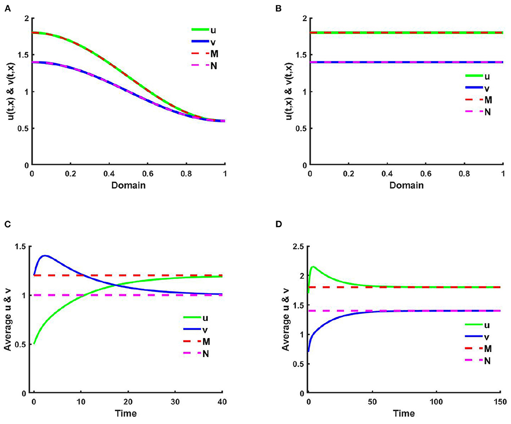
Figure 1. The solutions and space average density of (2.5) when M + N > K where d₁ = d₂ = 1.0, r₁ = r₂ = 1.0 for (A,C) K = 2.0 + cos(π x), M = 0.6K = 1.2 + 0.6 cos(π x), N = 1.0 + 0.4 cos(π x), $\mu (x)=\frac{0.8+0.4cos(\pi x)}{1.5+0.6cos(\pi x)}\in \left[0.66,0.85\right]$, $\nu (x)=\frac{1.0+0.4cos(\pi x)}{0.8+0.4cos(\pi x)}\in \left[0.66,0.88\right]$, (u₀, v₀) = (0.5, 1.2), and (B,D) K = 3.0, M = 0.6K = 1.8, N = 1.5, μ(x) = 0.85, ν(x) = 0.89, (u₀, v₀) = (1.7, 0.7) on Ω = (0, 1).

FIGURE 2

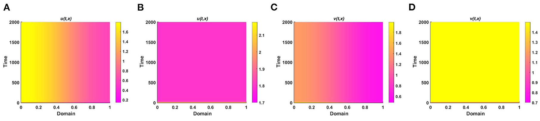
Figure 2. The population density of u and v for (2.5) when M + N > K with d₁ = d₂ = 1.0, r₁ = r₂ = 1.0 for (A,C) K = 2.0 + cos(π x), M = 0.6K = 1.2 + 0.6 cos(π x), N = 1.0 + 0.4 cos(π x), $\mu (x)=\frac{0.8+0.4cos(\pi x)}{1.5+0.6cos(\pi x)}\in \left[0.66,0.85\right]$, $\nu (x)=\frac{1.0+0.4cos(\pi x)}{0.8+0.4cos(\pi x)}\in \left[0.66,0.88\right]$, (u₀, v₀) = (0.5, 1.2), and (B,D) K = 3.0, M = 0.6K = 1.8, N = 1.5, μ(x) = 0.85, ν(x) = 0.89, (u₀, v₀) = (1.7, 0.7) on Ω = (0, 1).

Since μ(x) ∈ [0.66, 0.85] and ν(x) ∈ [0.66, 0.88] in Figures 1A,C, due to the nearly higher impact of ν(x) on v the density of u is found higher than v. Which is also found analogous in Figures 1B,D where K is constant and μ(x) = 0.85, ν(x) = 0.89. It is likewise noted that when K, M, and N are space dependent spatial functions then space average density converges faster to the steady state compared to letting constant values of K, M, and N. It is also observed that density profiles correlate with their corresponding resource functions in all cases, independent of non-negative, non-trivial initial values.

Figure 2 reveals the solution of (2.5) for u and v when t = 2,000. Similar to Figure 1 an attractive coexistence equilibrium solution is noticed for different values of μ and ν.

However, Figure 3 illustrates the solution trajectories for space average density of u vs. v for different initial values (u₀, v₀) when M + N > K, wherein (a) K(x) = 2.0 + cos(π x), M(x) = 0.6K, N(x) = 1.0 + 0.4 cos(π x), $\mu (x)=\frac{0.8+0.4cos(\pi x)}{1.5+0.6cos(\pi x)}\in \left[0.66,0.85\right]$, $\nu (x)=\frac{1.0+0.4cos(\pi x)}{0.8+0.4cos(\pi x)}\in \left[0.66,0.88\right]$ and in (b) K = 3.0, M = 0.6K, and N = 1.5, μ(x) = 0.85, ν(x) = 0.89, for allowing others parameters are fixed. We found that for different constant and non-constant values of competition coefficients both species survive in the competition which is independent of initial values (u₀, v₀).

FIGURE 3

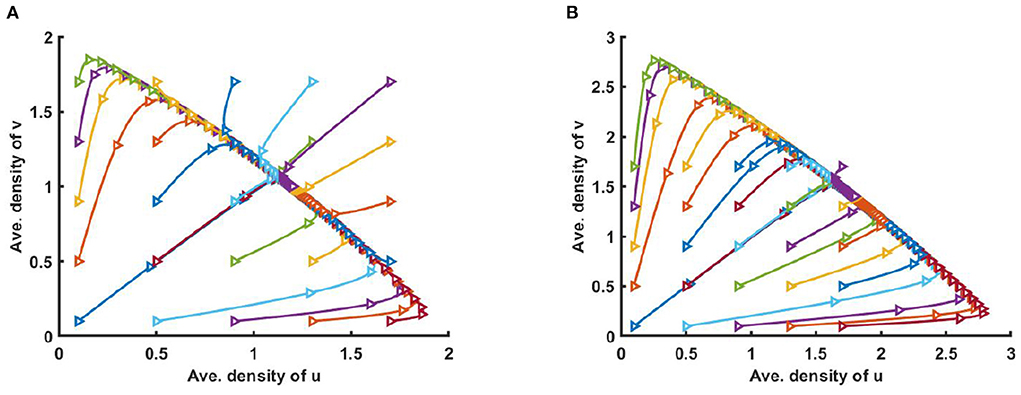
Figure 3. Solution trajectories of space average density of u and v for different initial values (u₀, v₀) on Ω = (0, 1) when M + N > K where d₁ = d₂ = 1.0, r₁ = r₂ = 1.0 for (A) K = 2.0 + cos(π x), M = 0.6K = 1.2 + 0.6 cos(π x), N = 1.0 + 0.4 cos(π x), $\mu (x)=\frac{0.8+0.4cos(\pi x)}{1.5+0.6cos(\pi x)}\in \left[0.85,0.66\right]$, $\nu (x)=\frac{1.0+0.4cos(\pi x)}{0.8+0.4cos(\pi x)}\in \left[0.66,0.88\right]$, and (B) K = 3.0, M = 0.6K = 1.8, N = 1.5, μ(x) = 0.85, ν(x) = 0.89 of (2.5) at t = T = 100.

Example 2. Consider (2.5) when M + N < K for the functions K(x) = 2.0 + cos(π x), where d₁ = d₂ = 1.0, r₁ = r₂ = 1.0, (u₀, v₀) = (0.7, 0.7). Here, setting in Figure 4A M = 0.3K, where N = 1.0 + 0.7 cos(π x), $\mu (x)=\frac{1.4+0.7cos(\pi x)}{1.0+0.7cos(\pi x)}\in \left[1.23,2.33\right]$, $\nu (x)=\frac{1.0+0.3cos(\pi x)}{0.6+0.3cos(\pi x)}\in \left[1.44,2.33\right]$, and in Figure 4B M = 0.6K, and N = 0.6 + 0.4 cos(π x), where $\mu (x)=\frac{0.8+0.4cos(\pi x)}{0.6+0.4cos(\pi x)}\in \left[1.2,2\right]$, $\nu (x)=\frac{1.4+0.6cos(\pi x)}{1.2+0.6cos(\pi x)}\in \left[1.11,1.33\right]$ on Ω = (0, 1). According to Theorem 3, all the solutions either converge to the equilibrium (K(x), 0) or to the equilibrium (0, v^*(x)) which is locally asymptotically stable. Figures 4A,B represents the population density profiles of u and v vs. x for different values of competition coefficients (μ(x), ν(x)) at t = T = 2,000 where the solution is sufficiently large to reach the steady state. Here in all cases, we discover the existence of a competitive exclusion solution. However, in Figure 4A, we observe for small values of proportionality constant (β = 0.3) the species u is endure while v goes to extinction as time raises and the solution of u converges to K with the increase of time. An opposite observation is noticed in Figure 4B where β = 0.6 and the non-trivial solution is found for v, and u turns to elimination for different values of competition coefficients.

FIGURE 4

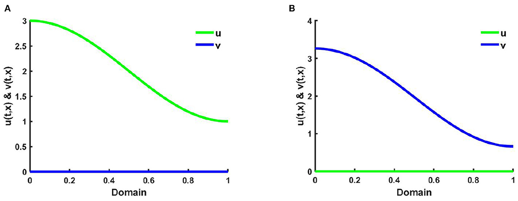
Figure 4. The solutions of (2.5) when M + N < K where K = 2.0 + cos(π x), d₁ = d₂ = 1.0, r₁ = r₂ = 1.0, (u₀, v₀) = (0.7, 0.7) for (A) M = 0.3K = 0.6 + 0.3 cos(π x), N = 1.0 + 0.7 cos(π x), $\mu (x)=\frac{1.4+0.7cos(\pi x)}{1.0+0.7cos(\pi x)}\in \left[1.23,2.33\right]$, $\nu (x)=\frac{1.0+0.3cos(\pi x)}{0.6+0.3cos(\pi x)}\in \left[1.44,2.33\right]$, and (B) M = 0.6K = 1.2 + 0.6 cos(π x), N = 0.6 + 0.4 cos(π x), $\mu (x)=\frac{0.8+0.4cos(\pi x)}{0.6+0.4cos(\pi x)}\in \left[1.2,2\right]$, $\nu (x)=\frac{1.4+0.6cos(\pi x)}{1.2+0.6cos(\pi x)}\in \left[1.11,1.33\right]$ on Ω = (0, 1).

Furthermore, Figure 5 shows the solution trajectories for space average density of u vs. v for different initial values when M + N < K and μ(x), ν(x) > 1. Also let, M = 0.3K, where N = 1.0 + 0.7 cos(π x) in Figure 5A, and M = 0.6K where N = 0.6 + 0.4 cos(π x) in Figure 5B. If M is proportional to K, N/K are non-constant, and M + N < K then by Theorem 3, both semi-trivial equilibrium solutions are locally asymptotically stable. We find that for different non-constant values of competition coefficients one of the species survives in competition, and the solution trajectory moves either toward u or to v depending on the different values of initial values (u₀, v₀).

FIGURE 5

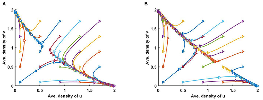
Figure 5. Solution trajectories of space average density of u and v for different initial values (u₀, v₀) on Ω = (0, 1) when M + N < K where K = 2.0 + cos(π x), d₁ = d₂ = 1.0, r₁ = r₂ = 1.0 for (A) M = 0.3K = 0.6 + 0.3 cos(π x), N = 1.0 + 0.7 cos(π x), $\mu (x)=\frac{1.4+0.7cos(\pi x)}{1.0+0.7cos(\pi x)}\in \left[1.23,2.33\right]$, $\nu (x)=\frac{1.0+0.3cos(\pi x)}{0.6+0.3cos(\pi x)}\in \left[1.44,2.33\right]$, and (B) M = 0.6K = 1.2 + 0.6 cos(π x), N = 0.6 + 0.4 cos(π x), $\mu (x)=\frac{0.8+0.4cos(\pi x)}{0.6+0.4cos(\pi x)}\in \left[1.2,2\right]$, $\nu (x)=\frac{1.4+0.6cos(\pi x)}{1.2+0.6cos(\pi x)}\in \left[1.11,1.33\right]$ of (2.5) at t = T = 100.

Example 3. Consider (2.5) where M + N > K and both species disperse according to their resource function M = 1.2 + 0.5 cos(π x) and N = 1.3 + 0.5 cos(π x), respectively which are not proportional to K = 2.0 + cos(π x) in Figures 6, 7, respectively. Also let, d₁ = d₂ = 1.0, r₁ = r₂ = 1.0, (u₀, v₀) = (0.5, 1.2) on Ω = (0, 1) where $\mu (x)=\frac{0.8+0.5cos(\pi x)}{1.3+0.5cos(\pi x)}\in \left[0.37,0.72\right]$, $\nu (x)=\frac{0.7+0.5cos(\pi x)}{1.2+0.5cos(\pi x)}\in \left[0.29,0.70\right]$. In Figure 6, it is observed that the solution approaches the ideal pair (M, N) which is regardless of (u₀, v₀), which is an affirmation of Theorem 4.

FIGURE 6

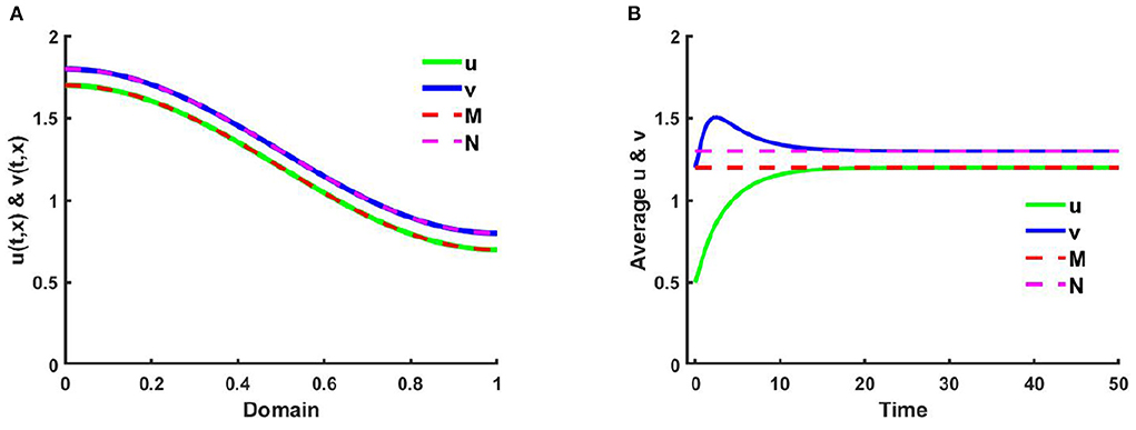
Figure 6. (A) The solutions, and (B) space average density of (2.5) when M + N > K where K = 2.0 + cos(π x), M = 1.2 + 0.5 cos(π x), N = 1.3 + 0.5 cos(π x), $\mu (x)=\frac{0.8+0.5cos(\pi x)}{1.3+0.5cos(\pi x)}\in \left[0.37,0.72\right]$, $\nu (x)=\frac{0.7+0.5cos(\pi x)}{1.2+0.5cos(\pi x)}\in \left[0.29,0.70\right]$, d₁ = d₂ = 1.0, r₁ = r₂ = 1.0, (u₀, v₀) = (0.5, 1.2) on Ω = (0, 1) at t = T = 50.

FIGURE 7

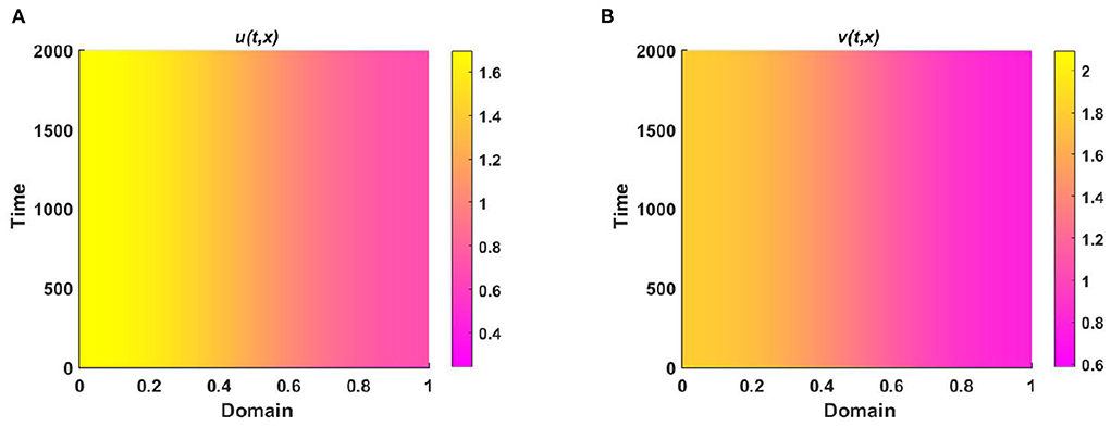
Figure 7. The population density of (A) u, and (B) v for (2.5) when M + N > K where K = 2.0 + cos(π x), M = 1.2 + 0.5 cos(π x), N = 1.3 + 0.5 cos(π x), $\mu (x)=\frac{0.8+0.5cos(\pi x)}{1.3+0.5cos(\pi x)}\in (0.37,0.72)$, $\nu (x)=\frac{0.7+0.5cos(\pi x)}{1.2+0.5cos(\pi x)}\in (0.29,0.70)$, d₁ = d₂ = 1.0, r₁ = r₂ = 1.0, (u₀, v₀) = (0.5, 1.2) on Ω = (0, 1).

Also, Figure 7 illustrates the coexistence of both species is globally asymptotically stable and (u, v) → (M, N) with t → ∞.

5.1.2. Case of two- space dimensions

This section aims to simulate the model (2.5) when K, M, and N are functions of both x and y.

Example 4. Consider the spatial functions for model (2.5) when M + N > K wherein Figures 8A,C K = 2.0 + cos(π x) cos(π y), M = 0.6K = 1.2 + 0.6 cos(π x) cos(π y), N = 1.0 + 0.4 cos(π x) cos(π y), and $\mu (x)=\frac{0.8+0.4cos(\pi x)cos(\pi y)}{1.0+0.4cos(\pi x)cos(\pi y)}\in \left[0.67,0.86\right]$, $\nu (x)=\frac{1.0+0.6cos(\pi x)cos(\pi y)}{1.2+0.6cos(\pi x)cos(\pi y)}\in \left[0.67,0.89\right]$, and in Figures 8B,D K = 3.0, M = 0.6K = 1.8, N = 1.5, μ(x) = 0.8, ν(x) = 0.83. Also let, d₁ = d₂ = 1.0, r₁ = r₂ = 1.0, (u₀, v₀) = (0.7, 0.7) on Ω = (0, 1) × (0, 1) for different values of competition coefficients. Figure 8 signifies the contour profiles of u and v while M is proportional to K and N/K are non-constant. We have computed the solution at t = T = 400 for which it is adequate to get a steady state. We see that for μ(x), ν(x) ∈ (0, 1), both species sustain in the competition, and the contour pattern followed shows a correlation with M and N rather than K. The contour profiles in Figures 8A,C represent the saddle shape where maximum population density is located at the left and right bottom and top corners of the domain whereas minimum population density is found right and left bottom and top corner of the contour profile, respectively. Additionally, also Figures 8B,D shows the coexistence with a very small change in contour profiles. As we know, for two interacting species the outcome is either competitive exclusion or coexistence of two species. Here, we observed that for different constant and space dependent values of μ and ν both species sustain (refer to, Figures 8A–D), which justified Theorem 2 and Corollary 1 while coexistence is feasible. From an ecological perspective, when the competition coefficients are less than 1 then the interspecific competition has less effect than intraspecific competition. The opposite scenario occurs when both competition coefficients are greater than 1. Due to partial resource sharing of both interacting species, competition coefficients (μ, ν) between 0 and 1 stimulate cohabitation in the battle. It is also worth noting that v has a slightly greater population density than u, indicating that species which consume lower per capita accessible resources can have a slightly higher elevated population density. On the other hand, when niche differentiation occurs, most species do not utilize all of the resources available to them. The fish population is one of the most common instances of river organisms. Since one species forages mostly in shallow water and the other in deep water, they can coexist while sharing shared resources. Another example of resource sharing by grazers like zebra and wildebeest which are grazing on plants and eating typical African savanna grass (Panicum maximum) over time. The growing season of this grass begins later in the peak rain and lasts for 6 months. Among the two grazers, zebra eat the tallest grass, which is abundant but less nutritious since zebra teeth allow them to consume the taller grass. Zebras' digestive systems are also more effective than that of a ruminant grazer. However, by eating the tops of the grass, zebra make it simpler for wildebeests to access the more nutrient-dense areas of the grass close to the ground. Despite not being able to digest food as quickly as zebras, wildebeests can gain more energy since the lower portion of the grass is more nutrient-rich and soft. Thus, even though the other animals cannot obtain enough energy from it, they can survive on the shortest grass. In this way, two or more populations can sustain mutually by resource sharing.

FIGURE 8

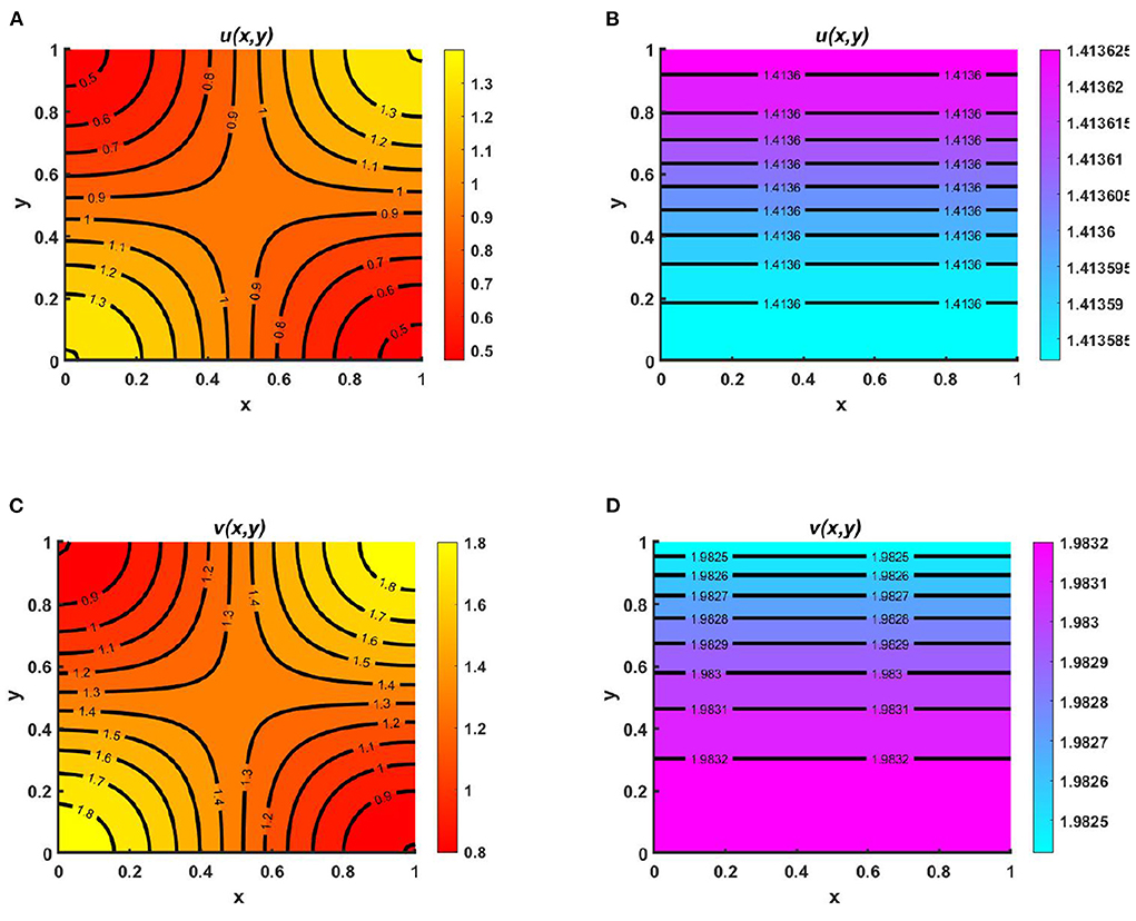
Figure 8. Contour plots of u and v of (2.5) at t = T = 400 when M + N > K where d₁ = d₂ = 1.0, r₁ = r₂ = 1.0, (u₀, v₀) = (0.7, 0.7) for (A,C) K = 2.0 + cos(π x) cos(π y), M = 0.6K = 1.2 + 0.6 cos(π x) cos(π y), N = 1.0 + 0.4 cos(π x) cos(π y), $\mu (x)=\frac{0.8+0.4cos(\pi x)cos(\pi y)}{1.0+0.4cos(\pi x)cos(\pi y)}\in \left[0.67,0.86\right]$, $\nu (x)=\frac{1.0+0.6cos(\pi x)cos(\pi y)}{1.2+0.6cos(\pi x)cos(\pi y)}\in \left[0.67,0.89\right]$, and (B,D) K = 3.0, M = 0.6K = 1.8, N = 1.5, μ(x) = 0.8, ν(x) = 0.83 on Ω = (0, 1) × (0, 1).

Moreover, average scaled density of u, v and u + v of (2.5) are presented in Figure 9 as a function of competition coefficients for M + N > K, where μ ∈ [0.69, 0.9] and ν ∈ [0.65, 0.9] on Ω ∈ (0, 1) × (0, 1) that represents the dependency of the space average population density for μ and ν. Here, we have considered, K = 2.0 + cos(π x) cos(π y), M = 0.6K = 1.2 + 0.6 cos(π x) cos(π y), N = 1.0 + 0.4 cos(π x) cos(π y) while others parameters are fixed as before. We have computed the values of μ(x) and ν(x) at each point in the domain for the range μ ∈ [0.69, 0.9] and ν ∈ [0.65, 0.9] which we have computed from equation (2.6) by the relation of K, M, N, μ, and ν at t = T = 1,000. Figure 9 demonstrates the coexistence of both species for the limited range of μ and ν. At this point, it is mentioned that with the increase of ν, the average density of u rise, whereas it starts to reduce with the increase of μ values. The opposite scenario is noticed for the scaled average population density of v.

FIGURE 9

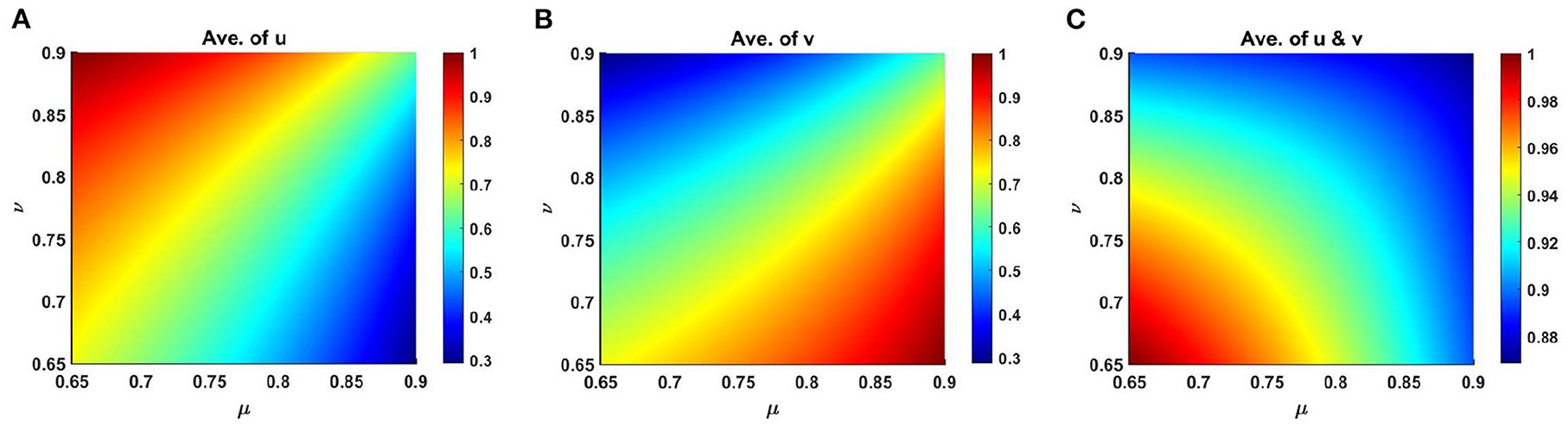
Figure 9. Average scaled density of (2.5) as a function of competition coefficients μ ∈ [0.65, 0.9] and ν ∈ [0.65, 0.9] on Ω ∈ (0, 1) × (0, 1) when M + N > K where d₁ = d₂ = 1.0, r₁ = r₂ = 1.0, (u₀, v₀) = (0.7, 0.7) with K = 2.0 + cos(π x) cos(π y), M = 0.6K = 1.2 + 0.6 cos(π x) cos(π y), N = 1.0 + 0.4 cos(π x) cos(π y) on Ω = (0, 1) × (0, 1) for (A) u, (B) v, and (C) u + v at t = T = 1,000.

Example 5. Consider the case of (2.5) at t = T = 400 when M + N < K where K = 2.0 + cos(π x) cos(π y), d₁ = d₂ = 1.0, r₁ = r₂ = 1.0, (u₀, v₀) = (0.7, 0.7) on Ω = (0, 1) × (0, 1). Here Figures 10A,C characterizes the contour profiles of u and v where we assume M = 0.3K = 0.6 + 0.3 cos(π x) cos(π y), N = 1.0 + 0.7 cos(π x) cos(π y) so that $\mu (x,y)=\frac{1.4+0.7cos(\pi x)cos(\pi y)}{1.0+0.7cos(\pi x)cos(\pi y)}\in \left[1.24,2.33\right]$, $\nu (x,y)=\frac{1.0+0.3cos(\pi x)cos(\pi y)}{0.6+0.3cos(\pi x)cos(\pi y)}\in \left[1.45,2.33\right]$ and in Figures 10B,D M = 0.6K = 1.2 + 0.6 cos(π x) cos(π y), N = 0.6 + 0.4 cos(π x) cos(π y) for which $\mu (x,y)=\frac{0.8+0.4cos(\pi x)cos(\pi y)}{0.6+0.4cos(\pi x)cos(\pi y)}\in \left[1.2,2.0\right]$, $\nu (x,y)=\frac{1.4+0.6cos(\pi x)cos(\pi y)}{1.2+0.6cos(\pi x)cos(\pi y)}\in \left[1.11,1.33\right]$. Here in both cases, competitive exclusion is observed to happen. Depending on the values of proportionally constant β either (u^*, 0) or (0, v^*) that ensure to is attained, which ensures the existence of local semi-trivial equilibrium where the diffusive migration of u followed carrying capacity K and the movement of other species is directed toward their resource distribution N. According to Theorem 3, as time increases, v dies out and the solution of u converges to K as shown in Figures 10A,C. However, in Figures 10B,D, the solution converges to v, and as time grows, u does not sustain in battle. In this case, the values of both competition coefficients are greater than 1, and interspecific competition is strong between the competing species. As we know, one possible effect of intense interspecific competition is competitive exclusion. If two species compete for a similar habitat, then one of them will eventually outcompete the others and drive them out of the environment. On the other hand, due to quite small per capita resource consumption the growth of species u increases rapidly seen in the case of Figures 10A,C, and other populations move toward extinction. A similar observation is noticed in Figures 10B,D for which v sustains in competition. For example, consider bird populations, as most birds rely on the same resources to survive in competition. It could result in fierce rivalry among the species. The more competition in the environment, the more difficult it is to sustain.

FIGURE 10

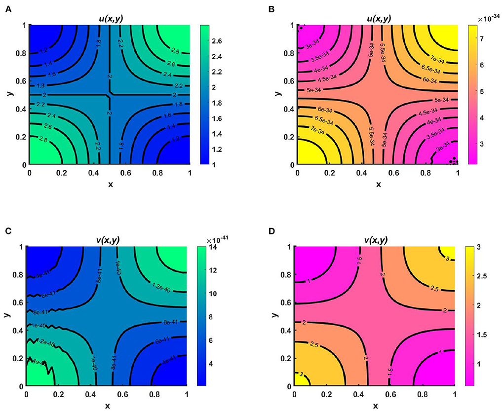
Figure 10. Contour plots of u and v of (2.5) at t = T = 400 when M + N < K where K = 2.0 + cos(π x) cos(π y), d₁ = d₂ = 1.0, r₁ = r₂ = 1.0, (u₀, v₀) = (0.7, 0.7) for (A,C) M = 0.3K = 0.6 + 0.3 cos(π x) cos(π y), N = 1.0 + 0.7 cos(π x) cos(π y), $\mu (x,y)=\frac{1.4+0.7cos(\pi x)cos(\pi y)}{1.0+0.7cos(\pi x)cos(\pi y)}\in \left[1.24,2.33\right]$, $\nu (x,y)=\frac{1.0+0.3cos(\pi x)cos(\pi y)}{0.6+0.3cos(\pi x)cos(\pi y)}\in \left[1.45,2.33\right]$, and (B,D) M = 0.6K = 1.2 + 0.6 cos(π x) cos(π y), N = 0.6 + 0.4 cos(π x) cos(π y), $\mu (x,y)=\frac{0.8+0.4cos(\pi x)cos(\pi y)}{0.6+0.4cos(\pi x)cos(\pi y)}\in \left[1.2,2.0\right]$, $\nu (x,y)=\frac{1.4+0.6cos(\pi x)cos(\pi y)}{1.2+0.6cos(\pi x)cos(\pi y)}\in \left[1.11,1.33\right]$ on Ω = (0, 1) × (0, 1).

However, Figure 11 represents the diagram of scaled average population density of u and v for different levels of competition coefficients at t = T = 1,000. Here μ ∈ [1, 2.5] and ν ∈ [1, 2.5] which is obtained from equation (2.6) on Ω ∈ (0, 1) × (0, 1) for M + N < K when M = 0.3K and N = 1.0 + 0.7 cos(π x) cos(π y). Here, we have calculated the dependency of u and v at each point for the consider fixed upper and lower estimates of μ and ν in the domain.

FIGURE 11

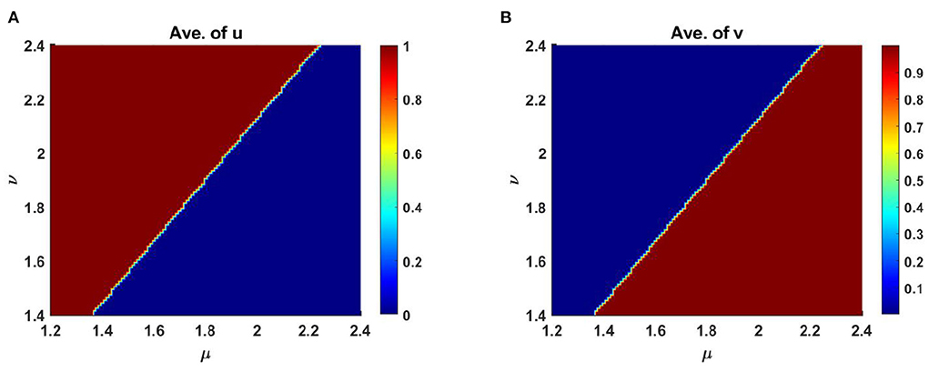
Figure 11. Average scaled density of u and v of (2.5) as a function of competition coefficients μ ∈ [1, 2.5] and ν ∈ [1, 2.5] on Ω ∈ (0, 1) × (0, 1) when M + N > K with K = 2.0 + cos(π x) cos(π y), M = 0.3K = 0.6 + 0.3 cos(π x) cos(π y), N = 1.0 + 0.7 cos(π x) cos(π y), d₁ = d₂ = 1.0, r₁ = r₂ = 1.0, (u₀, v₀) = (0.7, 0.7) on Ω = (0, 1) × (0, 1) at t = T = 1,000.

Also, Figure 12 reveals the comparison of the average scaled population density of u and v for different levels of competition coefficients where μ ∈ [1, 2] and ν ∈ [1, 2] on Ω ∈ (0, 1) × (0, 1) at time t = T = 1,000. Here we set, M = 0.6K = 1.2 + 0.6 cos(π x) cos(π y), N = 0.6 + 0.4 cos(π x) cos(π y) and considering other parameters are fixed as before.

FIGURE 12

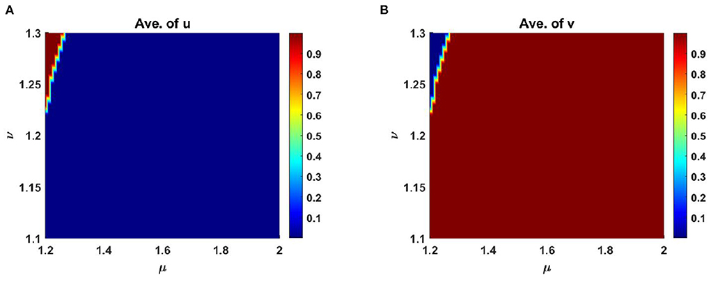
Figure 12. Average scaled density of u and v of (2.5) as a function of competition coefficients μ ∈ [1.2, 2] and ν ∈ [1.1, 1.3] on Ω ∈ (0, 1) × (0, 1) when M + N > K with K = 2.0 + cos(π x) cos(π y), M = 0.6K = 1.2 + 0.6 cos(π x) cos(π y), N = 0.6 + 0.4 cos(π x) cos(π y), d₁ = d₂ = 1.0, r₁ = r₂ = 1.0, (u₀, v₀) = (0.7, 0.7) on Ω = (0, 1) × (0, 1) at t = T = 1,000.

Example 6. Take K = 2.0 + cos(π x) cos(π y) where M = 0.9 + 0.5 cos(π x) cos(π y), N = 1.1 + 0.5 cos(π x) cos(π y) in Figures 13A,B and M = 1.5 + 0.6 cos(π x) cos(π y), N = 0.8 + 0.7 cos(π x) cos(π y) in Figures 13C,D on Ω = (0, 1) × (0, 1) for the model (2.5) when M + N ≥ K for which the contour profiles in Figure 13 form an ideal free pair. Here also let, d₁ = d₂ = 1.0, r₁ = r₂ = 1.0, (u₀, v₀) = (0.5, 0.5) where μ(x, y) = ν(x, y) = 1.0 and $\mu (x,y)=\frac{0.5+0.4cos(\pi x)cos(\pi y)}{0.8+0.7cos(\pi x)cos(\pi y)}\in \left[0.6,1.0\right]$, $\nu (x,y)=\frac{1.2+0.3cos(\pi x)cos(\pi y)}{1.5+0.6cos(\pi x)}\in \left[0.71,1.0\right]$, respectively in the prescribed domain. Here, we perceive that the contour profile of u follows M and the contour profiles of v correlate with N, respectively (refer to, Figures 13A,B) while M + N = K. In this case both species are diffusing in the direction of their resource functions and for the fixed values of competition coefficients, the coexistence of species appears, and they form an ideal pair. The total density for such a pair is identical to the carrying capacity. In this condition, the availability of resources for the couple species is spatially distinct, which can specialize through resource consumption. However, a similar observation is noticed for the case M + N > K (refer to, Figures 13C,D) and the contour profile approaches toward their respective resource function that will form an ideal pair with the increase of time, which is one of the confirmations of the Theorem 4.

FIGURE 13

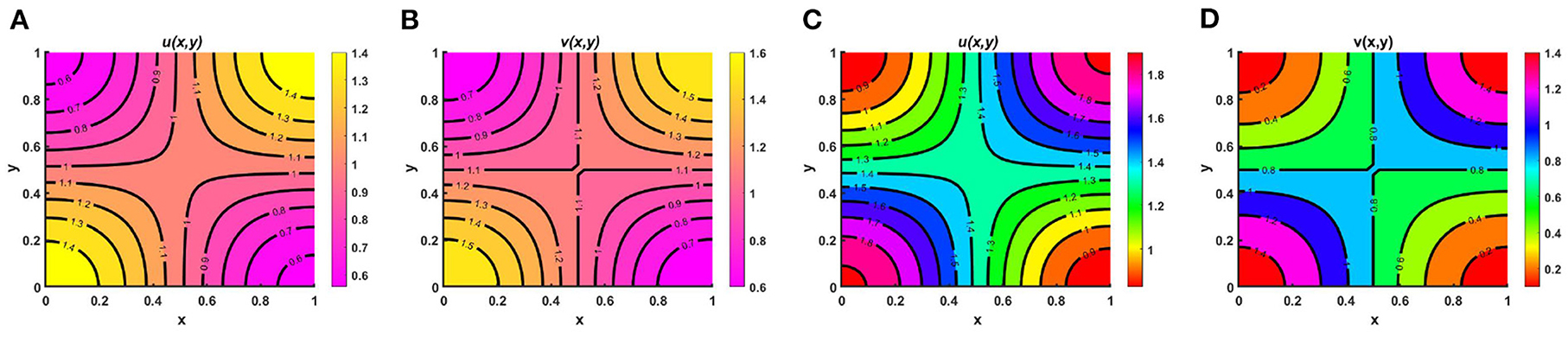
Figure 13. Contour plots of u and v of (2.5) at t = T = 350 when M + N ≥ K with K = 2.0 + cos(π x) cos(π y) for (A,B) M = 0.9 + 0.5 cos(π x) cos(π y), N = 1.1 + 0.5 cos(π x) cos(π y), μ(x, y) = 1.0, ν(x, y) = 1.0, and (C,D) M = 1.5 + 0.6 cos(π x) cos(π y), N = 0.8 + 0.7 cos(π x) cos(π y), $\mu (x,y)=\frac{0.5+0.4cos(\pi x)cos(\pi y)}{0.8+0.7cos(\pi x)cos(\pi y)}\in \left[0.6,1.0\right]$, $\nu (x,y)=\frac{1.2+0.3cos(\pi x)cos(\pi y)}{1.5+0.6cos(\pi x)}\in \left[0.71,1.0\right]$, d₁ = d₂ = 1.0, r₁ = r₂ = 1.0, (u₀, v₀) = (0.5, 0.5) on Ω = (0, 1) × (0, 1).

5.2. When K, M, N, μ, and ν are time dependent

5.2.1. Case of two-space dimensions

In this section, we will study the model (2.5) numerically when K, M, and N are two-dimensional time dependent functions, which may occur for seasonal variations. We will present the instantaneous contour profiles of u(t, x, y) and v(t, x, y) for t = T, $t=T+\frac{2\pi }{k\Omega }$ where k = 1, 2, …, that confirm the existence of a positive periodic state during a particular time interval. Here, T is substantially sufficient to reach the time periodicity of the population density. Furthermore, we exhibit the space averaged density profile as a function of time to show its approach to a periodic state. Here we will compare the time periodic case with the case of steady state only by including the time periodic function. The time dependent case has been computed to examine, do the periodic state represents the same patterns as the same steady state cases studied in the earlier section? We will discover this question in this section.

Example 7. Consider the time dependent functions for the case of (2.5) when M + N > K where K = (2.0 + cos(π x) cos(π y))(1.0 + 0.2 cos(t)), M = 0.6K = (1.2 + 0.6 cos(π x) cos(π y))(1.0 + 0.2 cos(t)), N = (1.0 + 0.4 cos(π x) cos(π y))(1.0 + 0.2 cos(t)) on Ω = (0, 1) × (0, 1). Here μ(t, x, y) ∈ [0.67, 0.86], ν(t, x, y) ∈ [0.67, 0.89] with r₁ = r₂ = r = 1.0, (u₀, v₀) = (0.5, 0.5), d₁ = d₂ = 1.0. Here, Figure 14 demonstrates the instantaneous change in population development of u(t, x, y) and v(t, x, y) through contour profiles for a specific time period. At this point, we have computed the instantaneous contour profiles of u for (Figure 14A) T, (Figure 14B) $T+\frac{\pi }{2}$, (Figure 14C) T + π, (Figure 14D) $T+\frac{3\pi }{2}$, and (Figure 14E) T + 2π, where t = T = 38.55, which is large enough to reach the steady state. As we know, due to seasonal variation or any other periodic factors during a time phase, the population growth is not always even everywhere, its growth rises and falls during specific seasons. There are many reasons, such as food availability, space, water supply, climate change, diseases, and predators that influence the growth of population during a time interval.

FIGURE 14

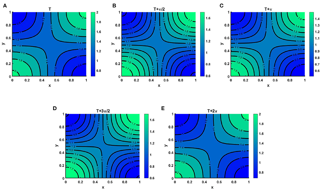
Figure 14. Contour plots of u(t, x, y) of (2.5) when M + N > K where K = (2.0 + cos(π x) cos(π y))(1.0 + 0.2 cos(t)), M = 0.6K = (1.2 + 0.6 cos(π x) cos(π y))(1.0 + 0.2 cos(t)), N = (1.0 + 0.4 cos(π x) cos(π y))(1.0 + 0.2 cos(t)), μ(t, x, y) ∈ [0.67, 0.86], ν(t, x, y) ∈ [0.67, 0.89], r₁ = r₂ = r = 1.0, (u₀, v₀) = (0.5, 0.5), d₁ = d₂ = 1.0, Ω = (0, 1) × (0, 1) for (A) T, (B) $T+\frac{\pi }{2}$, (C) T + π, (D) $T+\frac{3\pi }{2}$, and (E) T + 2π, where T = 38.55.

Thus, at all times during a period, we will not get the same population density. As we have shown in Figure 14. We observe that at T = 38.55 and T = 38.55 + 2π the instantaneous contours plots correspond to identical values that provide the existence of positive periodic solutions. It is also noted that Figure 14 corresponds to Figure 8A of the steady state case for which both species survive in competition. Here, we have only included the time periodic function with the same steady state function to see the existence of the periodic state.

However, Figure 15 represents the instantaneous contour profiles of v(t, x, y) for (Figure 15A) T, (Figure 15B) $T+\frac{\pi }{2}$, (Figure 15C) T + π, (Figure 15D) $T+\frac{3\pi }{2}$, and (Figure 15E) T + 2π, where t = T = 19.71 for which species v is found to survive. Similar to Figure 14, we observe that at T = 19.71 and T = 19.71 + 2π the instantaneous contours plots of v(t, x, y) resemble indistinguishable values which corresponds to Figure 8C of the steady state case.

FIGURE 15

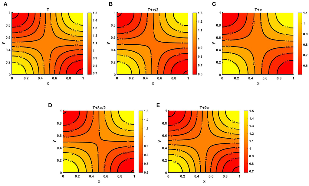
Figure 15. Contour plots of v(t, x, y) of (2.5) when M + N > K where K = (2.0 + cos(π x) cos(π y))(1.0 + 0.2 cos(t)), M = 0.6K = (1.2 + 0.6 cos(π x) cos(π y))(1.0 + 0.2 cos(t)), N = (1.0 + 0.4 cos(π x) cos(π y))(1.0 + 0.2 cos(t)), μ(t, x, y) ∈ [0.67, 0.86], ν(t, x, y) ∈ [0.67, 0.89], r₁ = r₂ = r = 1.0, (u₀, v₀) = (0.5, 0.5), d₁ = d₂ = 1.0, Ω = (0, 1) × (0, 1) for (A) T, (B) $T+\frac{\pi }{2}$, (C) T + π, (D) $T+\frac{3\pi }{2}$, and (E) T + 2π, where T = 19.71.

Example 8. Consider K = (2.0 + cos(π x) cos(π y))(1.0 + 0.2 cos(t)) when M + N < K where M = 0.3K = (0.6 + 0.3 cos(π x) cos(π y))(1.0 + 0.2 cos(t)), N = (1.0 + 0.7 cos(π x) cos(π y))(1.0 + 0.2 cos(t)), μ(t, x, y) ∈ [1.23, 2.33], ν(t, x, y) ∈ [1.44, 2.33] in Figures 16A,B and M = 0.6K = (1.2 + 0.0.6 cos(π x) cos(π y))(0.6 + 0.4 cos(t)), N = (0.6 + 0.4 cos(π x) cos(π y))(1.0 + 0.2 cos(t)), μ(t, x, y) ∈ [1.2, 2.0], ν(t, x, y) ∈ [1.11, 1.33] in Figures 16C,D. Also let, r₁ = r₂ = r = 1.0, (u₀, v₀) = (0.5, 0.5), d₁ = d₂ = 1.0 on Ω = (0, 1) × (0, 1). The time average over a specific time interval are $\langle u(.,x,y)\rangle =\frac{1}{2\pi }\underset{T}{\overset{2\pi +T}{\int }}u(t,x,y)dt$ and $\langle v(.,x,y)\rangle =\frac{1}{2\pi }\underset{T}{\overset{2\pi +T}{\int }}v(t,x,y)dt$, respectively. It is noticed that the time average profiles in Figures 16A,B is similar to the steady pattern in Figures 10A,C. We found that due to intense interspecific competition and slightly higher values of ν compared to μ species u is persist and v dies out (refer to, Figures 16A,B), which is expected according to Theorem 3. Also, the contour profile of u corresponds to the contour pattern of K with the increase of time. Opposite observation is found while considering M = 0.6K, and N = (0.6 + 0.4 cos(π x) cos(π y))(1.0 + 0.2 cos(t)) for μ, ν > 1 and it is observed that the time average for periodic time dependent function the patterns in Figures 16C,D correspond to the steady state patterns in Figures 10B,D.

FIGURE 16

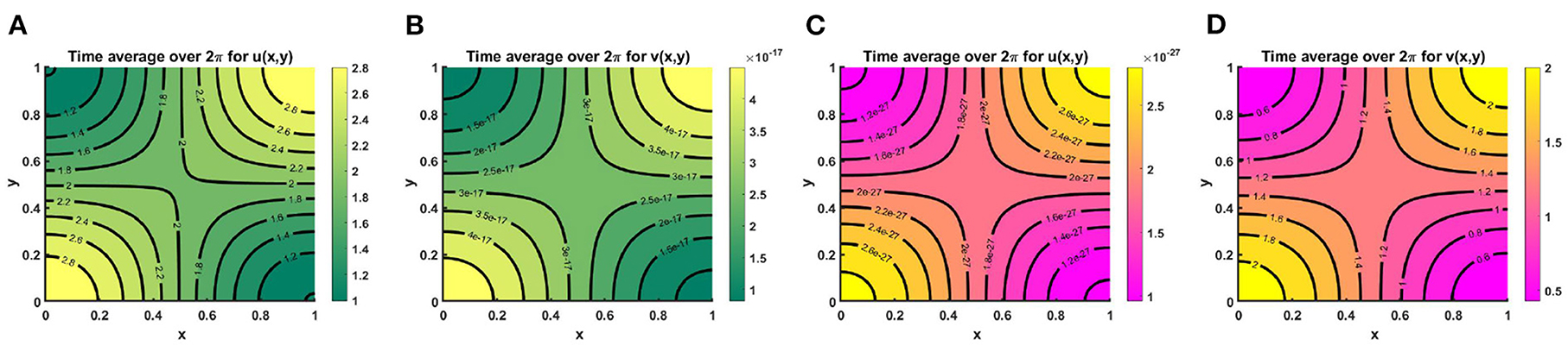
Figure 16. Contour plots of 〈u(., x, y)〉, and 〈v(., x, y)〉 of (2.5) when M + N < K where K = (2.0 + cos(π x) cos(π y))(1.0 + 0.2 cos(t)), r₁ = r₂ = r = 1.0, (u₀, v₀) = (0.5, 0.5), d₁ = d₂ = 1.0, for (A,B) M = 0.3K = (0.6 + 0.3 cos(π x) cos(π y))(1.0 + 0.2 cos(t)), N = (1.0 + 0.7 cos(π x) cos(π y))(1.0 + 0.2 cos(t)), μ(t, x, y) ∈ [1.23, 2.33], ν(t, x, y) ∈ [1.44, 2.33], and (C,D) M = 0.6K = (1.2 + 0.0.6 cos(π x) cos(π y))(0.6 + 0.4 cos(t)), N = (0.6 + 0.4 cos(π x) cos(π y))(1.0 + 0.2 cos(t)), μ(t, x, y) ∈ [1.2, 2.0], ν(t, x, y) ∈ [1.11, 1.33] on Ω = (0, 1) × (0, 1).

Example 9. Consider the time dependent function for model (2.5) when M + N ≥ K on Ω = (0, 1) × (0, 1). Assume K = (2.0 + cos(π x) cos(π y))(1.0 + 0.2 cos(t)), M = (1.5 + 0.0.6 cos(π x) cos(π y))(1.0 + 0.2 cos(t)), N = (0.8 + 0.7 cos(π x) cos(π y))(1.0 + 0.2 cos(t)) for which μ(t, x, y) ∈ [0.6, 1.0], ν(t, x, y) ∈ [0.71, 1.0]. Also let, r₁ = r₂ = r = 1.0, (u₀, v₀) = (0.5, 0.5), d₁ = d₂ = 1.0. We get the time average contour profiles of u(t, x, y) and v(t, x, y) produce ideal pair for the time dependent function which converges to M and N as time grows up. Also, the time average contour profiles in Figure 17 relate to the steady state pattern in Figure 13. We find that while both M and N are non-proportional with K than for μ, ν ∈ (0, 1) both species survive and pick up the finest solution (M, N) known as the ideal free pair.

FIGURE 17

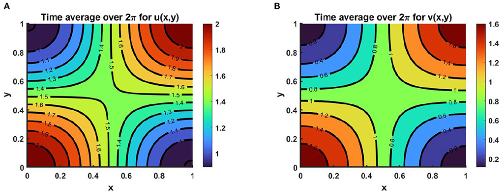
Figure 17. Contour plots of 〈u(., x, y)〉, and 〈v(., x, y)〉 of (2.5) when M + N ≥ K where K = (2.0 + cos(π x) cos(π y))(1.0 + 0.2 cos(t)), M = (1.5 + 0.0.6 cos(π x) cos(π y))(1.0 + 0.2 cos(t)), N = (0.8 + 0.7 cos(π x) cos(π y))(1.0 + 0.2 cos(t)), μ(t, x, y) ∈ [0.6, 1.0], ν(t, x, y) ∈ [0.71, 1.0], r₁ = r₂ = r = 1.0, (u₀, v₀) = (0.5, 0.5), d₁ = d₂ = 1.0 on Ω = (0, 1) × (0, 1).

6. Summary of the study

We studied two species' competition dynamics that describe the competition and cooperation of both species in a heterogeneous environment with different imposed diffusion strategies. Several results have been established, considering the weak and strong competition, based on the intensity of spatially dependent competition coefficients. For a generalized non-symmetric growth function, we have discovered that if the first species follow K− driven diffusion and at the same time, the other species diffuse according to their resource distribution, then in the case of weak competition (μ(x), ν(x) < 1) both species sustain in the competition. Additionally, rising over time, its solution converges to the resource functions, forming an ideal free pair. However, in the case of strong competition (μ(x), ν(x) > 1), no coexistence is possible and there exists at least one semi-trivial solution. Furthermore, if both organisms follow the resource base diffusion, then once again, for μ(x), ν(x) < 1 ideal pair is guaranteed to be attained in battle. The model's efficacy for the case of one and two space dimensions is presented via numerical computation both for space and time-dependent cases, which is very effective from an ecological perspective. The findings may provide insight into the management of species invasions. If a more efficient diffuser is an invader, and all other factors remain constant, the invasive species' higher competitive coefficient may drive the local species to extinction. In addition, the enforced diffusion tactics are essential for researching grazing animals, marine organisms, and various winter birds. On the other hand, the population always moves in a good environment and leaves an unfavorable one, which can lead to unpredictable habits, like human behavior. The idea of different diffusion strategies is often closely connected to the creation and diffusion of knowledge as well as to the technological evolution of society. For more current advanced study on the model of human dynamical analysis, refer to Ali et al. [24]. The outcomes of the investigation can be extended by considering three species' population dynamics while they follow similar diffusion strategies with different competition coefficients.

Data availability statement

The original contributions presented in the study are included in the article/supplementary material, further inquiries can be directed to the corresponding authors.

Author contributions

IZ and MK: conceptualization, formal analysis, software, and original draft preparation. IZ, MK, and MA: methodology. MM and TK: validation and investigation. TK and MA: resources. IZ: data curation. MA, MM, and TK: review and editing. MK: supervision. All the authors have read and agreed to the published version of the manuscript.

Funding

The authors acknowledged the reviewers for their comments and suggestions which significantly improve the quality of the manuscript. The author MM, research was supported by National Science Foundation grant DMS-2213274, and University Research grant, TAMIU. Also, the author, MK's research, was partially supported by the Ministry of Science and Technology (MOST), EAS 488 for the year 2021-2022, Bangladesh.

Conflict of interest

The authors declare that the research was conducted in the absence of any commercial or financial relationships that could be construed as a potential conflict of interest.

Publisher's note

All claims expressed in this article are solely those of the authors and do not necessarily represent those of their affiliated organizations, or those of the publisher, the editors and the reviewers. Any product that may be evaluated in this article, or claim that may be made by its manufacturer, is not guaranteed or endorsed by the publisher.

References

1. Averill I, Lou Y, Munther D. On several conjectures from evolution of dispersal. J Biol Dyn. (2012) 6:117–30. doi: 10.1080/17513758.2010.529169

PubMed Abstract | CrossRef Full Text | Google Scholar

2. Chen X, Lam KY, Lou Y. Dynamics of a reaction-diffusion-advection model for two competing species. Discrete Contin Dyn Syst. (2012) 32:3841–59. doi: 10.3934/dcds.2012.32.3841

PubMed Abstract | CrossRef Full Text | Google Scholar

3. Dockery J, Hutson V, Mischaikow K, Pernarowski M. The evolution of slow dispersal rates: a reaction diffusion model. J Math Biol. (1998) 37:61–83. doi: 10.1007/s002850050120

PubMed Abstract | CrossRef Full Text | Google Scholar

4. Braverman E, Braverman L. Optimal harvesting of diffusive models in a nonhomogeneous environment. Nonlinear Anal Theory Meth Appl. (2009) 71:e2173–81. doi: 10.1016/j.na.2009.04.025

CrossRef Full Text | Google Scholar

5. Cantrell RS, Cosner C, Lou Y. Approximating the ideal free distribution via reaction-diffusion-advection equations. J Differ Equat. (2008) 245:3687–707. doi: 10.1016/j.jde.2008.07.024

CrossRef Full Text | Google Scholar

6. Cantrell RS, Cosner C, Lou Y. Evolution of dispersal and the ideal free distribution. Math Biosci Eng. (2010) 7:17–36. doi: 10.3934/mbe.2010.7.17

PubMed Abstract | CrossRef Full Text | Google Scholar

7. Cantrell RS, Cosner C. Spatial Ecology via Reaction-diffusion Equations, Wiley Series in Mathematical and Computational Biology. Chichester: John Wiley & Sons (2003).

Google Scholar

8. Braverman E, Ilmer I. On the interplay of harvesting and various diffusion strategies for spatially heterogeneous population. J Theor Biol. (2019) 466:106–18. doi: 10.1016/j.jtbi.2019.01.024

PubMed Abstract | CrossRef Full Text | Google Scholar

9. Braverman E, Kamrujjaman M. Competitive-cooperative models with various diffusion strategies. Comput Math Appl. (2016) 72:653–62. doi: 10.1016/j.camwa.2016.05.017

CrossRef Full Text | Google Scholar

10. Korobenko L, Braverman E. A logistic model with a carrying capacity driven diffusion. Can Appl Math Quart. (2009) 17:85–104.

PubMed Abstract

11. Kamrujjaman M. Directed vs regular diffusion strategy: evolutionary stability analysis of a competition model and an ideal free pair. Differ Equat Appl. (2019) 11:267–90. doi: 10.7153/dea-2019-11-11

CrossRef Full Text | Google Scholar

12. Kamrujjaman M. Weak competition and ideally distributed population in a cooperative diffusive model with crowding effects. Phy Sci I J. (2018) 18:1–16. doi: 10.9734/PSIJ/2018/42472

CrossRef Full Text | Google Scholar

13. Morita Y, Tachibana K. An entire solution to the Lotka-Volterra competition-diffusion equations. SIAM J Math Anal. (2009) 40:2217–40. doi: 10.1137/080723715

CrossRef Full Text | Google Scholar

14. He X, Ni MW. The effects of diffusion spatial variation in Lotka—Volterra competition–diffusion system I: heterogeneity vs. homogeneity. J Differ Equat. (2013) 254:528–46. doi: 10.1016/j.jde.2012.08.032

CrossRef Full Text | Google Scholar

15. Braverman E, Kamrujjaman M. Lotka systems with directed dispersal dynamics: competition and influence of diffusion strategies. Math Biosci. (2016) 279:1–12. doi: 10.1016/j.mbs.2016.06.007

PubMed Abstract | CrossRef Full Text | Google Scholar

16. Gilpin ME, Ayala FJ. Global models of growth and competition. Proc Natl Acad Sci USA. (1973) 70:3590–3. doi: 10.1073/pnas.70.12.3590

PubMed Abstract | CrossRef Full Text | Google Scholar

17. Gompertz B. On the nature of the function expressive of human mortality and on a a new mode of determining the value of life contingencies. Philo Trans R Soc Lond. (1825) 115:513–83. doi: 10.1098/rstl.1825.0026

PubMed Abstract | CrossRef Full Text | Google Scholar

18. Smith FE. Population dynamics in Daphnia Magna and a new model for population, Ecology. (1963) 44:651–63. doi: 10.2307/1933011

CrossRef Full Text | Google Scholar

19. Wang Q. Some global dynamic of a Lotka-Volterra competition-diffusion-advection system. Commun Pure Appl. Math. (2020) 19:3245–55. doi: 10.3934/cpaa.2020142

CrossRef Full Text | Google Scholar

20. Kot M. Elements of Mathematical Ecology. Cambridge: Cambridge University Press (2001).

Google Scholar

21. Korobenko L, Braverman E. On evolutionary stability of carrying capacity driven dispersal in competition with regularly diffusing populations. J Math Biol. (2014) 69:1181–206. doi: 10.1007/s00285-013-0729-8

PubMed Abstract | CrossRef Full Text | Google Scholar

22. Pao CV. Nonlinear Parabolic and Elliptic Equations. New York, NY: Plenum (1992).

Google Scholar

23. Smith HL. Monotone dynamical systems: an introduction to the theory of competitive and cooperative system. Amer Math Soc. (2008) 33:41. doi: 10.1090/surv/041

CrossRef Full Text | Google Scholar

24. Ali A, Alshammari SF, Islam S, Khan MA, Ullah S. Modeling and analysis of the dynamics of novel coronavirus (COVID-19) with Caputo fractional derivative. Results Phys. (2021) 20:103669. doi: 10.1016/j.rinp.2020.103669

PubMed Abstract | CrossRef Full Text | Google Scholar