A New Tobit Ridge-Type Estimator of the Censored Regression Model With Multicollinearity Problem

Introduction

The limited dependent variables (LDVs) in the regression models are defined as the censored, the discrete, and the truncated outcomes. Tobin [1] introduced the Tobit model of the censored dependent variable, which is related to the LDVs, and Goldberger [2] gave its current name. The censored data appear when the dependent variable has a loss of information, while the truncated data appear when the dependent and the independent variables have a loss of information. In this study, we used the standard Tobit regression model, which is the Type 1 model of the Tobit models (Type 1–5) categorized by Amemiya [3] to deal with the censored dataset and their estimation. The censored normal regression model, which is called the Tobit model, is used to relieve the deficiency of biasedness and inconsistency of the results of using the least squares estimator (LSE). Therefore, to determine the estimates of the parameter and to find the estimates of statistical inference, the Tobit maximum likelihood estimator (TMLE) is used. When the explanatory (independent) variables are not independent, it becomes a problem called multicollinearity, which this problem often ignored in the censored regression models. Also, the multicollinearity makes the Tobit maximum likelihood estimates of the regression coefficients incorrect, unreliable, and unstable; because the mean squared error (MSE) values of these estimates are inflated. For this case, Khalaf et al. [4] examined the multicollinearity effects on the TMLE, and they introduced the Tobit ridge estimator (TRE). Then, Alhusseini and Odah [5] introduced a Tobit principal component estimator. Also, Toker et al. [6] introduced a Tobit Liu estimator (TLE).

In the linear regression model (LRM), several alternative estimators of the regression coefficients have been produced for the LSE when the multicollinearity problem happens because, in this case, the LSE gives large variances, wrong signs, and becomes unstable. The most popular estimators are the ridge estimator of Hoerl and Kennard [7] and the Liu estimator of Liu [8]. Recently, Kibria and Lukman [9] proposed a new ridge-type estimator (NRTE). The NRTE has been extended in different regression models in different studies, such as Lukman et al. [10], Lukman et al. [11], Akram et al. [12], Dawoud and Abonazel [13], Awwad et al. [14], and Abonazel et al. [15]. The multicollinearity is known to be a terrible problem in the Tobit model like in the LRM. For handling multicollinearity, some studies gave and investigated some biased estimators in the LRM for a long time, but there is little investigation of these estimators in the Tobit model. However, studies of the biased estimators instead of TMLE in deleting multicollinearity effects on regression coefficients in the Tobit model are needed. In this context, the TRE was introduced by Khalaf et al. [4] and the TLE by Toker et al. [6] were the biased estimation beginning points in the Tobit model. Then, we defined the Tobit NRTE (TNRTE) in this study. Also, we focus on the theoretical properties of the TNRTE by the MSE criterion and to compare them to the TMLE, the TRE, and the TLE.

The next content of this study is given as follows: Methodology Section defines the Tobit regression model and provides the TNRTE and the theoretical properties. A Monte Carlo Simulation Section deals with the Monte Carlo simulation study. A Real Life Data Section deals with the Mroz dataset. Conclusion Section includes the concluding remarks.

Methodology

Tobit Regression Model

The model of the Tobit regression is

$\begin{array}{ll}{y}_i^{*}=x_i\beta +u_i;i=1,2,...,n,& (1)\end{array}$

where $y_i^{*}$ is called the dependent latent variable, x_i is an i-th row of the known matrix X with the dimension n × (p + 1); where p is the number of the explanatory variables. β is the unknown (p + 1) × 1 coefficient vector (when the model contains the intercept β₀), and u_i is called an error term that is independent, follows a normal distribution by mean, and equals 0 and variance equals σ². We considered the left censoring, where y_i is defined as follows:

$\begin{array}{ll}{y}_i=\{\begin{array}{cc}{y}_i^{*},& if{y}_i^{*}>0\\ 0,& otherwise\end{array}& (2)\end{array}$

On the basis of n observations on y_i and x_i, the β and σ² estimation issues are noted. For the defined model in Equation (1), assuming that n_a is the observation number for y_i = 0 and is the observation number for y_i > 0, that is, non-zero for y_i occur first, then the log-likelihood function of the censored data is given as

$\begin{array}{l}logS(X;\beta ,{\sigma }^2)={\displaystyle \sum _{n_a}}log(1-G_i)+{\displaystyle \sum _{n_b}}log\left(\frac{1}{\sigma \sqrt{2\pi }}\right)\\ -{\displaystyle \sum _{n_b}}\frac{1}{2{\sigma }^2}{(y_i-x_i\beta )}^2,& (3)\end{array}$

where $G_i=\underset{-\infty }{\overset{x_i\beta }{\int }}\frac{1}{\sigma \sqrt{2\pi }}{e}^{-\frac{1}{2{\sigma }^2}{q}^2}dq$.

The TMLE of β is identified after solving the derivate of Equation (3), but it is not a linear function of β, so it can be solved iteratively by Fisher's scoring method that comprises using the second derivative. The Fisher's scoring method is given as

$\begin{array}{ll}{\widehat{\beta }}^{(r)}={\widehat{\beta }}^{(r-1)}-L^{-1}({\widehat{\beta }}^{(r-1)})Q({\widehat{\beta }}^{(r-1)}).r=1,2,...,& (4)\end{array}$

where $L({\widehat{\beta }}^{(r-1)})=E{\left(\frac{{\partial }^{2}logS(X;\beta ,{\sigma }^2)}{\partial \beta \partial {\beta }^{\prime }}\right)}_{\beta ={\widehat{\beta }}^{(r-1)}}=\frac{1}{{\sigma }^2}\stackrel{-}{D}$ is the matrix of the Fisher information which is given at ${\widehat{\beta }}^{(r-1)}$ where ${\widehat{\beta }}^{(r)}$ is β estimate at iteration(r), ${\widehat{\beta }}^{(r-1)}$ is β estimate at iteration (r − 1), $\stackrel{-}{D}=X^{\prime }DX$, D is called as the diagonal matrix and $Q({\widehat{\beta }}^{(r-1)})=E{\left(\frac{\partial logS(X;\beta ,{\sigma }^2)}{\partial \beta }\right)}_{\beta ={\widehat{\beta }}^{(r-1)}}.$ So, the TMLE is written as:

$\begin{array}{l}{\widehat{\beta }}^{(r)}={\widehat{\beta }}^{(r-1)}-{\sigma }^2{(\stackrel{-}{D})}^{-1}Q({\widehat{\beta }}^{(r-1)})\\ ={(\stackrel{-}{D})}^{-1}(\stackrel{-}{D}{\widehat{\beta }}^{(r-1)}-{\sigma }^{2}Q({\widehat{\beta }}^{(r-1)})).& (5)\end{array}$

Then, $Q({\widehat{\beta }}^{(r-1)})$is given as:

$\begin{array}{ll}Q({\widehat{\beta }}^{(r-1)})=\frac{1}{{\sigma }^2}(\stackrel{-}{D})({\widehat{\beta }}^{(r-1)}-{\widehat{\beta }}^{(r)}).& (6)\end{array}$

Since the TMLE becomes inefficient and unstable when the multicollinearity problem occurs, Khalaf et al. [4] proposed the TRE and Toker et al. [6] proposed the TLE to eliminate the effects of this problem.

The TRE is given iteratively as

$\begin{array}{ll}{\widehat{\beta }}_k^{(r)}={\widehat{\beta }}_k^{(r-1)}-{\left[{\widehat{\beta }}^{(r-1)}-{(\stackrel{-}{D}+kI)}^{-1}(\stackrel{-}{D}){\widehat{\beta }}^{(r)}\right]}_{\beta ={\widehat{\beta }}^{(r-1)}}& (7)\end{array}$

and the first step of the TRE is

$\begin{array}{l}{\widehat{\beta }}_k^{(1)}={\widehat{\beta }}_k^{(0)}-{\left[{\widehat{\beta }}^{(0)}-{(\stackrel{-}{D}+kI)}^{-1}(\stackrel{-}{D}){\widehat{\beta }}^{(1)}\right]}_{\beta ={\widehat{\beta }}^{(0)}}\\ ={({\widehat{\stackrel{-}{D}}}^{(0)}+kI)}^{-1}({\widehat{\stackrel{-}{D}}}^{(0)}){\widehat{\beta }}^{(1)},& (8)\end{array}$

such that ${\widehat{\beta }}^{(0)}$ is the first estimate of β, ${\widehat{\stackrel{-}{D}}}^{(0)}=X^{\prime }{\widehat{D}}^{(0)}X$, ${\widehat{D}}^{(0)}$ is given at β⁽⁰⁾, the TMLE first step values are as same as that of the TRE, and ${\widehat{\beta }}^{(1)}$is the first step of the TMLE. When k = 0, ${\widehat{\beta }}_k^{(1)}={\widehat{\beta }}^{(1)}$.

The TLE is given iteratively as

$\begin{array}{ll}{\widehat{\beta }}_d^{(r)}={\widehat{\beta }}_d^{(r-1)}-{\left[{\widehat{\beta }}^{(r-1)}-{(\stackrel{-}{D}+I)}^{-1}(\stackrel{-}{D}+dI){\widehat{\beta }}^{(r)}\right]}_{\beta ={\widehat{\beta }}^{(r-1)}}& (9)\end{array}$

and the first step of the TLE is

$\begin{array}{l}{\widehat{\beta }}_d^{(1)}={\widehat{\beta }}_d^{(0)}-{\left[{\widehat{\beta }}^{(0)}-{(\stackrel{-}{D}+I)}^{-1}(\stackrel{-}{D}+dI){\widehat{\beta }}^{(1)}\right]}_{\beta ={\widehat{\beta }}^{(0)}}\\ ={({\widehat{\stackrel{-}{D}}}^{(0)}+I)}^{-1}({\widehat{\stackrel{-}{D}}}^{(0)}+dI){\widehat{\beta }}^{(1)},& (10)\end{array}$

where the TMLE first step values are as same as that of the TLE if d = 1, ${\widehat{\beta }}_d^{(1)}={\widehat{\beta }}^{(1)}$ [see Amemiya [16], Fair [17], and Toker et al. [6] for more details].

New Ridge-Type Estimator

The usefulness of the NRTE among the one-parameter estimators (RE and LE) in many different regression models and the extension of the one-parameter estimators to the area of the Tobit regression model encouraged us to derive the NRTE in this model as follows:

By extending Equation (3), which is the censored data log-likelihood function with the term of penalization, as

$\begin{array}{ll}J=logS(X;\beta ,{\sigma }^2)+\frac{k}{2{\sigma }^2}\left[(\beta +\widehat{\beta })\prime (\beta +\widehat{\beta })-c\right],& (11)\end{array}$

where $\frac{k}{2{\sigma }^2}$ is called a Lagrangian multiplier and c is a constant, and by differentiating J due to β, we got

$\begin{array}{ll}\frac{\partial J}{\partial \beta }=Q(\beta )+\frac{k}{{\sigma }^2}(\beta +\widehat{\beta }),& (12)\end{array}$

where $Q(\beta )=\frac{\partial logS(X;\beta ,{\sigma }^2)}{\partial \beta }$.

By finding the J second derivative due to β and then taking the expectation, we got the following form for the matrix:

$\begin{array}{ll}E{\left(\frac{{\partial }^{2}J}{\partial \beta \partial {\beta }^{\prime }}\right)}_{\beta ={\widehat{\beta }}^{(r-1)}}=\frac{1}{{\sigma }^2}{(\stackrel{-}{D}+kI)}_{\beta ={\widehat{\beta }}^{(r-1)}}.& (13)\end{array}$

Then, we employed the scoring of Fisher's method in order to introduce the TNRTE as:

$\begin{array}{l}{\widehat{\beta }}_{TNRTE}^{(r)}={\widehat{\beta }}_{TNRTE}^{(r-1)}-L^{-1}({\widehat{\beta }}_{TNRTE}^{(r-1)})Q({\widehat{\beta }}_{TNRTE}^{(r-1)})\\ ={\widehat{\beta }}_{TNRTE}^{(r-1)}-{\left[{\sigma }^2{(\stackrel{-}{D}+kI)}^{-1}\left(Q({\widehat{\beta }}^{(r-1)})+\frac{k}{{\sigma }^2}(\beta +\widehat{\beta })\right)\right]}_{\beta ={\widehat{\beta }}^{(r-1)}}& (14)\end{array}$

By using Equation (4), we have the TNRTE in its final form as:

$\begin{array}{l}{\widehat{\beta }}_{TNRTE}^{(r)}={\widehat{\beta }}_{TNRTE}^{(r-1)}-{\left[{\sigma }^2{(\stackrel{-}{D}+kI)}^{-1}\left(\frac{1}{{\sigma }^2}(\stackrel{-}{D})({\widehat{\beta }}^{(r-1)}-{\widehat{\beta }}^{(r)})+\frac{k}{{\sigma }^2}(\beta +\widehat{\beta })\right)\right]}_{\beta ={\widehat{\beta }}^{(r-1)}}\\ ={\widehat{\beta }}_{TNRTE}^{(r-1)}-{\left[{(\stackrel{-}{D}+kI)}^{-1}\left((\stackrel{-}{D})({\widehat{\beta }}^{(r-1)}-{\widehat{\beta }}^{(r)})+k({\widehat{\beta }}^{(r-1)}+{\widehat{\beta }}^{(r)})\right)\right]}_{\beta ={\widehat{\beta }}^{(r-1)}}\\ ={\widehat{\beta }}_{TNRTE}^{(r-1)}-{\left[{(\stackrel{-}{D}+kI)}^{-1}\left((\stackrel{-}{D}+kI){\widehat{\beta }}^{(r-1)}-(\stackrel{-}{D}-kI){\widehat{\beta }}^{(r)}\right)\right]}_{\beta ={\widehat{\beta }}^{(r-1)}}\\ ={\widehat{\beta }}_{TNRTE}^{(r-1)}-{\left[{\widehat{\beta }}^{(r-1)}-{(\stackrel{-}{D}+kI)}^{-1}(\stackrel{-}{D}-kI){\widehat{\beta }}^{(r)}\right]}_{\beta ={\widehat{\beta }}^{(r-1)}}& (15)\end{array}$

The TNRTE of Equation (15) was obtained iteratively. The first step of the TNRTE is given as follows:

$\begin{array}{ll}{\widehat{\beta }}_{TNRTE}^{(1)}={\widehat{\beta }}_{TNRTE}^{(0)}-{\left[{\widehat{\beta }}^{(0)}-{(\stackrel{-}{D}+kI)}^{-1}(\stackrel{-}{D}-kI){\widehat{\beta }}^{(1)}\right]}_{\beta ={\widehat{\beta }}^{(0)}},& (16)\end{array}$

and the first step of the TNRTE is

$\begin{array}{ll}{\widehat{\beta }}_{TNRTE}^{(1)}={({\widehat{\stackrel{-}{D}}}^{(0)}+kI)}^{-1}({\widehat{\stackrel{-}{D}}}^{(0)}-kI){\widehat{\beta }}^{(1)},& (17)\end{array}$

where the first step values of the TNRTE are same as that of the Tobit LE and ${\widehat{D}}^{(0)}$ is evaluated at β⁽⁰⁾ if k = 0, ${\widehat{\beta }}_{TNRTE}^{(1)}={\widehat{\beta }}^{(1)}$.

Asymptotic MSE Comparisons

To observe the estimators' characteristics, the MSE criterion was preferred. When $\stackrel{-}{B}$ is an estimator of B, then the matrix form of the MSE criterion is given as

$\begin{array}{ll}MSE(\stackrel{-}{B})=Var(\stackrel{-}{B})+Bias(\stackrel{-}{B})Bias(\stackrel{-}{B})\prime ,& (18)\end{array}$

where $var(\stackrel{-}{B})$ is the matrix form of the variance-covariance and $Bias(\stackrel{-}{B})$ is the bias vector of $\stackrel{-}{B}$ estimator. Then, the scalar MSE is given by

$\begin{array}{ll}mse(\stackrel{-}{B})=trace(MSE(\stackrel{-}{B})),& (19)\end{array}$

Since the TMLE for the first step is known as an asymptotically unbiased estimator, it means that the asymptotic matrix form of the MSE equals the asymptotic matrix form of the variance-covariance as follows:

$\begin{array}{l}MSE({\widehat{\beta }}^{(1)})=Var({\widehat{\beta }}^{(1)})\\ ={\sigma }^2{({\widehat{\stackrel{-}{D}}}^{(0)})}^{-1}& (20)\end{array}$

The asymptotic MSE matrix form of ${\widehat{\beta }}_k^{(1)}$ is given as

$\begin{array}{l}MSE({\widehat{\beta }}_k^{(1)})={\sigma }^2{({\widehat{\stackrel{-}{D}}}^{(0)}+kI)}^{-1}{\widehat{\stackrel{-}{D}}}^{(0)}{({\widehat{\stackrel{-}{D}}}^{(0)}+kI)}^{-1}\\ +k^2{({\widehat{\stackrel{-}{D}}}^{(0)}+kI)}^{-1}\beta {\beta }^{\prime }{({\widehat{\stackrel{-}{D}}}^{(0)}+kI)}^{-1}.& (21)\end{array}$

The asymptotic MSE matrix form of ${\widehat{\beta }}_d^{(1)}$ is given as

$\begin{array}{l}MSE({\widehat{\beta }}_d^{(1)})={\sigma }^2[{({\widehat{\stackrel{-}{D}}}^{(0)}+I)}^{-1}({\widehat{\stackrel{-}{D}}}^{(0)}+dI){({\widehat{\stackrel{-}{D}}}^{(0)})}^{-1}({\widehat{\stackrel{-}{D}}}^{(0)}+dI)\\ {({\widehat{\stackrel{-}{D}}}^{(0)}+I)}^{-1}]\\ +{(d-1)}^2{({\widehat{\stackrel{-}{D}}}^{(0)}+I)}^{-1}\beta {\beta }^{\prime }{({\widehat{\stackrel{-}{D}}}^{(0)}+I)}^{-1}.& (22)\end{array}$

The first step TNRTE asymptotic bias and its asymptotic variance-covariance forms are given as follows:

$\begin{array}{ll}Bias({\widehat{\beta }}_{TNRTE}^{(1)})=[{({\widehat{\stackrel{-}{D}}}^{(0)}+kI)}^{-1}({\widehat{\stackrel{-}{D}}}^{(0)}-kI)-I]\beta .& (23)\end{array}$

and

$\begin{array}{l}Var({\widehat{\beta }}_{TNRTE}^{(1)})={\sigma }^2[{({\widehat{\stackrel{-}{D}}}^{(0)}+kI)}^{-1}({\widehat{\stackrel{-}{D}}}^{(0)}-kI){({\widehat{\stackrel{-}{D}}}^{(0)})}^{-1}\\ ({\widehat{\stackrel{-}{D}}}^{(0)}-kI){({\widehat{\stackrel{-}{D}}}^{(0)}+kI)}^{-1}].& (24)\end{array}$

Then, the asymptotic MSE matrix form of ${\widehat{\beta }}_{TNRTE}^{(1)}$ is given as

$\begin{array}{l}MSE({\widehat{\beta }}_{TNRTE}^{(1)})={\sigma }^2[{({\widehat{\stackrel{-}{D}}}^{(0)}+kI)}^{-1}({\widehat{\stackrel{-}{D}}}^{(0)}-kI){({\widehat{\stackrel{-}{D}}}^{(0)})}^{-1}\\ ({\widehat{\stackrel{-}{D}}}^{(0)}-kI){({\widehat{\stackrel{-}{D}}}^{(0)}+kI)}^{-1}]\\ +[{({\widehat{\stackrel{-}{D}}}^{(0)}+kI)}^{-1}({\widehat{\stackrel{-}{D}}}^{(0)}-kI)-I]\\ \beta {\beta }^{\prime }[{({\widehat{\stackrel{-}{D}}}^{(0)}+kI)}^{-1}({\widehat{\stackrel{-}{D}}}^{(0)}-kI)-I{]}^{\prime }.& (25)\end{array}$

Model (1) is written in the canonical form using the orthogonal transformation and the spectral decomposition such that the Fisher matrix form of the first step is given as ${\widehat{\stackrel{-}{D}}}^{(0)}=C\stackrel{-}{W}{C}^{\prime }$, where C = [C₀, C₁, ..., C_p] is called a (p + 1) × (p + 1) orthogonal matrix form and ${\widehat{\stackrel{-}{D}}}^{(0)}=C\stackrel{-}{W}{C}^{\prime }$ refers to the eigenvectors columns, $C^{\prime }{\widehat{\stackrel{-}{D}}}^{(0)}C=M^{\prime }{\widehat{D}}^{(0)}M=\stackrel{-}{W}=diag({\stackrel{-}{w}}_j)$ is called a (p + 1) × (p + 1) diagonal matrix form with the ${\widehat{\stackrel{-}{D}}}^{(0)}({\stackrel{-}{w}}_0\ge {\stackrel{-}{w}}_1\ge ...\ge {\stackrel{-}{w}}_p>0)$ eigenvalues on the diagonal, such that M = XC. The canonical form formula of the asymptotic matrix form and the scalar MSE for ${\widehat{\alpha }}^{(1)}$, ${\widehat{\alpha }}_k^{(1)}$, ${\widehat{\alpha }}_d^{(1)}$ and ${\widehat{\alpha }}_{TNRTE}^{(1)}$ are written as follows:

$\begin{array}{ll}MSE({\widehat{\alpha }}^{(1)})={\sigma }^2{(\stackrel{-}{W})}^{-1},& (26)\end{array}$

$\begin{array}{l}MSE({\widehat{\alpha }}_k^{(1)})={\sigma }^2{(\stackrel{-}{W}+kI)}^{-1}\stackrel{-}{W}{(\stackrel{-}{W}+kI)}^{-1}+k^2{(\stackrel{-}{W}+kI)}^{-1}\\ \alpha {\alpha }^{\prime }{(\stackrel{-}{W}+kI)}^{-1}& (27)\end{array}$

$\begin{array}{l}MSE({\widehat{\alpha }}_d^{(1)})={\sigma }^2[{(\stackrel{-}{W}+I)}^{-1}(\stackrel{-}{W}+dI){(\stackrel{-}{W})}^{-1}(\stackrel{-}{W}+dI)\\ {(\stackrel{-}{W}+I)}^{-1}]+{(d-1)}^2{(\stackrel{-}{W}+I)}^{-1}\alpha \alpha \prime {(\stackrel{-}{W}+I)}^{-1}& (28)\end{array}$

$\begin{array}{l}MSE({\widehat{\alpha }}_{TNRTE}^{(1)})={\sigma }^2[{(\stackrel{-}{W}+kI)}^{-1}(\stackrel{-}{W}-kI){(\stackrel{-}{W})}^{-1}(\stackrel{-}{W}-kI)\\ {(\stackrel{-}{W}+kI)}^{-1}]+4k^2{(\stackrel{-}{W}+kI)}^{-1}\alpha \alpha \prime {(\stackrel{-}{W}+kI)}^{-1}& (29)\end{array}$

$\begin{array}{ll}mse({\widehat{\alpha }}^{(1)})={\sigma }^2{\displaystyle \sum _{j=0}^p}\frac{1}{{\stackrel{-}{w}}_j},& (30)\end{array}$

$\begin{array}{ll}mse({\widehat{\alpha }}_k^{(1)})={\displaystyle \sum _{j=0}^p}\frac{{\sigma }^2{\stackrel{-}{w}}_j+k^2{\alpha }_j^2}{{({\stackrel{-}{w}}_j+k)}^2},& (31)\end{array}$

$\begin{array}{ll}mse({\widehat{\alpha }}_d^{(1)})={\displaystyle \sum _{j=0}^p}\frac{{\sigma }^2{({\stackrel{-}{w}}_j+d)}^2+{(d-1)}^2{\stackrel{-}{w}}_j{\alpha }_j^2}{{\stackrel{-}{w}}_j{({\stackrel{-}{w}}_j+1)}^2},& (32)\end{array}$

$\begin{array}{ll}mse({\widehat{\alpha }}_{TNRTE}^{(1)})={\displaystyle \sum _{j=0}^p}\frac{{\sigma }^2{({\stackrel{-}{w}}_j-k)}^2+4k^2{\stackrel{-}{w}}_j{\alpha }_j^2}{{\stackrel{-}{w}}_j{({\stackrel{-}{w}}_j+k)}^2},& (33)\end{array}$

where α = C′β, ${\widehat{\alpha }}^{(1)}=C^{\prime }{\widehat{\beta }}^{(1)}$, ${\widehat{\alpha }}_k^{(1)}=C^{\prime }{\widehat{\beta }}_k^{(1)}$, ${\widehat{\alpha }}_d^{(1)}=C^{\prime }{\widehat{\beta }}_d^{(1)}$ and ${\widehat{\alpha }}_{TNRTE}^{(1)}=C^{\prime }{\widehat{\beta }}_{TNRTE}^{(1)}$.

The lemmas below are useful to be used in the theoretical comparisons among the above estimators.

Lemma 1: Suppose for the matrices n × n, if F > 0 and I > 0 (or I ≥ 0), then F > I iff ${\lambda }_{max}(I{F}^{-1})<1$ such that ${\lambda }_{max}(I{F}^{-1})$ is the matrix IF⁻¹ maximum eigenvalue [18].

Lemma 2: If the matrix F is defined as an n × n positive definite, i.e., F > 0, as well as α is a vector, then, F − αα′ > 0 iff α′F⁻¹ α < 1 [19].

Lemma 3: Suppose α_i = K_im, i = 1, 2 are two α linear estimators and suppose $Diff=Cov({\widehat{\alpha }}_1)-Cov({\widehat{\alpha }}_2)>0$, where $Cov({\widehat{\alpha }}_i);i=1,2$ refers to ${\widehat{\alpha }}_i$ covariance matrix and $b_i=Bias({\widehat{\alpha }}_i)=(K_{i}X-I)\alpha$, i = 1, 2 [20], then consequently,

$\begin{array}{l}\Delta ({\widehat{\alpha }}_1-{\widehat{\alpha }}_2)=MSE({\widehat{\alpha }}_1)-MSE({\widehat{\alpha }}_2)={\sigma }^{2}Diff+b_1{b^{\prime }}_1\\ -b_2{b^{\prime }}_2>0& (34)\end{array}$

iff ${b^{\prime }}_2{\left[{\sigma }^{2}Diff+{b^{\prime }}_1{b}_1\right]}^{-1}{b}_2<1$, where $MSE({\widehat{\alpha }}_i)=Cov({\widehat{\alpha }}_i)+b_i{b^{\prime }}_i$.

Comparisons Among the Estimators

Theorem 1: ${\widehat{\alpha }}_{TNRTE}^{(1)}$ is superior to ${\widehat{\alpha }}^{(1)}$ iff

$\begin{array}{c}\alpha \prime [{(\stackrel{-}{W}+kI)}^{-1}(\stackrel{-}{W}-kI)-I_p{]}^{\prime }\times [{\sigma }^2({(\stackrel{-}{W})}^{-1}\\ -{(\stackrel{-}{W}+kI)}^{-1}(\stackrel{-}{W}-kI){(\stackrel{-}{W})}^{-1}(\stackrel{-}{W}-kI){(\stackrel{-}{W}+kI)}^{-1})]\times \\ [{(\stackrel{-}{W}+kI)}^{-1}(\stackrel{-}{W}-kI)-I_p]\alpha <1& (35)\end{array}$

Proof : The dispersion difference is:

$\begin{array}{l}Cov({\widehat{\alpha }}^{(1)})-Cov({\widehat{\alpha }}_{TNRTE}^{(1)})={\sigma }^2({(\stackrel{-}{W})}^{-1}-{(\stackrel{-}{W}+kI)}^{-1}\\ (\stackrel{-}{W}-kI){(\stackrel{-}{W})}^{-1}(\stackrel{-}{W}-kI){(\stackrel{-}{W}+kI)}^{-1}).\end{array}$

We observed that ${(\stackrel{-}{W})}^{-1}-{(\stackrel{-}{W}+kI)}^{-1}(\stackrel{-}{W}-kI){(\stackrel{-}{W})}^{-1}(\stackrel{-}{W}-kI){(\stackrel{-}{W}+kI)}^{-1}$ is positive definite since ${({\stackrel{-}{w}}_j+k)}^2-{({\stackrel{-}{w}}_j-k)}^2=4{\stackrel{-}{w}}_{j}k>0,$ for k > 0. By Lemma 3, the proof is completed.

Theorem 2: When ${\lambda }_{max}(I{F}^{-1})<1$, ${\widehat{\alpha }}_{TNRTE}^{(1)}$ is superior to ${\widehat{\alpha }}_k^{(1)}$ iff

$\begin{array}{c}\alpha \prime [{(\stackrel{-}{W}+kI)}^{-1}(\stackrel{-}{W}-kI)-I_p{]}^{\prime }\times \\ \hfill [V_1+({(\stackrel{-}{W}+kI)}^{-1}{(\stackrel{-}{W})}^{-1}-I_p)\alpha \alpha \prime ({(\stackrel{-}{W}+kI)}^{-1}{(\stackrel{-}{W})}^{-1}-I_p{)}^{\prime }]\hfill \\ \hfill [{(\stackrel{-}{W}+kI)}^{-1}(\stackrel{-}{W}-kI)-I_p]\alpha <1\hfill & (36)\end{array}$

$\begin{array}{ll}{\lambda }_{max}(I{F}^{-1})<1,& (37)\end{array}$

where

$\begin{array}{l}{V}_1={\sigma }^2({(\stackrel{-}{W}+kI)}^{-1}\stackrel{-}{W}{(\stackrel{-}{W}+kI)}^{-1}-{(\stackrel{-}{W}+kI)}^{-1}(\stackrel{-}{W}-kI)\\ {(\stackrel{-}{W})}^{-1}(\stackrel{-}{W}-kI){(\stackrel{-}{W}+kI)}^{-1}),\\ I=k{(\stackrel{-}{W}+kI)}^{-1}{(\stackrel{-}{W})}^{-1}{(\stackrel{-}{W}+kI)}^{-1},\\ F=2{(\stackrel{-}{W}+kI)}^{-1}{(\stackrel{-}{W}+kI)}^{-1}.\end{array}$

Proof:

$\begin{array}{l}{V}_1={\sigma }^2({(\stackrel{-}{W}+kI)}^{-1}\stackrel{-}{W}{(\stackrel{-}{W}+kI)}^{-1}-{(\stackrel{-}{W}+kI)}^{-1}(\stackrel{-}{W}-kI)\\ {(\stackrel{-}{W})}^{-1}(\stackrel{-}{W}-kI){(\stackrel{-}{W}+kI)}^{-1})\\ ={\sigma }^{2}k(2{(\stackrel{-}{W}+kI)}^{-1}{(\stackrel{-}{W}+kI)}^{-1}-k{(\stackrel{-}{W}+kI)}^{-1}\\ {(\stackrel{-}{W})}^{-1}{(\stackrel{-}{W}+kI)}^{-1})\\ ={\sigma }^{2}k(F-I)\end{array}$

where $I=k{(\stackrel{-}{W}+kI)}^{-1}{(\stackrel{-}{W})}^{-1}{(\stackrel{-}{W}+kI)}^{-1}$ and $F=2{(\stackrel{-}{W}+kI)}^{-1}{(\stackrel{-}{W}+kI)}^{-1}$

It is clear that, for k > 0 and 0 < d < 1, F > 0 and I > 0. It is obvious that F − I > 0 if and only if ${\lambda }_{max}(I{F}^{-1})<1$, where ${\lambda }_{max}(I{F}^{-1})$ is the maximum eigenvalue of the matrix IF⁻¹. By Lemma 1, the proof is completed.

Theorem 3: ${\widehat{\alpha }}_{TNRTE}^{(1)}$ is superior to ${\widehat{\alpha }}_d^{(1)}$ if and only if

$\begin{array}{c}\alpha \prime [{(\stackrel{-}{W}+kI)}^{-1}(\stackrel{-}{W}-kI)-I_p{]}^{\prime }\times \\ [V_2+{(1-d)}^2{(\stackrel{-}{W}+I_p)}^{-1}\alpha \alpha \prime {(\stackrel{-}{W}+I_p)}^{-1}]\times \\ [{(\stackrel{-}{W}+kI)}^{-1}(\stackrel{-}{W}-kI)-I_p]\alpha <1& (38)\end{array}$

where

$\begin{array}{l}{V}_2={\sigma }^2({(\stackrel{-}{W}+I)}^{-1}(\stackrel{-}{W}+dI){(\stackrel{-}{W})}^{-1}(\stackrel{-}{W}+dI){(\stackrel{-}{W}+I)}^{-1}-\\ {(\stackrel{-}{W}+kI)}^{-1}(\stackrel{-}{W}-kI){(\stackrel{-}{W})}^{-1}(\stackrel{-}{W}-kI){(\stackrel{-}{W}+kI)}^{-1})\end{array}$

Proof: The dispersion difference is

$\begin{array}{l}{V}_2={\sigma }^2({(\stackrel{-}{W}+I)}^{-1}(\stackrel{-}{W}+dI){(\stackrel{-}{W})}^{-1}(\stackrel{-}{W}+dI){(\stackrel{-}{W}+I)}^{-1}-\\ {(\stackrel{-}{W}+kI)}^{-1}(\stackrel{-}{W}-kI){(\stackrel{-}{W})}^{-1}(\stackrel{-}{W}-kI){(\stackrel{-}{W}+kI)}^{-1})\\ ={\sigma }^{2}diag{\left\{\frac{{({\stackrel{-}{w}}_j+d)}^2}{{\stackrel{-}{w}}_j{({\stackrel{-}{w}}_j+1)}^2}-\frac{{({\stackrel{-}{w}}_j-k)}^2}{{\stackrel{-}{w}}_j{({\stackrel{-}{w}}_j+k)}^2}\right\}}_{j=0}^p.\end{array}$

We observed that $({(\stackrel{-}{W}+I)}^{-1}(\stackrel{-}{W}+dI){(\stackrel{-}{W})}^{-1}(\stackrel{-}{W}+dI){(\stackrel{-}{W}+I)}^{-1}-{(\stackrel{-}{W}+kI)}^{-1}(\stackrel{-}{W}-kI){(\stackrel{-}{W})}^{-1}(\stackrel{-}{W}-kI){(\stackrel{-}{W}+kI)}^{-1})$ is applicable if and only if ${({\stackrel{-}{w}}_j+k)}^2{({\stackrel{-}{w}}_j+d)}^2-{({\stackrel{-}{w}}_j-k)}^2{({\stackrel{-}{w}}_j+1)}^2>0$. For k > 0, it was observed that ${({\stackrel{-}{w}}_j+k)}^2{({\stackrel{-}{w}}_j+d)}^2-{({\stackrel{-}{w}}_j-k)}^2{({\stackrel{-}{w}}_j+1)}^2>0$. By Lemma 3, the proof is completed.

The Selection of k Parameter of the TNRTE

Using the Kibria and Lukman [9] method, the optimal biasing parameter k of the TNRTE is given as:

$\begin{array}{ll}{k}_j=\frac{{\sigma }^2}{2{\alpha }_j^2+({\sigma }^2/{\stackrel{-}{w}}_j)},& (39)\end{array}$

and using the unbiased estimates of σ² and α², the optimal estimated k of the TNRTE is given as:

$\begin{array}{ll}{\widehat{k}}_j=\frac{{\widehat{\sigma }}^2}{2{\widehat{\alpha }}_j^2+({\widehat{\sigma }}^2/{\stackrel{-}{w}}_j)}.& (40)\end{array}$

A Monte Carlo Simulation

To explain the performance of the proposed TNRTE compared with other mentioned estimators, we conducted the simulation experiments using some different factor levels. The design is constructed by following the techniques of Kibria [21], Yenilmez et al. [22], Khalaf et al. [4], Yenilmez and Kantar [23], Toker et al. [6], and Yenilmez et al. [24]. The correlation degree (τ) among the explanatory variables is one of the essential factors in the simulation. For providing the correlation changing range, the data were also generated using the next model:

$\begin{array}{ll}{x}_{ij}=\sqrt{(1-{\tau }^2)}{z}_{ij}+\tau z_{ip,}i=1,.2,..,n;j=1,2,...,p,& (41)\end{array}$

where z_ij is given and follows a standard normal. The dependent variable is given using the next equation:

$\begin{array}{ll}{y}_i^{*}={\beta }_0+{\beta }_1{x}_{i1}+{\beta }_2{x}_{i2}+\cdots +{\beta }_p{x}_{ip}+u_{i}i=1,.2,..,n,& (42)\end{array}$

where u_i's are considered as pseudo-random numbers, which are independent and identical and have N(0, σ²), and the parameter vector is considered as β′β = 1 as in the studies of Dawoud and Abonazel [25], Awwad et al. [26], Awwad et al. [14], Abonazel and Dawoud [27], Algamal and Abonazel [28], Abonazel et al. [15], and Abonazel et al. [29]. So, the dependent variable has been censored using Equation (2). Also, all factors used in this simulation are stated in Table 1.

TABLE 1

Table 1. Values of factors that are considered in the simulation.

The TRE, the TLE, and the proposed TNRTE estimated biasing parameters used in this simulation study are given as follows:

1. The estimated parameter of k for the TRE is considered according to Hoerl and Kennard [7], as

$\begin{array}{ll}{\widehat{k}}_M=min{\displaystyle {\left\{\frac{{\widehat{\sigma }}^2}{{({\displaystyle {\widehat{\alpha }}_j^{(1)}})}^2}\right\}}_{j=0}^p}& (43)\end{array}$

2. The estimated parameter d for the TLE is considered, according to Liu [8] as follows

$\begin{array}{ll}{\widehat{d}}_{opt}=1-{\widehat{\sigma }}^2\left[\frac{{\displaystyle \sum _{j=0}^p(1/({\stackrel{-}{w}}_j({\stackrel{-}{w}}_j+1))}}{{\displaystyle \sum _{j=0}^p({({\widehat{\alpha }}_j^{(1)})}^2/{({\stackrel{-}{w}}_j+1)}^2)}}\right],& (44)\end{array}$

when ${\widehat{d}}_{opt}$ has negative value, Ozkale and Kaciranlar [30] considered the alternative parameter of d as:

$\begin{array}{ll}{\widehat{d}}_{alt}=min{\displaystyle {\left[\frac{{({\displaystyle {\widehat{\alpha }}_j^{(1)}})}^2}{({\widehat{\sigma }}^2/{\stackrel{-}{w}}_j)+{({\displaystyle {\widehat{\alpha }}_j^{(1)}})}^2}\right]}_{j=0}^p}.& (45)\end{array}$

3. Following the study of Kibria and Lukman [9], the estimated biasing parameter minimum value and the harmonic-mean of k for the proposed TNRTE are considered as follows:

$\begin{array}{ll}{\widehat{k}}_{min}=min{\displaystyle {\left\{\frac{{\widehat{\sigma }}^2}{2{({\displaystyle {\widehat{\alpha }}_j^{(1)}})}^2+({\widehat{\sigma }}^2/{\stackrel{-}{w}}_j)}\right\}}_{j=0}^p}& (46)\end{array}$

$\begin{array}{ll}{\widehat{k}}_H=\frac{{\widehat{\sigma }}^2\left(p+1\right)}{{\displaystyle \sum _{j=0}^p}(2{({\widehat{\alpha }}_j^{(1)})}^2+({\widehat{\sigma }}^2/w_j))}.& (47)\end{array}$

To examine the performances of the TMLE, TRE, TLE, and the proposed TNRTE, we computed the estimated MSE (EMSE) as:

$\begin{array}{ll}EMSE({\alpha }^{*})=\frac{1}{MCN}{\displaystyle \sum _{l=1}^{MCN}}({\alpha }_l^{*}-\alpha )\prime ({\alpha }_l^{*}-\alpha ),& (48)\end{array}$

where ${\alpha }_l^{*}$ is called an estimator as well as α is called a true parameter. The simulation results (EMSE values) are stated in Tables 2–7, the smallest value of the EMSE is highlighted in bold.

TABLE 2

Table 2. Simulation results in case of p = 4 and σ = 0.5.

TABLE 3

Table 3. Simulation results in case of p = 4 and σ = 1.

TABLE 4

Table 4. Simulation results in case of p = 4 and σ = 5.

TABLE 5

Table 5. Simulation results in case of p = 8 and σ = 0.5.

TABLE 6

Table 6. Simulation results in case of p = 8 and σ = 1.

TABLE 7

Table 7. Simulation results in case of p = 8 and σ = 5.

Based on the simulation results, we conclude the following:

1. The EMSE increases as n decreases.

2. The EMSE increases as p increases.

3. The EMSE increases as τ increases.

4. The EMSE increases as σ increases.

5. The EMSE increases as the CL increases.

6. The TMLE exhibited the least performance at all levels of multicollinearity and censoring.

7. The TNRTE and the TLE outperform the TRE for all cases.

8. The proposed TNRTE has few EMSE values near to that of TLE in case of large σ and p values.

9. The proposed TNRTE with the biasing parameters ${\widehat{k}}_{min}$ performs the best of all other mentioned estimators in terms of the EMSE, followed by the proposed TNRTE with the biasing parameters ${\widehat{k}}_H$ in most cases.

10. The proposed TNRTE performance and others almost depend on the determination of their biasing parameter estimators.

11. Finally, the proposed TNRTE performs the best of all other mentioned estimators in terms of the EMSE in most cases.

A Real-Life Data

In this section, we have the Mroz dataset that was originally adopted by Mroz [31] to clarify the performance of the proposed TNRTE and other mentioned estimators. The Mroz data contains 753 cases of married women with 21 variables, and the ages of these women range from 30 to 60 years. Three hundred twenty-five of the 753 cases from these women have an average wage of zero in an hour. Then, Barros et al. [32] considered the average hourly wage of the women as a dependent variable (y), while the independent variables are as follows: age of the women (x₁), education of the women (x₂), number of children <6 years (x₃), number of children between the ages 6 and 18 (x₄), and previous labor market experience of the women (x₅). With the method of Toker et al. [6], to examine the existence of multicollinearity, or not, the $\stackrel{-}{W}$ matrix eigenvalues are given as 69,601.81, 1,723.52, 334.22, 54.43, 6.22, and 0.36, and the condition number is calculated as 441.09, and these results connote that there is high multicollinearity. The parameters and MSE are estimated and presented in Table 8.

TABLE 8

Table 8. The regression coefficients and the MSE results.

Table 8 shows that the TMLE performs worse as expected. Also, the TRE has a near MSE value with the biasing parameter estimator ${\widehat{k}}_M$ to that of the proposed TNRTE with biasing parameter estimator ${\widehat{k}}_H$. Moreover, the proposed TNRTE has the lowest MSE value among the mentioned estimators (TRE and TLE), followed by TLE and then the TRE, when k = d = 0.3; this means that the proposed TNRTE is the best in this case.

Figure 1 shows that the proposed TNRTE with biasing parameter k from 0.18 to 0.58 performing better than other mentioned estimators, and when k equals 0.36, the proposed TNRTE has the least MSE; which means it is the best of all given estimators, while the TMLE performs the worst as expected.

FIGURE 1

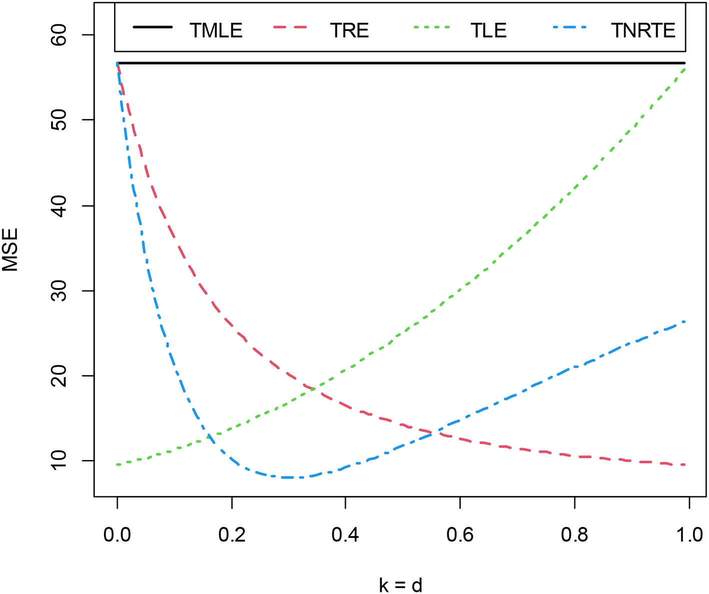
Figure 1. MSE of TMLE, TRE, TLE, and TNRTE for diffrent k, d.

Conclusions

In this study, we proposed the Tobit new ridge-type estimator (TNRTE) for overcoming the multicollinearity problem of the censored model. Theoretically, we compared the proposed TNRTE with some given estimators: the Tobit maximum likelihood estimator (TMLE), the Tobit ridge estimator (TRE), and the Tobit Liu estimator (TLE), and gave biasing parameter estimators of the proposed TNRTE. Then, a simulation study was performed to know the performance of the TMLE, the TRE, and the TLE with the proposed TNRTE. The results of the simulation indicate that the proposed TNRTE is better than other existing estimators in most cases. Moreover, real-life Mroz data were used to clarify the study results.

Data Availability Statement

The original contributions presented in the study are included in the article/supplementary material, further inquiries can be directed to the corresponding author.

Author Contributions

ID, MA, and FA contributed to conception and structural design of the manuscript. MA performed the simulation and application. All authors contributed to manuscript revision, read, and approved the submitted version.

Conflict of Interest

The authors declare that the research was conducted in the absence of any commercial or financial relationships that could be construed as a potential conflict of interest.

Publisher's Note

All claims expressed in this article are solely those of the authors and do not necessarily represent those of their affiliated organizations, or those of the publisher, the editors and the reviewers. Any product that may be evaluated in this article, or claim that may be made by its manufacturer, is not guaranteed or endorsed by the publisher.

Acknowledgments

The authors would like to thank the Deanship of Scientific Research at King Saud University represented by the Research Center at CBA for supporting this research financially.

References

1. Tobin J. Estimation of relationships for limited dependent variables. Econometrica. (1958) 26:24–36. doi: 10.2307/1907382

CrossRef Full Text | Google Scholar

2. Goldberger AS. Econometric Theory, 1st ed. New York, NY: John Wiley and Sons (1964), p. 1–399.

Google Scholar

3. Amemiya T. Tobit models: a survey. J Econom. (1984) 24:3–61. doi: 10.1016/0304-4076(84)90074-5

CrossRef Full Text | Google Scholar

4. Khalaf G, Mansson K, Sjolander P. A Tobit ridge regression estimator. Commun. Stat. Theory Methods. (2014) 43:131–40. doi: 10.1080/03610926.2012.655881

CrossRef Full Text | Google Scholar

5. Alhusseini FHH, Odah MH. Principal component regression for Tobit model and purchases of gold. In: Proceedings of the 10th International Management Conference, Bucharest, Romania. (2016) 10:491–500.

Google Scholar

6. Toker S, Özbay N, Siray GÜ, Yenilmez I. Tobit Liu estimation of censored regression model: an application to Mroz data and a Monte Carlo simulation study. J Stat Comput Simul. (2021) 91:1061–91. doi: 10.1080/00949655.2020.1828416

CrossRef Full Text | Google Scholar

7. Hoerl AE, Kennard RW. Ridge regression: biased estimation for nonorthogonal problems. Technometrics. (1970) 12:55–67. doi: 10.1080/00401706.1970.10488634

CrossRef Full Text | Google Scholar

8. Liu K. A new class of biased estimate in linear regression. Commun Stat Theory Methods. (1993) 22:393–402. doi: 10.1080/03610929308831027

CrossRef Full Text | Google Scholar

9. Kibria BMG, Lukman AF. A new ridge-type estimator for the linear regression model: simulations and applications. Hindawi. (2020) 2020:1–16. doi: 10.1155/2020/9758378

PubMed Abstract | CrossRef Full Text | Google Scholar

10. Lukman AF, Dawoud I, Kibria BM, Algamal ZY. A new ridge-type estimator for the gamma regression model. Scientifica. (2021) 2021:5545356. doi: 10.1155/2021/5545356

PubMed Abstract | CrossRef Full Text | Google Scholar

11. Lukman AF, Algamal ZY, Kibria BG. The KL estimator for the inverse Gaussian regression model. Concurr Comput Pract Exp. (2021) 33:e6222. doi: 10.1002/cpe.6222

CrossRef Full Text | Google Scholar

12. Akram MN, Kibria BG, Abonazel MR. On the performance of some biased estimators in the gamma regression model: simulation and applications. J Stat Comput Simul. (2022). doi: 10.1080/00949655.2022.2032059. [Epub ahead of print].

CrossRef Full Text | Google Scholar

13. Dawoud I, Abonazel MR. Generalized Kibria-Lukman estimator: method, simulation, and application. Front Appl Math Stat. (2022) 8:880086. doi: 10.3389/fams.2022.880086

PubMed Abstract | CrossRef Full Text

14. Awwad FA, Odeniyi KA, Dawoud I, Algamal ZY, Abonazel MRBM, Tag Eldin E. New two-parameter estimators for the logistic regression model with multicollinearity. WSEAS Trans Math. (2022) 21:403–14. doi: 10.37394/23206.2022.21.48

CrossRef Full Text | Google Scholar

15. Abonazel MR, Dawoud I, Awwad FA. Dawoud–Kibria estimator for beta regression model: simulation and application. Front Appl Math Stat. (2022) 8:775068. doi: 10.3389/fams.2022.775068

CrossRef Full Text | Google Scholar

16. Amemiya T. Regression analysis when the dependent variable is truncated normal. Econometrics. (1973) 41:997–1016. doi: 10.2307/1914031

CrossRef Full Text | Google Scholar

17. Fair RC. A note on computation of the Tobit estimator. Econometrics. (1977) 45:1723–7. doi: 10.2307/1913962

CrossRef Full Text | Google Scholar

18. Wang SG, Wu MX, Jia ZZ. Matrix Inequalities. 2^nd ed. Beijing: Chinese Science Press (2006), p. 1–116.

19. Farebrother RW. Further results on the mean square error of ridge regression. J R Stat Soc B. (1976) 38:248–50. doi: 10.1111/j.2517-6161.1976.tb01588.x

CrossRef Full Text | Google Scholar

20. Trenkler G, Toutenburg H. Mean squared error matrix comparisons between biased estimators-an overview of recent results. Stat Pap. (1990) 31:165–79. doi: 10.1007/BF02924687

CrossRef Full Text | Google Scholar

21. Kibria BMG. Performance of some new ridge regression estimators. Commun Stat Simul Comput. (2003) 32:419–35. doi: 10.1081/SAC-120017499

CrossRef Full Text | Google Scholar

22. Yenilmez I, Mert Kantar Y, Acitaş S. Estimation of censored regression model in the case of non-normal error. Sigma J Eng Nat Sci. (2018) 36:513–521.

Google Scholar

23. Yenilmez I, Mert Kantar Y. An alternative estimation method based on alpha skew logistic distribution for parameters of censored regression model. Data Sci Appl. (2019) 2:16–20.

Google Scholar

24. Yenilmez I, Ilhan U, Mert Kantar Y. Quasi-maximum likelihood estimator based on moyal distribution for censored data. In: 5th International Researchers, Statisticians and Young Statisticians Congress Aydin, Turkey. (2019), p. 419–27.

Google Scholar

25. Dawoud I, Abonazel MR. Robust Dawoud–Kibria estimator for handling multicollinearity and outliers in the linear regression model. J Stat Comput Simul. (2021) 91:3678–92. doi: 10.1080/00949655.2021.1945063

CrossRef Full Text | Google Scholar

26. Awwad FA Dawoud I, Abonazel MR. Development of robust Özkale–Kaçiranlar and Yang–Chang estimators for regression models in the presence of multicollinearity and outliers. Concurr Comput Pract Exp. (2022) 34:e6779. doi: 10.1002/cpe.6779

CrossRef Full Text | Google Scholar

27. Abonazel MR, Dawoud I. Developing robust ridge estimators for Poisson regression model. Concurr Comput Pract Exp. (2022) 34:e6979. doi: 10.1002/cpe.6979

CrossRef Full Text | Google Scholar

28. Algamal ZY, Abonazel MR. Developing a Liu-type estimator in beta regression model. Concurr Comput Pract Exp. (2022) 34:e6685. doi: 10.1002/cpe.6685

CrossRef Full Text | Google Scholar

29. Abonazel MR, Algamal ZY, Awwad FA, Taha IM. A New Two-parameter estimator for beta regression model: method, simulation, and application. Front Appl Math Stat. (2022) 7:780322. doi: 10.3389/fams.2021.780322

CrossRef Full Text | Google Scholar

30. Ozkale MR, Kaçiranlar S. The restricted and unrestricted two-parameter estimators. Commun Stat Theory Methods. (2007) 36:2707–25. doi: 10.1080/03610920701386877

CrossRef Full Text | Google Scholar

31. Mroz TA. The sensitivity of an empirical model of married women's hours of work to economic and statistical assumptions. Econometrica. (1987) 55:765–99. doi: 10.2307/1911029

CrossRef Full Text | Google Scholar

32. Barros M, Galea M, Leiva V. Generalized Tobit models: diagnostics and application in econometrics. J Appl Stat. (2018) 45:145–67. doi: 10.1080/02664763.2016.1268572

CrossRef Full Text | Google Scholar