Existence and uniqueness of solutions for stochastic urban-population growth model

1. Introduction

The Hokkaido prefecture, in Japan, had experienced a severe economic crisis that hit hard the social and living situation in that region [1]. Searching for better opportunities, individuals living in the countryside of that region started moving to the Sapporo city, capital of the Hokkaido prefecture. This migration led to an unbalance in Hokkaido's population distribution and created all kinds of social problems [1].

In an attempt to understand the population dynamics within the Hokkaido prefecture, a group of researchers has applied real-time population data to the so-called dynamic self-organization theory [see [1]]. This theory was first developed by Nicolis and Prigogine [2] in the classical monograph; this theory tries to explain a phenomenon in which a system organizes itself through internal and external interactions within the local population. The key idea is to let the interactions between two local populations be driven by a system of two deterministic differential equations. In formal terms, the deterministic differential equations are [e.g., [1]]

$\begin{array}{ll}\begin{array}{l}\frac{\text{ d}{x}_1(t)}{\text{d}t}=k_1{x}_1(t)(N_1-x_1(t)-\beta x_2(t))-d_1{x}_1(t),\hfill \\ \frac{\text{d}{x}_2(t)}{\text{d}t}=k_2{x}_2(t)(N_2-x_2(t)-\beta x_1(t))-d_2{x}_2(t),\hfill \end{array}& (1)\end{array}$

where x₁(t) and x₂(t) are positive terms that represent the population on the first and second region, respectively, and the constants k_i, N_i, and d_i, i = 1, 2, are positive and known constants. The constant β > 0 sets the interdependence level between the two regions [cf., [1]].

The authors of [1] have considered a linearization of the model (1) at the point $({\bar{x}}_1,{\bar{x}}_2)=(N_1-d_1/k_1,0)$, finding conditions for local stability, valid only around the point $({\bar{x}}_1,{\bar{x}}_2)$. Another study has shown that (1) has four different equilibrium points and that x_i(t), i = 1, 2, converges to one of these points as t increases to infinity [see [3]]. When reaching a convergence point, the two regions' population enters into equilibrium [cf., [3]]. In other words, the asymptotic stability of the system (1) is completely characterized by the authors of [3]. However, as pointed out in [[4], Chapter 5], the model in (1) remains incomplete because (1) does not account for random fluctuations that usually drive the behavior of population dynamics.

Researchers have become interested in stochastic differential equations for modeling population dynamics because these equations have proved to be useful in a variety of applications, such as in epidemics [5–7], fish population [8], phytoplankton concentration [9], HIV (virus) dynamics [10, 11], dengue [12], and tumor cell growth [13]. Researchers have even considered the stochastic version of the deterministic two-region population dynamics shown in (1) [e.g., [14–16]]. What researchers have proposed is, in fact, a stochastic model that simply adds the term σ_ix_i(t)dB_i(t), i = 1, 2, in (1), where B_i(t) denotes the standard unidimensional Brownian motion. The resulting stochastic differential equation is then studied in a way that the corresponding solution is unique [14–16]. To ensure uniqueness, the authors of [14–16] require that σ_i > 0, i = 1, 2; however, as we show in this paper, that condition is unnecessary—we show that σ_i, i = 1, 2, can be both positive and negative. This finding represents the main contribution of this paper.

The main contribution of this paper is to show the conditions that guarantee the stochastic urban-population growth model have a unique, positive solution. What this paper advances with respect to the previous results from the literature [e.g., [14–16]] is that this paper shows uniqueness and positiveness of solution without the classical assumption that σ_i > 0, i = 1, 2. This paper then expands the application of the result in [14–16] for the two-dimensional stochastic urban-population growth model. The main result of this paper is illustrated through a numerical simulation.

Notation: The set of (positive) real numbers is denoted by ℝ (ℝ₊), and the corresponding n-th dimensional (positive orthant) Euclidean space is denoted by ℝⁿ (${ℝ}_{+}^n$). Given two scalars x₁ and x₂, we define x₁∨x₂ = max(x₁, x₂) and x₁∧x₂ = min(x₁, x₂). The symbol |x| computes the Euclidean norm of x ∈ ℝⁿ. The symbol 𝟙_{·} stands for the Dirac measure. Every stochastic process studied in this paper evolves upon a fixed, filtered probability space $(\Omega ,{F},P)$.

2. Existence and uniqueness of the stochastic urban-population growth model

This section shows conditions to ensure the existence and uniqueness of solutions for the stochastic urban-population growth model. We emphasize that this paper is not the first to characterize the existence and uniqueness of solutions for such a system [e.g., [14–16]]; however, we show that a condition required by the authors of [14–16] is unnecessary, as detailed in the sequence.

The stochastic model studied in this paper arises from the Itô's extension of the system (1) with α_i = N_i−d_i/k_i, i = 1, 2, which equals

$\begin{array}{l}\text{d}{x}_i(t)=k_i\left({\alpha }_i{x}_i(t)-\beta x_1(t)x_2(t)-x_i^2(t)\right)\text{d}t+{\sigma }_i{x}_i(t)\text{d}{B}_i(t),\\ i=1,2,& (2)\end{array}$

where k_i, α_i, x_i(0), i = 1, 2, and β are positive, given scalars. In this paper, the constants σ_i ∈ ℝ, i = 1, 2, have no specific sign, in contrast to the studies in [14–16] that require σ_i > 0, i = 1, 2.

Now we recall the meaning of a solution for the system (2).

Definition 2.1 ([17], p. 48; [18], Definition 6.1.3, p. 101). We say x_i(t), i = 1, 2, is a solution for the system (2) if (i) {x_i(t)} is continuous and ${{F}}_t$-adapted, and (ii) the equation in (2) is valid for all t > 0 with probability one.

Remark 1. As proved in the monograph [[18], Coro. 6.3.2, p. 112] any stochastic differential equation with both drift term and diffusion term satisfying the locally Lipschitz condition has a solution within a bounded time frame [see also the proof of Theorem. 2.1 in [15] for a discussion]. As for the stochastic system (1), both the drift terms $x_i\mapsto k_i{\alpha }_i{x}_i-k_i\beta x_1{x}_2-k_i{x}_i^2$, i = 1, 2, and the diffusion terms x_i↦σ_ix_i, i = 1, 2, satisfy the local Lipschitz condition. Thus, the result in [[18], Coro. 6.3.2, p. 112] ensures that (2) has a solution x_i(t), i = 1, 2.

Definition 2.2. We say a solution x_i(t), i = 1, 2, is unique if any other solution ${\tilde{x}}_i(t)$, i = 1, 2, is indistinguishable from x_i(t), i = 1, 2, that is,

$\text{Pr}\left[x_i(t)={\tilde{x}}_i(t):i=1,2,\forall t>0\right]=1.$

Next, we introduce the concept of positive solution for the stochastic population model in (2).

Definition 2.3. We say the solution x_i(t), i = 1, 2, from (2) is positive if, given any initial condition x_i(0) ∈ ℝ₊, i = 1, 2, there holds

$\text{Pr}\left[x_i(t)\in {ℝ}_{+}:i=1,2,\forall t>0\right]=1.$

Now we can present the main result of this paper.

Theorem 2.1. The solution x_i(t), i = 1, 2, from (2) is both positive and unique.

The proof of Theorem 2.1 is postponed to Section 2.2.

Remark 2. The authors of [14–16] have attained the same result of Theorem 2.1 under the assumption that σ_i > 0, i = 1, 2; however, as stated in Theorem 2.1, this assumption is unnecessary. For this reason, Theorem 2.1 expands the usefulness of the result from [14–16] for the stochastic urban-population growth model as in (2).

2.1. Numerical simulation

This section illustrates the result of Theorem 2.1 through a simulation. In (1), we set x_i(0) = 0.5, σ_i = −1, i = 1, 2, k₁ = 0.2, k₂ = 0.3, α₁ = 0.6, α₂ = 0.5, and β = 0.5. We performed a Monte-Carlo simulation on (1) with one-thousand sample paths, each simulation taking 120 seconds. To simulate (1), we employed the Euler-Maruyama procedure as in [19] with step size of 10⁻⁵.

For all the Monte-Carlo samples taken randomly, we observed that both x₁(t) and x₂(t) were positive—this numerical evidence confirms the positiveness of the solution x_i(t), i = 1, 2, as discussed in Remark 1. Even though this positiveness is already characterized in the results of [14–16], these results apply only under the condition that σ_i > 0, i = 1, 2. This condition is unnecessary, as discussed in Remark 2; note that the numerical simulation suggested the result hold with σ_i = −1, i = 1, 2.

Figure 1 shows the corresponding mean and standard deviation taken for the minimum value between x₁(t) and x₂(t). The corresponding data indicate that both x₁(t) and x₂(t) are positive and unique, in accordance with Theorem 2.1.

FIGURE 1

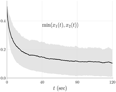
Figure 1. Mean (black) and standard deviation (light gray) curves of one thousand sample paths.

2.2. Proof of Theorem 2.1

Proof. The proof of Theorem 2.1 is divided into two parts. In the first part, we show that x_i(t), i = 1, 2, is positive; in the second part, we show that x_i(t), i = 1, 2, is unique.

Part I: the solution x_i(t), i = 1, 2, from (2) is positive for all t > 0.

To see that any solution x_i(t), i = 1, 2, satisfying (2) is positive, set i = 1 in (2) to write the identity

$\begin{array}{l}(\exp (-{\displaystyle {\int }_0^t(k_1{\alpha }_1-\beta k_1{x}_2(r)-k_1{x}_1(r))}\text{ d}r\\ -{\sigma }_1{\displaystyle {\int }_0^t\text{d}}{B}_1(r)))\frac{\text{d}{x}_1(t)}{\text{d}t}\\ =x_1(t)\left(k_1{\alpha }_1-k_1\beta x_2(t)-k_1{x}_1(t)+{\sigma }_1\frac{\text{d}{B}_1(t)}{\text{d}t}\right)\\ \times \exp \left(-{\displaystyle {\int }_0^t(k_1{\alpha }_1-\beta k_1{x}_2(r)-k_1{x}_1(r))}\text{ d}r-{\sigma }_1{\displaystyle {\int }_0^t\text{d}}{B}_1(r)\right).\end{array}$

Therefore,

$\begin{array}{l}\frac{\text{d}}{\text{d}t}(x_1(t)\exp (-{\displaystyle {\int }_0^t(k_1{\alpha }_1-\beta k_1{x}_2(r)-k_1{x}_1(r))}\text{d}r\\ -{\sigma }_1{\displaystyle {\int }_0^{\text{t}}\text{ d}}{B}_1(r)))=0,\end{array}$

which yields

$\begin{array}{l}{x}_1(t)=x_1(0)\exp ({\displaystyle {\int }_0^t(k_1{\alpha }_1-\beta k_1{x}_2(r)-k_1{x}_1(r))}\text{d}r\\ -{\sigma }_1{B}_1(t)).& (3)\end{array}$

It then follows from (3) that x₁(t) ∈ ℝ₊ for all t > 0 provided that x₁(0) ∈ ℝ₊. A similar reasoning applied in (2) with i = 2 shows that x₂(t) ∈ ℝ₊ for all t > 0 provided that x₂(0) ∈ ℝ₊. This argument proves that the stochastic system (2) has a positive solution provided that x_i(t) ∈ ℝ₊, i = 1, 2.

Part II: the solution x_i(t), i = 1, 2, from (2) is unique.

To prove the assertion of Part II, we begin with a change of variable upon (2). Namely, set u_i(t) = ln x_i(t), i = 1, 2, and apply upon them the Itô's formula [e.g., [17], p. 36, Theorem 6.4; [20], p. 48, Theorem 4.2.1] to obtain

$\begin{array}{l}\text{ d}{u}_i\left(t\right)=\text{d}ln{x}_i\left(t\right)\\ =\left(k_i{\alpha }_i-\frac{{\sigma }_i^2}{2}-\beta k_i{\displaystyle \sum _{j=1}^2}{1}_{i\ne j}{x}_j\left(t\right)-k_i{x}_i\left(t\right)\right)\text{ d}t\\ +{\sigma }_i\text{d}{B}_i\left(t\right),& (4)\end{array}$

with i = 1, 2. It follows that the solution u_i(t), i = 1, 2, from (4) is unique if and only if the solution x_i(t), i = 1, 2, from (2) is unique. From now on, we focus our analysis on the solution u_i(t), i = 1, 2, from (4).

Define $f_i:{ℝ}^2\mapsto ℝ$, i = 1, 2, as

$\begin{array}{lll}{f}_i(u_1,u_2)& =& k_i{\alpha }_i-\frac{{\sigma }_i^2}{2}-\beta k_i{\displaystyle \sum _{j=1}^2}{1}_{i\ne j}\exp (u_j)-k_i\exp (u_i),\\ \hfill i& =& 1,2.& (5)\end{array}$

As a result, the dynamics in (4) is identical to

$\begin{array}{ll}\text{d}{u}_i(t)=f_i(u_1(t),u_2(t))\text{d}t+{\sigma }_i\text{d}{B}_i(t),i=1,2,& (6)\end{array}$

with u_i(0) = ln x_i(0), i = 1, 2.

Now our task is to ensure that the solution u_i(t) has a finite growth whenever the time t > 0 is finite. To see that this finite growth holds, let us consider a constant η > 0 that satisfies |u|∨|v| ≤ η, where $u=(u_1,u_2)\in {ℝ}^2$ and $v=(v_1,v_2)\in {ℝ}^2$. As shown in the Appendix, there exists some constant c = c(η) > 0 such that

$\begin{array}{ll}{\displaystyle \underset{i=1,2}{max}}|f_i(u_1,u_2)-f_i(v_1,v_2){|}^2\le c(\eta )|u-v{|}^2,& (7)\end{array}$

that is, f_i, i = 1, 2, are locally Lipschitz continuous. Let u_i(t), v_i(t), i = 1, 2, be two solutions taken from (6). It follows from (6) that

$\begin{array}{ll}{u}_i(t)-v_i(t)={\displaystyle {\int }_{t_0}^t\left(f_i(u(s))-f(v(s)\right)}\text{ d}s,\forall t\ge t_0.& (8)\end{array}$

Applying the expected value operator on both sides of (8), together with the inequality in (7), we obtain (for all t ∈ [0, T] with given t > 0)

$\begin{array}{l}\text{E}\left[{\displaystyle \underset{t_0\le s\le t}{sup}}|u(s)-v(s){|}^2\right]\\ \le 2c(\eta )(T+4)\text{E}\left[{\displaystyle {\int }_0^t}{\displaystyle \underset{t_0\le r\le s}{sup}}|u(r)-v(r){|}^2\right]\text{ d}s.& (9)\end{array}$

Finally, the Grönwall's inequality applied in (9) yields [see [17], p. 53]

$\begin{array}{ll}\text{E}\left[{\displaystyle \underset{0\le t\le T}{sup}}|u(t)-v(t){|}^2\right]=0.& (10)\end{array}$

The identity in (10) means that u(t) = v(t) for all t ∈ [0, T], which means that the system (4) has a unique solution on the interval [0, T]. As a result, the solution x_i(t), i = 1, 2, from (2) is unique when t belongs to the interval [0, T].

It remains to show that x_i(t), i = 1, 2, is unique for all t > T when T increases toward infinity. To show this result, we consider the Lyapunov-like function $V:{ℝ}_{+}^2\mapsto {ℝ}_{+}$ as

$\begin{array}{ll}V(x)=x_1-ln(x_1)+x_2-ln(x_2),\forall x\in {ℝ}_{+}^2.& (11)\end{array}$

The idea is to use V(·) as in (11) to show that the solution x_i(t), i = 1, 2, from (2) cannot diverge to infinity while t is finite.

Using the Itô's formula [e.g., [17], p. 36, Theorem 6.4; [20], p. 48, Theorem 4.2.1] in both (2) and (11) yields

$\begin{array}{l}\text{d}V(x(t))={\displaystyle \sum _{i=1}^2}((x_i(t)-1)(k_i{\alpha }_i-k_i{x}_i(t)\\ -\beta k_i{\displaystyle \sum _{j=1}^2{1}_{i\cancel{=}j}}{x}_j(t))+\frac{{\sigma }_i^2}{2})\text{d}t\\ +{\sigma }_i(x_i(t)-1)\text{d}{B}_i(t).& (12)\end{array}$

Since both x₁(t) and x₂(t) are positive (see Part I), we can see that the right-hand side of (12) is bounded from above by

$\bar{\alpha }(x_1(t)+x_2(t)+1)\text{d}t+{\displaystyle \sum _{i=1}^2}{\sigma }_i(x_i(t)-1)\text{d}{B}_i(t),$

where

$\bar{\alpha }:=max\left\{1,{\displaystyle \sum _{i=1}^2}{k}_i\left({\alpha }_i+1+\beta +\frac{{\sigma }_i^2}{2}\right)\right\}.$

Taking the expected value operator on both sides of (12), we obtain

$\begin{array}{ll}\text{d}\text{E}\left[V(x(t))\right]\le \bar{\alpha }(\text{E}\left[x_1(t)+x_2(t)\right]+1)\text{d}t,\forall t\ge 0.& (13)\end{array}$

Since the expression x − 2 ln(x) is positive when x is positive (see Figure 2), we can write

$\begin{array}{ll}{\displaystyle \sum _{i=1}^2}\text{E}\left[x_i(t)\right]\le {\displaystyle \sum _{i=1}^2}\text{E}\left[2x_i(t)-2ln(x_i(t))\right].& (14)\end{array}$

Substituting (14) into the right-hand side of (13), and considering the definition of V(·) in (12), we can conclude that

$\begin{array}{ll}\text{d}\text{E}\left[V(x(t))\right]\le 2\bar{\alpha }(\text{E}\left[V(x(t))\right]+1/2)\text{d}t,\forall t\ge 0.& (15)\end{array}$

Finally, the solution of (15) satisfies

$\begin{array}{r}\text{E}\left[V(x(t))\right]\le \exp (2\bar{\alpha }t)V(x(0))+\frac{1}{2\bar{\alpha }}(\exp (2\bar{\alpha }t)-1),\\ \forall t\ge 0.& (16)\end{array}$

Even though the term 𝔼[V(x(t))] can increase when t increases, we now know from (16) that the growth of 𝔼[V(x(t))] is limited from above by an exponentially increasing curve. This curve ensures that (2) has a solution x_i(t), i = 1, 2, which cannot to diverge to infinity in finite time, as the next argument proves.

FIGURE 2

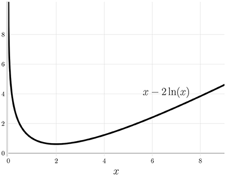
Figure 2. The curve indicates that x − 2 ln(x) is positive when x is positive.

To complete the proof, we proceed with a contradiction argument. Suppose from now on that there exists a finite number T_e>0 such that ${max}_{i=1,2}{x}_i(t)$ tends to infinity when t approaches T_e. Let t₀ > 0 be the time in which at least either x₁(t₀) or x₂(t₀) is greater than one. Define the stopping times

$\begin{array}{l}{T}_n=inf\left\{t\in [t_0,T_e):x_i(t)\notin (0,n]\text{ for some }i=1,2\right\},\\ \forall n>1.& (17)\end{array}$

It follows from (17) that

$\begin{array}{ll}{\displaystyle \underset{i=1,2}{max}}{x}_i(T_n)\to \infty \text{ as }n\to \infty ,& (18)\end{array}$

almost surely. Note that each stopping time T_n belongs to the interval [t₀, T_e) and T_e > 0 is assumed to be finite. In the next argument, we show that the sequence {T_n} diverges to infinity (almost surely) and, as a consequence, that T_e = ∞. Note that T_e = ∞ contradicts our initial assumption that T_e > 0 is finite.

Let us keep our initial assumption that T_e > 0 is finite. The fact that T_n < T_e for all n > 1 (almost surely) means that

$\begin{array}{ll}\text{Pr}\left[T_n<T_e\right]=1,\forall n>1.& (19)\end{array}$

Any realization (i.e., sample-path) of T_n, taken from the underlying sample space Ω, results from (17) that x(T_n)) > n − ln(n) for each n > 1. Thus,

$\begin{array}{ll}V(x(T_n))>n-ln(n),\forall n>1.& (20)\end{array}$

Combining (16), (19), and (20) yields

$\begin{array}{l}n-ln(n)<\text{E}\left[V(x(T_n))\right]\le \exp (2\bar{\alpha }{T}_e)V(x(0))\\ +\frac{1}{2\bar{\alpha }}\exp (2\bar{\alpha }{T}_e),\forall n>1,& (21)\end{array}$

which is absurd because the term on the left-hand side of (21) tends to infinity when n tends to infinity, while the term on the right-hand side of (21) remains finite. This contradiction proves that T_e = ∞, and as a result, the solution x_i(t), i = 1, 2, from (2) is unique for all t > 0.

3. Concluding remarks

This paper has shown conditions that ensure the positiveness and uniqueness of a stochastic urban-population growth model. This stochastic system has been studied in the literature for n-th dimensional systems [e.g., [14–16]], yet the results available so far require the diffusion constant σ_i be positive. As we have shown in Theorem 2.1, σ_i can be both positive and negative for two-dimensional systems (i.e., n = 2). For this reason, Theorem 2.1 can be seen as an extension of the results from [14–16] for two-dimensional systems.

The usefulness of Theorem 2.1 is illustrated through a Monte-Carlo simulation. The simulation was performed for the stochastic urban-population growth model with σ_i = −1, i = 1, 2 (see Section 2.1), and the corresponding data indicate that the system trajectories are both positive and unique—this numerical evidence confirms the novelty of Theorem 2.1.

Data availability statement

The original contributions presented in the study are included in the article/supplementary material, further inquiries can be directed to the corresponding author/s.

Author contributions

LB, HB, and MD made substantial contributions to the design of the work and generated the data. AV made the interpretation of data and revision of the text. All authors have read and approved the final manuscript.

Funding

Research supported in part by the Brazilian agencies CAPES grant 88881.030423/2013-01 and CNPq grant 305158/2017-1 and 401572/2016-1.

Conflict of interest

The authors declare that the research was conducted in the absence of any commercial or financial relationships that could be construed as a potential conflict of interest.

Publisher's note

All claims expressed in this article are solely those of the authors and do not necessarily represent those of their affiliated organizations, or those of the publisher, the editors and the reviewers. Any product that may be evaluated in this article, or claim that may be made by its manufacturer, is not guaranteed or endorsed by the publisher.

References

1. Miyata Y, Yamaguchi S. A study on Evolution of Regional Population Distribution Based on the Dynamic of Self-Organization Theory. Environmental Science, Hokkaido University (1990). p. 1–33.

Google Scholar

2. Nicolis G, Prigogine I. Self-Organization in Nonequilibrium Systems. Hoboken, NJ: John Wiley and Sons, Inc. (1977).

Google Scholar

3. El Ghordaf J, Hbid ML, Arino O. A mathematical study of a two-regional population growth model. Compt Rendus Biol. (2004) 327:977–82. doi: 10.1016/j.crvi.2004.09.006

PubMed Abstract | CrossRef Full Text | Google Scholar

4. May RM. Stability and Complexity in Model Ecosystems. Princeton, NJ: Princeton University Press (2019).

Google Scholar

5. Cai S, Cai Y, Mao X. A stochastic differential equation SIS epidemic model with two independent Brownian motions. J Math Anal Appl. (2019) 474:1536–50. doi: 10.1016/j.jmaa.2019.02.039

PubMed Abstract | CrossRef Full Text | Google Scholar

6. Zhao Y, Jiang D. The threshold of a stochastic SIS epidemic model with vaccination. Appl Math Comput. (2014) 243:718–27. doi: 10.1016/j.amc.2014.05.124

CrossRef Full Text | Google Scholar

7. Lu C, Liu H, Zhang D. Dynamics and simulations of a second order stochastically perturbed SEIQV epidemic model with saturated incidence rate. Chaos Solitons Fract. (2021) 152:111312. doi: 10.1016/j.chaos.2021.111312

CrossRef Full Text | Google Scholar

8. Yoshioka H, Yaegashi Y. Stochastic optimization model of aquacultured fish for sale and ecological education. J Math Indus. (2017) 7:1–23. doi: 10.1186/s13362-017-0038-8

CrossRef Full Text | Google Scholar

9. Møller JK, Madsen H, Carstensen J. Parameter estimation in a simple stochastic differential equation for phytoplankton modelling. Ecol Model. (2011) 222:1793–9. doi: 10.1016/j.ecolmodel.2011.03.025

CrossRef Full Text | Google Scholar

10. Dalal N, Greenhalgh D, Mao X. A stochastic model for internal HIV dynamics. J Math Anal Appl. (2008) 341:1084–101. doi: 10.1016/j.jmaa.2007.11.005

CrossRef Full Text | Google Scholar

11. Djordjevic J, Silva CJ, Torres DFM. A stochastic SICA epidemic model for HIV transmission. Appl Math Lett. (2018) 84:168–75. doi: 10.1016/j.aml.2018.05.005

CrossRef Full Text | Google Scholar

12. Din A, Khan T, Li Y, Tahir H, Khan A, Khan WA. Mathematical analysis of dengue stochastic epidemic model. Results Phys. (2021) 20:103719. doi: 10.1016/j.rinp.2020.103719

CrossRef Full Text | Google Scholar

13. Liu X, Li Q, Pan J. A deterministic and stochastic model for the system dynamics of tumor-immune responses to chemotherapy. Phys A Stat Mech Appl. (2018) 500:162–76. doi: 10.1016/j.physa.2018.02.118

CrossRef Full Text | Google Scholar

14. Du NH, Sam VH. Dynamics of a stochastic Lotka-Volterra model perturbed by white noise. J Math Anal Appl. (2006) 324:82–97. doi: 10.1016/j.jmaa.2005.11.064

CrossRef Full Text | Google Scholar

15. Mao X, Marion G, Renshaw E. Environmental Brownian noise suppresses explosions in population dynamics. Stochast Process Appl. (2002) 97:95–110. doi: 10.1016/S0304-4149(01)00126-0

CrossRef Full Text | Google Scholar

16. Mao X, Sabanis S, Renshaw E. Asymptotic behaviour of the stochastic Lotka-Volterra model. J Math Anal Appl. (2003) 287:141–56. doi: 10.1016/S0022-247X(03)00539-0

CrossRef Full Text | Google Scholar

17. Mao X. Stochastic Differential Equations and Applications. Cambridge: Woodhead Publishing (2008). doi: 10.1533/9780857099402

CrossRef Full Text | Google Scholar

18. Arnold L. Stochastic Differential Equations: Theory and Applications. Hoboken, NJ: Wiley-Interscience (1974).

Google Scholar

19. Higham DJ. An algorithmic introduction to numerical simulation of stochastic differential equations. SIAM Rev. (2001) 43:525–46. doi: 10.1137/S0036144500378302

CrossRef Full Text | Google Scholar

20. Oksendal B. Stochastic Differential Equations: An Introduction With Applications (Universitext). 5th Edn. Heidelberg; New York, NY: Springer-Verlag (2010).

Google Scholar

Appendix

The function $f_i:{ℝ}^2\mapsto ℝ$, i = 1, 2, defined in (5), reads as

$\begin{array}{lll}{f}_i(u_1,u_2)& =& k_i{\alpha }_i-\frac{k_i^2{\sigma }_i^2}{2}-\beta k_i{\displaystyle \sum _{j=1}^2}{1}_{i\ne j}\exp (u_j)-k_i^2\exp (u_i),\\ \hfill i& =& 1,2.\end{array}$

Hence,

$\begin{array}{l}{\displaystyle \underset{i=1,2}{max}}|f_i(u_1,u_2)-f_i(v_1,v_2){|}^2\le {\beta }^2{k}_1^2{(\exp (v_2)-\exp (u_2))}^2\\ +k_1^4{(\exp (v_1)-\exp (u_1))}^2+2\beta k_1^3(\exp (v_1)-\exp (u_1))\\ (\exp (v_2)-\exp (u_2))\\ +{\beta }^2{k}_2^2{(\exp (v_1)-\exp (u_1))}^2+k_2^4{(\exp (v_2)-\exp (u_2))}^2\\ +2\beta k_2^3(\exp (v_1)-\exp (u_1))(\exp (v_2)-\exp (u_2)).\end{array}$

After a simple algebraic manipulation, we can show that

$\begin{array}{r}{\displaystyle \underset{i=1,2}{max}}|f_i(u_1,u_2)-f_i(v_1,v_2){|}^2\\ \le [\beta (k_1^3+k_2^3)+({\beta }^2{k}_2^2+k_1^4)]{(\exp (v_1)-\exp (u_1))}^2\\ +[\beta (k_1^3+k_2^3)+({\beta }^2{k}_1^2+k_2^4)]{(\exp (v_2)-\exp (u_2))}^2.& (22)\end{array}$

Consider a constant η > 0 that satisfies |u|∨|v| ≤ η, where $u=(u_1,u_2)\in {ℝ}^2$ and $v=(v_1,v_2)\in {ℝ}^2$. According to the Lagrange finite-increments formula, there exists some constant ξ ∈ ℝ within the interval from ${min}_{i=1,2}(u_i\wedge v_i)$ to ${max}_{i=1,2}(u_i\vee v_i)$ such that |exp(v_i)−exp(u_i)| = exp(ξ)|v_i−u_i|. This fact, together with the inequality in (22), allows us to ensure the existence of some constant c = c(η) > 0 such that

$\begin{array}{ll}{\displaystyle \underset{i=1,2}{max}}|f_i(u_1,u_2)-f_i(v_1,v_2){|}^2\le c(\eta )|u-v{|}^2.& (23)\end{array}$

The inequality in (23) means that f_i, i = 1, 2, are locally Lipschitz continuous.