Restructured searls family of estimators of population mean in the presence of nonresponse

Introduction

Because of time and financial constraints, sampling is important when the population is big. Furthermore, many sampling studies use the mail questionnaire to acquire factual information due to financial constraints. The problem of nonresponse is common with mail questionnaires, and unexplained bias might be a major factor in these cases. Because of nonresponse, surveys may produce estimates that are biased with large variance. Nonresponse in a sample survey occurs when the inquirer is not able to get observations from some of the units of the population for a variety of reasons, including when someone refuses to answer, when respondents are unavailable, and the possibility that the respondents did not get the question due to a lack of interest or an inability to comprehend what was asked in the questionnaire. As a result, the researcher must be extra cautious when creating the survey questionnaire to ensure that such inaccuracies are minimized. Personal interviews often produce a more full response, although they are more expensive than the postal questionnaire approach. The goal of the investigator is to provide a system that incorporates the advantages of both strategies. When combining both strategies, the questionnaire form of the survey is typically addressed to larger targeted respondents rather than the size in need in the hope that the total returned forms will be larger than expected [1].

The most suitable estimator for any parameter under consideration is the related statistic when it comes to population parameter estimation. The sample mean of the primary variable, Y, for example, is the best estimator of the population mean, Ȳ. Although the estimator ȳ is unbiased for Ȳ, it has a significant sampling variance. As a result, we probed for a biased estimator with a lower mean squared error (MSE). This goal of finding a more efficient estimator is acquired by using an auxiliary variable that is highly associated with the main variable under study. When auxiliary variable,X is combined with data on Y to improve Ȳ estimation, it is expected that each sample unit has complete fact-based information on both variables and that they are accurately measured. However, it is a typical observation in many surveys that nonresponse happens in a variety of ways. Nonresponse can be caused by the refusal of the respondent to answer a specific question, their non-availability, information loss because of the negligence of the investigator or an accident, and lost observations. The most typical strategy for dealing with nonresponse to questionnaires is to have a personal interview with these nonrespondents in order to gather the maximum possible information. Many authors helped estimate Ȳ utilizing X with non-response for various nonresponse scenarios on Y and X.

Using mailed questionnaires, El-Badry [2] advocated estimating Ȳ of a research variate. Estimation of Ȳ through ratio, product, and regression estimators in the no response condition was examined by Rao and Khare and Srivastava [3–5]. Tracy and Osahan [6] explored how to get a better estimate of Ȳ with no response on Y and X. For the no response issue, [7] worked on a regression estimator for estimating Ȳ while [8] proposed an advanced estimation of Ȳ. Under the challenge of non-respond, [9] worked on a general class of exponential ratio estimators of Ȳ using transformed X. In a survey sample with replacement strategy, [10] proposed the estimation of Ȳ for random non-respond. In the context of nonrespond, [11] introduced an elevated ratio estimator for estimating Ȳ. For the issue of non-respond, [12] proposed an exponential type generalized estimator of Ȳ. While some observations on Y and X are missing, [13, 14] investigated the challenge of estimating the ratio of two Ȳ in survey sampling. In case of nonresponse, [15, 16] proposed employing multi-auxiliary characteristics to improve estimation of the ratio of the two Ȳ.

The estimation of Ȳ in a multi-phase sampling technique with nonresponse error was carried out by Srinath [17]. In a two-phase sampling design, [18, 19] proposed enhanced estimators of Ȳ with the problem of nonresponse. Shabbir and Khan [20] investigated estimating Ȳ, utilizing a known couple of X in double sampling in the presence of nonresponse. In a double sampling scheme, Yadav et al. [21] investigated the improved Ȳ estimation, utilizing the known parameters of Ȳ in the case of nonresponse and measurement errors. To overcome the challenge of measurement errors in sample surveys, Sud and Srivastava [22] and Srivastava and Shalabh [23] introduced the modified ratio and the regression type estimators of Ȳ. Kumar et al. [24] and Kumar [25] investigated the challenge of estimating Ȳ in the case of nonresponse and measurement error, and Singh et al. [26] worked on the same issue. In the case of nonrespose on Y along with X, [27] used the modified estimators with exponential functions for estimating Ȳ. Yadav et al. [28] worked on the problem of estimating Ȳ using information from highly correlated X in the face of nonresponse on one or both of the variables and proposed an improved estimator in three different nonresponse scenarios. Sharma and Kumar [29] proposed an estimator for estimating the Ȳ, with known parameters of X in sample surveys in the case of nonresponse. Unal and Kadilar [27] proposed the estimators class for estimating Ȳ, utilizing exponential function in the nonresponse condition for a couple of cases. In the condition of nonresponse on Y and X, Unal and Kadilar [27] adopted an exponential type estimator for Ȳ. Unal and Kadsilar [30] introduced a new class of exponential estimators in the case of nonresponse and Unal and Kadilar [31] worked on a novel population mean estimator for the nonresponse problem. Jaiswal et al. [32] suggested an elevated procedure for the estimation of population mean in the case of nonresponse. Some recent contributions for elevated estimation of Ȳ for the nonresponse problem were made by Ahmed at al. [33], Yadav et al. [34], Ahmed and Shabir [35], Hussain et al. [36], Unal and Kadilar [30], and Ahmad et al. [37].

The research studies showed that the estimators are getting better, as evidenced by decreasing MSE. The estimator with the sampling distribution having lower MSE was closer to the genuine, Ȳ. Thpresent investigation aimed to create an estimator that may enhance the true Ȳ estimation when there is a nonresponse error. We suggested a naive estimator of Ȳ, utilizing known information on X in the case of nonresponse error. We also noticed the large sample properties of the suggested estimator up to the first-degree approximation. The remainder of this study is laid out as below: The review of competing estimators is presented in Section Review of competing estimators, and introduced estimators are discussed in Section Proposed class of estimators. The suggested estimator is detailed in Section Efficiency conditions, while the efficiency comparison is discussed in Section Numerical illustrations. The numerical investigation is described in Section Simulation study, and the results and comments are presented in Sections Results and discussion and Conculsion, respectively.

Review of competing estimators

Hansen and Hurwitz [1] worked on the issue of nonresponse by introducing a novel subsampling procedure for the units which have not responded. In their technique, they considered that the population U = (U₁, U₂, ..., U_N) is the N finite and identifiable population units such that N = N₁ + N₂, where N₁ are the number of units with response and N₂ are the units with no response in the population respectively. Further a sample having n units is taken from the population under investigation using simple random sampling without replacement (SRSWOR) procedure. This sample is such that, n = n₁ + n₂, where n₁ have given response and n₂ has not given response in the sample. Let Y be the main characteristic under investigation and X as auxiliary variable. Further (y_i, x_i) are values on the i^th(i = 1, 2, ..., N) observations on Y and X for the population and a sub-sample of size $r=\frac{n_2}{h},(h>0)$ random observations from n₂ nonrespondents are taken with h as inverse sampling ratio for the sample from the second phase. The population's proportions of responders and nonresponders are, $W_1=\frac{N_1}{N}$ and $W_2=\frac{N_2}{N}$ respectively.

In the context of the nonresponse issue, Hansen and Hurwitz [1] suggested the unbiased estimator of Ȳ as,

$\begin{array}{l}{t}_1=w_1{ȳ}_1+w_2{ȳ}_{2(r)}\end{array}$

Where, $w_1=\frac{n_1}{n}$ and $w_2=\frac{n_2}{n}$ are the sample proportions of responders and nonresponders respectively with the ȳ₁ and ȳ_2(r) as the sample means for n₁ and r units for the respondents and nonrespondents respectively.

The sampling variance of t₁ for the approximation of first order is,

$\begin{array}{ll}V(t_1)={Ȳ}^2\left[\lambda C_y^2+\frac{W_2(h-1)}{n}{C}_{y(2)}^2\right]& (1)\end{array}$

where

$\lambda =\frac{1-f}{n}$, $f=\frac{n}{N}$, $C_y^2=\frac{S_y^2}{{Ȳ}^2}$ and $C_{y(2)}^2=\frac{S_{y(2)}^2}{{Ȳ}^2}$ is the square of the coefficient of variation (CV) of Y for the N₂ population's nonresponders.

It is very common phenomenon in practice that we face the issue of nonrespond on Yand X both. In the present investigation, we are dealing with the issue of nonrespond on Y and X both.

Singh et al. [38] introduced the traditional ratio estimator of Ȳ with the non-respond on Y and X, utilizing the known $\stackrel{-}{X}$ and having high positive correlation between Y and X as,

$\begin{array}{l}{t}_2=\frac{{ȳ}^{*}}{{\stackrel{-}{x}}^{*}}\stackrel{-}{X}\end{array}$

Where, ${ȳ}^{*}=\frac{1}{n-r}{\displaystyle \sum _{i=1}^{n-r}}{y}_i$ and ${\stackrel{-}{x}}^{*}=\frac{1}{n-r}{\displaystyle \sum _{i=1}^{n-r}}{x}_i$

The MSE of t₂ till the approximation of degree one is,

$\begin{array}{l}MSE(t_2)={Ȳ}^2[\lambda (C_y^2+C_x^2-2C_{yx})+\frac{W_2(h-1)}{n}(C_{y(2)}^2\\ +C_{x(2)}^2-2C_{yx(2)})]& (2)\end{array}$

where

$C_x^2=\frac{S_x^2}{{\stackrel{-}{X}}^2}$, C_yx = ρ_yxC_yC_x, $C_{x(2)}^2=\frac{S_{x(2)}^2}{{\stackrel{-}{X}}^2}$, C_yx(2) = ρ_yx(2)C_y(2)C_x(2) with the ρ_yx and ρ_yx(2) as the population correlation coefficients for the respondents and nonrespondents, respectively.

Searls [39] worked on the exponential ratio estimator with the nonresponse on Y and X both and having somewhat weak positive correlation between Y and X as,

$\begin{array}{l}{t}_3={ȳ}^{*}exp\left(\frac{\stackrel{-}{X}-{\stackrel{-}{x}}^{*}}{\stackrel{-}{X}+{\stackrel{-}{x}}^{*}}\right)\end{array}$

The MSE of t₃ for the approximation of order one is,

$\begin{array}{l}MSE(t_3)={Ȳ}^2[\lambda (C_y^2+\frac{C_x^2}{4}-C_{yx})+\frac{W_2(h-1)}{n}(C_{y(2)}^2\\ +\frac{C_{x(2)}^2}{4}-C_{yx(2)})]& (3)\end{array}$

Singh et al. [38] worked on the usual regression estimator for the problem of nonrespond on Y and X presented estimator as,

$\begin{array}{l}{t}_4={ȳ}^{*}+b^{*}(\stackrel{-}{X}-{\stackrel{-}{x}}^{*})\end{array}$

Where, $b^{*}=\frac{s_{yx}^{*}}{s_x^{*2}}$ is the sample regression coefficient of the regression line of Y and X for the nonrespondents in the sample.

The MSE of t₄ for the approximation of degree one is,

$\begin{array}{l}MSE(t_4)={Ȳ}^2[\lambda C_y^2(1-{\rho }_{yx}^2)+\frac{W_2(h-1)}{n}\{C_{y(2)}^2\\ +{\rho }_{yx}^2\frac{C_y^2}{C_x^2}{C}_{x(2)}^2-2{\rho }_{yx}\frac{C_y}{C_x}{C}_{yx(2)}\}]& (4)\end{array}$

where, C_yx(2) = ρ_yx(2)C_y(2)C_x(2)

Unal and Kadilar [27] worked on the following modified exponential ratio estimator of Ȳ with the issue of nonrespond on both Y and X as,

$\begin{array}{l}{t}_5=\alpha {ȳ}^{*}+(1-\alpha ){ȳ}^{*}exp\left(\frac{\stackrel{-}{X}-{\stackrel{-}{x}}^{*}}{\stackrel{-}{X}+{\stackrel{-}{x}}^{*}}\right)\end{array}$

The MSE of t₅ for the approximation of order one is,

$\begin{array}{l}MSE(t_5)=\\ {Ȳ}^2\left[\begin{array}{l}\left\{\lambda C_y^2+\frac{W_2(h-1)}{n}\{C_{y(2)}^2\right\}+\left\{\lambda C_x^2+\frac{W_2(h-1)}{n}{C}_{x(2)}^2\right\}\left(\frac{{\alpha }^2}{4}-\frac{\alpha }{2}+\frac{1}{4}\right)\\ +\left\{\lambda {\rho }_{yx}{C}_y{C}_x+\frac{W_2(h-1)}{n}{\rho }_{yx(2)}{C}_{y(2)}{C}_{x(2)}\right\}(1-\alpha )\end{array}\right]& (5)\end{array}$

The optimal α for which the MSE of t₅ is least is,

$\begin{array}{l}\alpha =\frac{A_1-2A_2}{A_1}={\alpha }_{opt}\end{array}$

Where, $A_1=\lambda C_x^2+\frac{W_2(h-1)}{n}\{C_{y(2)}^2$ and $A_2=\lambda C_{yx}+\frac{W_2(h-1)}{n}{\rho }_{yx(2)}{C}_{y(2)}{C}_{x(2)}$

The least MSE of t₅ for the optimal α is,

$\begin{array}{l}MS{E}_{min}(t_5)={Ȳ}^2[\left\{\lambda C_y^2+\frac{W_2(h-1)}{n}\{C_{y(2)}^2\right\}\\ -\frac{{\left\{\lambda C_{yx}+\frac{W_2(h-1)}{n}{\rho }_{yx(2)}{C}_{y(2)}{C}_{x(2)}\right\}}^2}{\left\{\lambda C_x^2+\frac{W_2(h-1)}{n}{C}_{x(2)}^2\right\}}]& (6)\end{array}$

Proposed class of estimators

Motivated by Khare and Kumar [40] and Unal and Kadilar [27], we introduced the following modified generalized class for enhanced estimation of Ȳ with the problem of nonresponse on Y and X as

$\begin{array}{l}{t}_p={\pi }_1{ȳ}^{*}+{\pi }_2{ȳ}^{*}exp\left(\frac{\stackrel{-}{X}-{\stackrel{-}{x}}^{*}}{\stackrel{-}{X}+{\stackrel{-}{x}}^{*}}\right),\end{array}$

where, π₁ and π₂ (π₁ + π₂ ≠ 1) are the characterizing scalars that are obtained such that the MSE of t_p is least possible.

Following are some of the interesting observations about the introduced family of estimators:

(1) For π₁ = 1 and π₂ = 0, the proposed class becomes ȳ^* estimator of Ȳ with the issue of nonresponse.

(2) For π₂ = 0, the suggested family of estimators reduces to the estimator introduced by Khare and Kumar [40] with the problem of nonresponse.

(3) For π₁ = 0 and π₂ = 1, the introduced class of estimators takes the form of the exponential ratio estimator of ȳ introduced by Searls [39] for the problem of nonresponse.

(4) For π₁ + π₂ = 1, the suggested family reduces to the class of estimators of Ȳ introduced by Unal and Kadilar [27] for the issue of nonresponse.

For sampling properties of the introduced estimator, t_p, we used the standard notations given below:

${ȳ}^{*}=Ȳ(1+e_0^{*})$ and ${\stackrel{-}{x}}^{*}=\stackrel{-}{X}(1+e_1^{*})$ with $E(e_0^{*})=E(e_1^{*})=0$ and $E(e_0^{*2})=\lambda C_y^2+\frac{W_2(h-1)}{n}{C}_{y(2)}^2$, $E(e_1^{*2})=\lambda C_x^2+\frac{W_2(h-1)}{n}{C}_{x(2)}^2$, $E(e_0^{*}{e}_1^{*})=\lambda C_{yx}+\frac{W_2(h-1)}{n}{C}_{yx(2)}$

Expressing t_p in terms of $e_i^{*}$(i = 0, 1), we have

$\begin{array}{r}{t}_p={\pi }_1Ȳ(1+e_0^{*})+{\pi }_2Ȳ(1+e_0^{*})(1-\frac{e_1^{*}}{2}+\frac{3}{8}{e}_1^{*2})\\ ={\pi }_1Ȳ(1+e_0^{*})+{\pi }_2Ȳ(1+e_0^{*}-\frac{e_1^{*}}{2}-\frac{e_0^{*}{e}_1^{*}}{2}+\frac{3}{8}{e}_1^{*2})\\ =Ȳ\left[{\pi }_1(1+e_0^{*})+{\pi }_2(1+e_0^{*}-\frac{e_1^{*}}{2}-\frac{e_0^{*}{e}_1^{*}}{2}+\frac{3}{8}{e}_1^{*2})\right]\end{array}$

Subtracting Ȳ from two sides of above equation, we have,

$\begin{array}{l}{t}_p-Ȳ\\ =Ȳ\left[{\pi }_1(1+e_0^{*})+{\pi }_2(1+e_0^{*}-\frac{e_1^{*}}{2}-\frac{e_0^{*}{e}_1^{*}}{2}+\frac{3}{8}{e}_1^{*2})-1\right]& (7)\end{array}$

By taking expectations on two sides of (7) and substituting the values of corresponding expectations, we have the bias of t_p as

$\begin{array}{l}Bias(t_p)=Ȳ[{\pi }_1+{\pi }_2(1-\frac{1}{2}\left\{\lambda C_{yx}+\frac{W_2(h-1)}{n}{C}_{yx(2)}\right\}\\ +\frac{3}{8}\left\{\lambda C_y^2+\frac{W_2(h-1)}{n}{C}_{y(2)}^2\right\})-1]\end{array}$

Squaring on both sides of (7), simplifying and occluding the terms for the approximation of degree one, we get

$\begin{array}{l}{(t_p-Ȳ)}^2\\ ={Ȳ}^2\left[\begin{array}{l}1+{\pi }_1^2(1+e_0^{*2})+{\pi }_2^2(1+e_0^{*2}+e_1^{*2}-2e_0^{*}{e}_1^{*})-2{\pi }_1\\ -2{\pi }_2(1+\frac{3}{8}{e}_1^{*2}-\frac{e_0^{*}{e}_1^{*}}{2})+2{\pi }_1{\pi }_2(1+e_0^{*2}+\frac{3}{8}{e}_1^{*2}-e_0^{*}{e}_1^{*})\end{array}\right]\end{array}$

By taking expectations on two sides of the above equation and substituting the values of corresponding expectations, we obtain the MSE of t_p as

$\begin{array}{l}MSE(t_p)=\\ {Ȳ}^2\left[\begin{array}{l}1+{\pi }_1^2\left(1+\left\{\lambda C_y^2+\frac{W_2(h-1)}{n}{C}_{y(2)}^2\right\}\right)\\ +{\pi }_2^2(1+\left\{\lambda C_y^2+\frac{W_2(h-1)}{n}{C}_{y(2)}^2\right\}\\ +\left\{\lambda C_x^2+\frac{W_2(h-1)}{n}{C}_{x(2)}^2\right\}-2\left\{\lambda C_{yx}+\frac{W_2(h-1)}{n}{C}_{yx(2)}\right\})\\ -2{\pi }_1-2{\pi }_2(1+\frac{3}{8}\left\{\lambda C_x^2+\frac{W_2(h-1)}{n}{C}_{x(2)}^2\right\}\\ -\frac{1}{2}\left\{\lambda C_{yx}+\frac{W_2(h-1)}{n}{C}_{yx(2)}\right\})\\ +2{\pi }_1{\pi }_2(1+\left\{\lambda C_y^2+\frac{W_2(h-1)}{n}{C}_{y(2)}^2\right\}\\ +\frac{3}{8}\left\{\lambda C_x^2+\frac{W_2(h-1)}{n}{C}_{x(2)}^2\right\}-\left\{\lambda C_{yx}+\frac{W_2(h-1)}{n}{C}_{yx(2)}\right\})\end{array}\right]\\ MSE(t_p)={Ȳ}^2\left[1+{\pi }_1^{2}A+{\pi }_2^{2}B-2{\pi }_1-2{\pi }_{2}C+2{\pi }_1{\pi }_{2}D\right]& (8)\end{array}$

where

$\begin{array}{l}A=\left(1+\left\{\lambda C_y^2+\frac{W_2(h-1)}{n}{C}_{y(2)}^2\right\}\right),\\ B=(1+\left\{\lambda C_y^2+\frac{W_2(h-1)}{n}{C}_{y(2)}^2\right\}\\ +\left\{\lambda C_x^2+\frac{W_2(h-1)}{n}{C}_{x(2)}^2\right\}\\ -2\left\{\lambda C_{yx}+\frac{W_2(h-1)}{n}{C}_{yx(2)}\right\}),\\ C=(1+\frac{3}{8}\left\{\lambda C_x^2+\frac{W_2(h-1)}{n}{C}_{x(2)}^2\right\}\\ -\frac{1}{2}\left\{\lambda C_{yx}+\frac{W_2(h-1)}{n}{C}_{yx(2)}\right\}),\\ D=(1+\left\{\lambda C_y^2+\frac{W_2(h-1)}{n}{C}_{y(2)}^2\right\}\\ +\frac{3}{8}\left\{\lambda C_x^2+\frac{W_2(h-1)}{n}{C}_{x(2)}^2\right\}\\ -\left\{\lambda C_{yx}+\frac{W_2(h-1)}{n}{C}_{yx(2)}\right\})\end{array}$

The optimal π₁ and π₂ values which minimizes the MSE of t_p respectively are,

$\begin{array}{l}{\pi }_{1(opt)}=\frac{(B-DC)}{(AB-D^2)}\text{ and }{\pi }_{2(opt)}=\frac{(AC-D)}{(AB-D^2)}\end{array}$

The least MSE of t_p for these optimal π₁ and π₂ is,

$\begin{array}{l}MS{E}_{min}(t_p)=\\ {Ȳ}^2\left[1-\frac{\left\{\begin{array}{l}2(B-DC)(AB-D^2)+2(AC-D)(AB-D^2)\\ -B{(AC-D)}^2-A{(B-DC)}^2+2D(B-DC)(AC-D)\end{array}\right\}}{{(AB-D^2)}^2}\right]\end{array}$

$\begin{array}{ll}MS{E}_{min}(t_p)={Ȳ}^2\left[1-\frac{P}{Q^2}\right]& (9)\end{array}$

Where,

$\begin{array}{l}P=\left\{\begin{array}{l}2(B-DC)(AB-D^2)+2(AC-D)(AB-D^2)\\ -B{(AC-D)}^2-A{(B-DC)}^2+2D(B-DC)(AC-D)\end{array}\right\}\\ Q=(AB-D^2)\end{array}$

Efficiency conditions

The efficiency of the proposed and competing estimators have been compared theoretically in the case of nonresponse on both Y and X showed that the efficiency condition of the suggested estimator is superior to the competing estimators. The MSEs of the estimators are used to assess their efficiency. Any estimator t_a is said to be more efficient or better than the estimator, t_b, if the condition MSE(t_b) − MSE(t_a) > 0 is satisfied.

The suggested estimator t₁ performs better than the estimator proposed by Hansen and Hurwitz [1] under the condition:

if V(t₁) − MSE(t_p) > 0, or

$\begin{array}{l}\left[\lambda C_y^2+\frac{W_2(h-1)}{n}{C}_{y(2)}^2\right]-\left[1-\frac{P}{Q^2}\right]>0,or\end{array}$

$\begin{array}{l}\left[\lambda C_y^2+\frac{W_2(h-1)}{n}{C}_{y(2)}^2+\frac{P}{Q^2}\right]>1\end{array}$

The proposed estimator t_p has lesser MSE than the estimator t₂ proposed by Ahmed and Shabeer [35] for the following condition:

if MSE(t₂) − MSE_min(t_p) > 0, or

$\begin{array}{l}\left[\lambda (C_y^2+C_x^2-2C_{yx})+\frac{W_2(h-1)}{n}(C_{y(2)}^2+C_{x(2)}^2-2C_{yx(2)})\right]\\ -\left[1-\frac{P}{Q^2}\right]>0,or\end{array}$

$\begin{array}{l}[\lambda (C_y^2+C_x^2-2C_{yx})+\frac{W_2(h-1)}{n}(C_{y(2)}^2+C_{x(2)}^2-2C_{yx(2)})\\ \\ +\frac{P}{Q^2}]>0\end{array}$

The introduced estimator t_p is more efficient than the exponential ratio estimator t₃ proposed by Yadav et al. [34] under the following condition:

if MSE(t₃) − MSE_min(t_p) > 0, or

$\begin{array}{l}\left[\lambda (C_y^2+\frac{C_x^2}{4}-C_{yx})+\frac{W_2(h-1)}{n}(C_{y(2)}^2+\frac{C_{x(2)}^2}{4}-C_{yx(2)})\right]\\ -\left[1-\frac{P}{Q^2}\right]>0,\text{or}\end{array}$

$\begin{array}{l}[\lambda (C_y^2+\frac{C_x^2}{4}-C_{yx})+\frac{W_2(h-1)}{n}(C_{y(2)}^2+\frac{C_{x(2)}^2}{4}-C_{yx(2)})\\ +\frac{P}{Q^2}]>1\end{array}$

The introduced estimator t_p outperforms the competitor's estimator t₄ of Ahmed and Shabeer [35] under the following condition:

if MSE(t₄) − MSE_min(t_p) > 0, or

$\begin{array}{l}[\lambda C_y^2(1-{\rho }_{yx}^2)+\frac{W_2(h-1)}{n}\{C_{y(2)}^2+{\rho }_{yx}^2\frac{C_y^2}{C_x^2}{C}_{x(2)}^2\\ -2{\rho }_{yx}\frac{C_y}{C_x}{C}_{yx(2)}\}]-\left[1-\frac{P}{Q^2}\right]>0,\text{or}\end{array}$

$\begin{array}{l}[\lambda C_y^2(1-{\rho }_{yx}^2)+\frac{W_2(h-1)}{n}\{C_{y(2)}^2+{\rho }_{yx}^2\frac{C_y^2}{C_x^2}{C}_{x(2)}^2\\ -2{\rho }_{yx}\frac{C_y}{C_x}{C}_{yx(2)}\}+\frac{P}{Q^2}]>1\end{array}$

The proposed estimator t_p has lesser MSE than the estimator t₅ proposed by Unal and Kadilar [27] for the following stipulation:

if MSE(t₅) − MSE_min(t_p) > 0, or

$\begin{array}{l}[\left\{\lambda C_y^2+\frac{W_2(h-1)}{n}\{C_{y(2)}^2\right\}\\ -\frac{{\left\{\lambda C_{yx}+\frac{W_2(h-1)}{n}{\rho }_{yx(2)}{C}_{y(2)}{C}_{x(2)}\right\}}^2}{\left\{\lambda C_x^2+\frac{W_2(h-1)}{n}{C}_{x(2)}^2\right\}}]\\ -\left[1-\frac{P}{Q^2}\right]>0,\text{or}\end{array}$

$\begin{array}{l}[\left\{\lambda C_y^2+\frac{W_2(h-1)}{n}\{C_{y(2)}^2\right\}\\ -\frac{{\left\{\lambda C_{yx}+\frac{W_2(h-1)}{n}{\rho }_{yx(2)}{C}_{y(2)}{C}_{x(2)}\right\}}^2}{\left\{\lambda C_x^2+\frac{W_2(h-1)}{n}{C}_{x(2)}^2\right\}}+\frac{P}{Q^2}]>1\end{array}$

Numerical illustrations

In this section, the theoretical efficiency conditions were verified using five real natural data congregations. To see the executions of the introduced and the competing estimators of Ȳ in the presence of nonresponse on both Yand X, we considered all five natural real populations [27]. The parameters of all five considered populations along with their sources are presented in Table 1.

TABLE 1

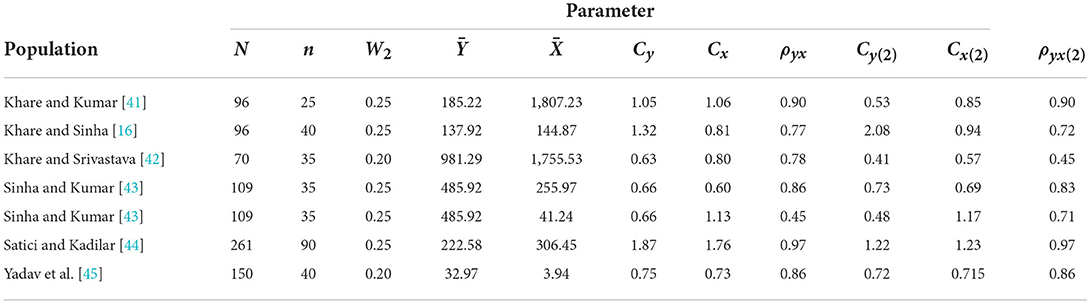
Table 1. Parameters of different populations under consideration.

All the above seven populations under consideration were natural real-world populations on which the applications of the suggested estimator along with the competing estimators were carried out in the presence of nonresponse. For instance, we described the seven real-world populations in Yadav et al.'s study [45] as follows:

The data were collected from 923 districts of Turkey from different private teaching institutions in 2006. The study variable Ywas taken as the number of successful students in the student selection examination for secondary schools and the auxiliary variableXwas taken as the number of teachers. It should be mentioned that only 261 homogenous districts for the above population were considered as we used simple random sampling in this study and a sample of size 90 was drawn from the above population of size 261. Here, we faced the problem of nonresponse in both the study and the auxiliary variables. A total of 25% of the units (65 units) was represented in the group of nonresponse.

In the last population, the primary data set, also presented in Yadav et al. [45], for simple random sampling on the production of peppermint yield, which is located at Banikodar block of Barabanki district at Uttar Pradesh state in India in 2019, was collected. It was observed that approximately 20% of nonresponse occurred while collecting data for the targeted units of the population under consideration, and the data were collected on 150 farmers with peppermint yield as the primary variable in kilogram and the auxiliary variable as an area of the field in Bigha (2529.3 Square Meter). Thus, out of 150 units, 120 units were considered in the response group and 20 in the nonresponse group. The parameters of this population are presented in Table 1.

The percentage relative efficiency (PRE) of the suggested and competing estimators with respect to the estimator t₁ was calculated using the following formula:

$\begin{array}{l}PRE(t_i)=\frac{MSE(t_1)}{MSE(t_i)}\times 100,i=1,2,...,5,p\end{array}$

The percentage relative efficiencies of the suggested estimator t_p and competing estimators over t₁ for all five populations for different values of hare presented in Tables 2–8.

TABLE 2

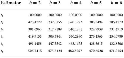
Table 2. Percentage relative efficiency (PRE) of different estimators with respect to t₁ for Population 1.

Simulation study

To visualize the performances of the introduced and the competing estimators on the large population, we generated a large artificial population. A simulated population was generated through the R programming language to compare the outcomes of competing estimators and the introduced estimator for the artificial population. For the simulated population, we used the parameters of the real Population 1 given in the numerical study section. A bivariate normal distribution with mean vectors and a variance-covariance matrix to construct the population are as follows:

Means of [Y, X] as μ = [185.22, 1807.23]

$\begin{array}{l}\text{Variances and covariance of }\left[\text{Y},\text{ X}\right]\text{ as }{\text{σ}}^2=\\ \left[\begin{array}{cc}37822.86& 335303.53\\ 335303.53& 3669767.79\end{array}\right]\end{array}$

Correlation ρ_yx = 0.90

The following steps were used for the simulation of the required population:

(a) A bivariate normal distribution of X and Y of size N = 5000 has been generated through these parameters using the R Program.

(b) The parameters have been computed for this simulated population of size N = 5000 with N₁ = 3500 and N₂ = 1500.

(c) A sample of size n with n₁ and n₂ = n − n₁ has been selected from this simulated population.

(d) Sample statistics, which are the sample mean, sample variance, and the values of the introduced and competing estimators t_i of Ȳ, are calculated for this sample.

(e) Steps (c) and (d) are repeated m = 50, 000 times.

(f) The MSE of every estimator t_i is calculated using the formula, $MSE(t_i)=\frac{1}{m}{\displaystyle \sum _{j=1}^m}{(t_{ij}-Ȳ)}^2$.

(g) The PRE of each of the estimator t_i with respect to t₁ has been calculated using the formula:

$\begin{array}{l}PRE(t_i)=\frac{MSE(t_1)}{MSE(t_i)}\times 100,i=1,2,...,5,p\end{array}$

Table 9 represents the PRE of different estimators of Ȳ with respect to t₁ for the simulated population.

Results and discussion

It can be verified from Table 2 that the PREs of the competing estimators over t₁ lie in the intervals [301.6963, 491.1458], [310.1851, 463.1675], [306.3844, 447.5542], [276.1563, 438.3615], and [254.0789, 432.8506] for different values of h from 2 to 6, respectively, for Population 1. From Table 3, it can be observed that the PREs of the estimators in competition over the estimator t₁ lie in the intervals [148.0884, 220.6768], [144.4216, 214.9752], [142.6821, 212.6081], [141.6667, 211.3493], and [141.0011, 210.5799] for different values of h from 2 to 6, respectively, for Population 2. It can be verified from Table 4 that the PREs of the competing estimators over t₁ lie in the intervals [124.3555, 210.8401], [108.5754, 189.2205], [98.8639, 176.1734], [92.2849, 167.4633], and [87.5332, 161.2454] for different values of h from 2 to 6, respectively, for Population 3. It can be observed from Table 5 that the PREs of the competing estimators over t₁ lie in the intervals [233.9950, 359.4776], [232.7577, 351.3462], [232.0054, 346.5934], [231.4997, 343.4756], and [231.1363, 341.2729] for different values of h from 2 to 6, respectively, for Population 4. It can be verified from Table 6 that the PREs of the competing estimators over t₁ estimator lie in the intervals [38.8760, 133.8633], [37.0780, 140.6118], [35.8300, 146.1823], [34.9130, 150.8558], and [34.2109, 154.8319] for different values of h from 2 to 6, respectively, for Population 5. From Table 7, it is evident that the PREs of the competing estimators over t₁ estimator lie in the intervals [334.7728, 1735.3152], [340.5247, 1739.5428], [346.0438, 1745.3751], [351.8249, 1749.6817], and [357.4681, 1754.8894] for different values of h from 2 to 6, respectively, for Population 6. From Table 8, it can be observed that the PREs of the competing estimators over the estimator t₁ lie in the intervals [150.5897, 383.9387], [125.4893, 383.8675], [118.8892, 383.8323], [115.8396, 383.8108], and [114.0844, 383.7792] for different values of h from 2 to 6, respectively, for Population 7. The PREs of the competing estimators with respect to t₁ for the simulated population for different values of h from 2 to 6 lie in the interval [269.1084, 502.3164]. On the other hand, the PREs of the introduced estimator over t₁ for different values of h from 2 to 6, respectively, are (506.2415, 482.3257, 473.5124, 470.6528, and 471.0254) for Population 1, (228.4691, 225.3594, 224.2563, 222.2874, and 221.9566) for Population 2, (223.4526, 215.2046, 188.8459, 183.9876, and 181.0087) for Population 3, (418.5783, 416.6584, 414.6217, 412.5894, and 412.01365) for Population 4, (139.2657, 151.4568, 157.3259, 163.4628, and 168.8413) for Population 5, (2054.8142, 2066.5743, 2074.2057, 2083.9104, 2087.7764) for Population 6, and (454.8142, 454.5743, 453.8057, 453.6104, and 452.7764) for Population 7. The PREs of the competing estimators with respect to t₁ for the simulated population for different values of from 2 to 6 lie in the interval [483.2057, 529.9382].

TABLE 3

Table 3. PRE of different estimators with respect to t₁ for Population 2.

TABLE 4

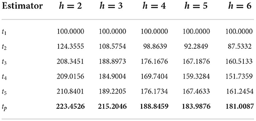
Table 4. PRE of different estimators with respect to t₁ for Population 3.

TABLE 5

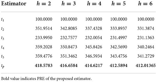
Table 5. PRE of different estimators with respect to t₁ for Population 4.

TABLE 6

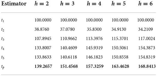
Table 6. PRE of different estimators with respect to t₁ for Population 5.

TABLE 7

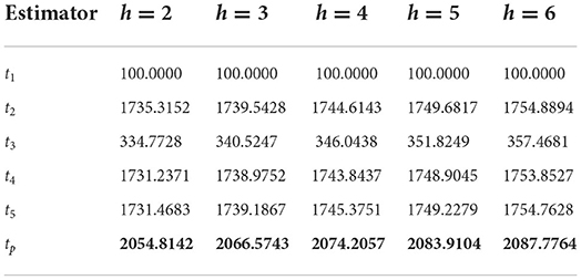
Table 7. PRE of different estimators with respect to t₁ for Population 6.

TABLE 8

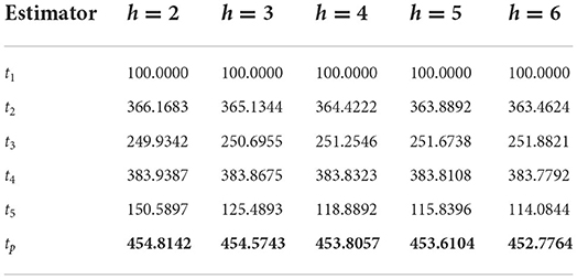
Table 8. PRE of different estimators with respect to t₁ for Population 7.

TABLE 9

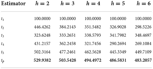
Table 9. PRE of different estimators with respect to t₁ for the simulated population.

Conclusion

We introduced a naive family of estimators for more efficient estimation of Ȳ using known auxiliary parameters in the case of nonresponse on both Yand X in the current study. For the approximation till order one, the bias and MSE of the introduced estimator were investigated. The optimum values of the characterizing scalars and the minimum value of the MSE of the introduced estimator were determined. The proposed estimator was theoretically compared to competing population mean estimators, and the efficiency criteria for the proposed estimator over competing estimators were determined. These efficiency criteria are verified using the five natural populations and one simulated population under investigation. The presented estimator is proven to be the most efficient estimator when compared to the class of competing estimators Hansen and Hurwitz [1], Khare and Kumar [40], Searls [39], and Unal and Kadilar [27], as it has the least MSE among these competing estimators for all seven real-world natural and one simulated data sets. As a result, the recommended estimators can be used in a variety of fields, such as Agricultural Science, Biological Sciences, Business, Commerce, Economics, Engineering, Fisheries, Mathematical Sciences, Medical Sciences, Poultry, and Social Sciences, in the case of nonresponse.

Data availability statement

The original contributions presented in the study are included in the article/supplementary material, further inquiries can be directed to the corresponding authors.

Author contributions

All authors listed have made a substantial, direct, and intellectual contribution to the work and approved it for publication.

Acknowledgments

The authors express their heartfelt thanks to the Associate Editor and the learned referees for their valuable comments which improved the earlier draft. The authors are also thankful to the Deanship of Scientific Research, Qassim University for funding the publication of this project.

Conflict of interest

The authors declare that the research was conducted in the absence of any commercial or financial relationships that could be construed as a potential conflict of interest.

Publisher's note

All claims expressed in this article are solely those of the authors and do not necessarily represent those of their affiliated organizations, or those of the publisher, the editors and the reviewers. Any product that may be evaluated in this article, or claim that may be made by its manufacturer, is not guaranteed or endorsed by the publisher.

References

1. Hansen MH, Hurwitz WN. The problem of non-response in sample surveys. J Am Stat Assoc. (1946) 41:517–29. doi: 10.1080/01621459.1946.10501894

PubMed Abstract | CrossRef Full Text | Google Scholar

2. El-Badry MA. A sampling procedure for mailed questionnaires. J Am Stat Assoc. (1956) 51:209–27. doi: 10.1080/01621459.1956.10501321

CrossRef Full Text | Google Scholar

3. Rao SRS. Ratio estimation with sub sampling the non-respondents. Surv Methodol. (1986) 12:217–30.

4. Khare BB, Srivastava S. Study of conventional and alternative two phase sampling ratio, product and regression estimators in presence of nonresponse. Proc Natl Acad Sci India Sect. (1995) 65:195–204.

5. Khare BB, Srivastava S. Transformed ratio type estimators for the population mean in the presence of nonresponse. Commun Stat. (1997) 7:1779–91. doi: 10.1080/03610929708832012

CrossRef Full Text | Google Scholar

6. Tracy DS, Osahan SS. Random non-response on study variable versus on study as well as auxiliary variables. Statistica. (1994) 54:163–8.

Google Scholar

7. Singh HP, Kumar S. A regression approach to the estimation of the finite population mean in the presence of non-response Australian and New Zealand. J Statistics. (2008) 4:395–408. doi: 10.1111/j.1467-842X.2008.00525.x

CrossRef Full Text | Google Scholar

8. Kumar S, Bhougal S. Estimation of the population mean in presence of non-response. Commun Stat. (2011) 18:537–48. doi: 10.5351/CKSS.2011.18.4.537

PubMed Abstract | CrossRef Full Text | Google Scholar

9. Grover LK, Kaur P. A generalized class of ratio type exponential estimators of population mean under linear transformation of auxiliary variable. Commun Stat. (2014) 43:1552–74. doi: 10.1080/03610918.2012.736579

CrossRef Full Text | Google Scholar

10. Bii NK, Onyango CO. Odhiambo J. Estimating a finite population mean under random non response in two stage cluster sampling with replacement. J. Physics: Conference Series. (2018) 1132:012071. doi: 10.1088/1742-6596/1132/1/012071

CrossRef Full Text | Google Scholar

11. Sharma P, Pal SK. Estimation of population mean in presence of random non-response. J Stat Manag Syst. (2018) 21:1105–19. doi: 10.1080/09720510.2018.1478623

PubMed Abstract | CrossRef Full Text | Google Scholar

12. Muneer S, Shabbir J, Khalil A. A generalized exponential type estimator of population mean in the presence of non-response. Stat Transit. (2018) 19:259–76. doi: 10.21307/stattrans-2018-015

CrossRef Full Text | Google Scholar

13. Toutenburg H, Srivastava VK. Estimation of ratio of population means in survey sampling when some observations are missing. Metrika. (1998) 48:177–87. doi: 10.1007/PL00003973

CrossRef Full Text | Google Scholar

14. Toutenburg H, Srivastava VK. Efficient estimation of population mean using incomplete survey data on study and auxiliary characteristics. Statistica. (2003) 63:223–36.

Google Scholar

15. Khare BB, Sinha RR. Estimation of the ratio of the two population means using multi auxiliary characteristics in the presence of non-response. In: Statistical Techniques in Life Testing. Reliability, Sampling Theory and Quality Control. Warsaw: Główny Urza̧d Statystyczny (2007). p. 63–171.

16. Khare BB, Sinha RR. On the class of estimators for population mean using multi auxiliary characters in the presence of non-response. Stat Transit. (2009) 10:3–14. doi: 10.21307/stattrans-2019-025

CrossRef Full Text | Google Scholar

17. Srinath KP. Multiphase sampling in non-response problems. J Am Stat Assoc. (1971) 66:583–6. doi: 10.1080/01621459.1971.10482310

CrossRef Full Text | Google Scholar

18. Tabasum R, Khan IA. Double sampling for ratio estimator for the population mean in the presence of non-response. Assam Statistical Review. (2006) 20:73–83.

19. Singh HP, Kumar S, Kozak M. Improved estimation of finite population mean using sub-sampling to deal with non response in two phase sampling scheme. Commun Stat Theory Method. (2010) 39:791–802. doi: 10.1080/03610920902796056

CrossRef Full Text | Google Scholar

20. Shabbir J, Khan NS. On estimating the finite population mean using two auxiliary variables in two phase sampling in the presence of non response. Commun Stat Theory Method. (2013) 42:4127–45. doi: 10.1080/03610926.2011.643851

CrossRef Full Text | Google Scholar

21. Yadav DK, Devi MM, Yadav SK. Estimation of finite population mean using known coefficient of variation in the simultaneous presence of non-response and measurement errors under double sampling scheme. J Reliability Stat Stud. (2018) 11:51–66.

Google Scholar

22. Sud UC, Srivastava SK. Estimation of population mean in repeat surveys in the presence of measurement errors. J Indian Soc Agric Stat. (2000) 53:125–33.

23. Srivastava K. and Shalabh, Effect of measurement errors on the regression method of estimation in survey sampling. J Stat Res. (2001) 35:35–44.

Google Scholar

24. Kumar S, Bhougal S, Nataraja NS, Viswanathaiah M. Estimation of population mean in the presence of non-response and measurement error. Revista Colombiana de Estadistica. (2015) 38:145–61. doi: 10.15446/rce.v38n1.48807

PubMed Abstract | CrossRef Full Text | Google Scholar

25. Kumar S. Improved estimation of population mean in presence of nonresponse and measurement error. J Stat Theory Pract. (2016) 10:707–20. doi: 10.1080/15598608.2016.1216488

CrossRef Full Text | Google Scholar

26. Singh P, Singh R, Bouza CN. Effect of measurement error and non-response on estimation of population mean. Revista Investigacion Operacional. (2018) 39:108–20.

Google Scholar

27. Unal C, Kadilar C. Adapted exponential type estimator in the presence of non-response. J Reliability Stat Stud. (2021) 14:311–22. doi: 10.13052/jrss0974-8024.14115

CrossRef Full Text | Google Scholar

28. Yadav SK, Yadav OP, Yadav DK. Dexterous estimation of population mean in survey sampling under non-response error. Int J Math Eng Manag Sci. (2019) 4:1307–27. doi: 10.33889/IJMEMS.2019.4.6-103

CrossRef Full Text | Google Scholar

29. Sharma V, Kumar S. Estimation of population mean using transformed auxiliary variable and non-response. Revista Investigacion Operacional. (2020) 41:438–44.

Google Scholar

30. Unal C, Kadilar C, A. New Family of exponential type estimators in the presence of non-response. J Math Fundam Sci. (2021) 53:1–15. doi: 10.5614/j.math.fund.sci.2021.53.1.1

CrossRef Full Text | Google Scholar

31. Unal C, Kadilar C, A. new population mean estimator under non-response cases. J Taibah Uni Sci. (2022) 16:111–9. doi: 10.1080/16583655.2022.2034343

CrossRef Full Text | Google Scholar

32. Jaiswal AK, Singh GN, Pandey AK. Improved procedures for mean estimation under non-response. Alexandria Eng J. (2022) 61:12813–28. doi: 10.1016/j.aej.2022.06.031

CrossRef Full Text | Google Scholar

33. Ahmed S, Shabbir J, Gupta S. Use of scrambled response model in estimating the finite population mean in presence of non response when coefficient of variation is known. Commun Stat Theory Method. (2017) 46:8435–49. doi: 10.1080/03610926.2016.1183782

CrossRef Full Text | Google Scholar

34. Yadav DK, Devi M, Yadav SK. Estimation of finite population mean using known coefficient of variation in the simultaneous presence of non-response and measurement errors under double sampling scheme. J Reliability Stat Stud. (2018) 11:51–66.

Google Scholar

35. Ahmed S. Shabbir J. Model based estimation of population total in presence of non-ignorable non-response. PLoS ONE. (2019) 14:e0222701. doi: 10.1371/journal.pone.0222701

PubMed Abstract | CrossRef Full Text | Google Scholar

36. Hussain S, Ahmad S, Akhtar S, Javed A, Yasmeen U. Estimation of finite population distribution function with dual use of auxiliary information under non-response. PLoS ONE. (2020) 15:e0243584. doi: 10.1371/journal.pone.0243584

PubMed Abstract | CrossRef Full Text | Google Scholar

37. Ahmad S, Hussain S, Aamir M, Khan F, Alshahrani MN, Alqawba M. Estimation of finite population mean using dual auxiliary variable for non-response using simple random sampling. AIMS Mathematics. (2022) 7:4592–613. doi: 10.3934/math.2022256

PubMed Abstract | CrossRef Full Text | Google Scholar

38. Singh R, Kumar M, Chaudhary MK, Smarandache F. Estimation of mean in presence of non-response using exponential estimator. arXiv. (2009) 0906.2462. doi: 10.48550/arXiv.0906.2462

CrossRef Full Text | Google Scholar

39. Searls DT. The utilization of a known coefficient of variation in the estimation procedure. J Am Stat Assoc. (1964) 59:1225–6. doi: 10.1080/01621459.1964.10480765

CrossRef Full Text | Google Scholar

40. Khare BB, Kumar S. Utilization of coefficient of variation in the estimation of population mean using auxiliary character in the presence of non-response. Natl Acad Sci Lett. (2009) 32:235–41.

41. Sinha RR, Kumar V. Estimation of mean using double sampling the non-respondents with known and unknown variance. Int J Comput Sci Math. (2015) 6:442–58. doi: 10.1504/IJCSM.2015.072963

CrossRef Full Text | Google Scholar

42. Khare BB, Srivastava S. Estimation of population mean using auxiliary character in presence of non-response. Natl Acad Sci Lett. (1993) 16:111–4.

43. Sinha RR, Kumar V. Families of estimators for finite population variance using auxiliary character under double sampling the non-respondents. Natl Acad Sci Lett. (2015) 38:501–5. doi: 10.1007/s40009-015-0380-6

CrossRef Full Text | Google Scholar

44. Satici E, Kadilar C. Ratio estimator for the population mean at the current occasion in the presence of non-response in successive sampling. Hacettepe J Math Stat. (2011) 40:115–24.

Google Scholar

45. Yadav SK, Dixit MK, Dhungana HN, Mishra SS. Improved estimators for estimating average yield using auxiliary variable. Int J Comput Sci Math. (2019) 4:1228–38. doi: 10.33889/IJMEMS.2019.4.5-097

CrossRef Full Text | Google Scholar