The soft computing FFNN method for adjusting heteroscedasticity on the time series model of currency exchange rate

1. Introduction

Financial data is important information related to the performance of the business. The record of all of the financial data is analyzed to monitor the performance and financial health in identifying how the fluctuation of the data. The fluctuations of the financial data are usually influenced by external factors. Consequently, the conditional variance of the financial data sets is getting greater or unstable and this is problematic for prediction. Return volatility is necessary for supporting the financial business and investor in decision-making in order to measure and control the risk in the market [1]. Therefore, the suitable models are expanded to estimate the currency exchange rates with some external factors in different countries [2].

The time series stationary model can be adjusted to its heteroscedasticity effect by building a suitable model of its time series residual. The results of the suitable time series model are expected to minimize the outlier of the data fluctuation so that the model building will approach the actual data. The suitable time series model for reducing the volatility of data can be solved with linear or nonlinear methods. It can be applied while forecasting the volatility of log-returns series in the energy market [3] and the price of wheat using maximum temperature at critical root initiation (CRI) stage as the exogenous variable in the agricultural commodity subject [4]. Two types of hybrid models Artificial Neural Networks (ANN) and Generalized Autoregressive Conditional Heteroscedasticity (GARCH) are compared regarding the residual model and information criteria. Thus, the results showed that the suitable time series model of the EGARCH-ANN model has better performance than other models because the EGARCH-ANN as a nonlinear model estimates the parameters using the numerical methods, which is more approaching the actual value than the linear method. As a linear method, the GARCH-type model has to fulfill some regression assumptions, especially the heteroscedastic error [5]. GARCH model is even combined with two or more methods, such as implied and realized volatility model to be the preferred model for predicting the volatility [6]. In advance, the GARCH model has several types that can be compared to estimate volatility for returns. For instance, the comparison between six types of GARCH models for estimating the Bitcoin return applies the replication study and the robustness analysis to determine whether the six GARCH-type models are appropriate for modeling the Bitcoin returns [7]. Thus, the nonlinear method of ANN as a valuable alternative is needed for neglecting the econometric specifications. In addition, the ANN method is applied for avoiding the nonlinearity in the conditional mean of time series and also improving the built model of ANN using the number of the finite testing sample [8]. Theoretically, the complex analysis of ANN reduces the dimensions of the feature set and turns the learning rate to help the networks recognize the new data so that the optimal parameters give better performance to predict the stock's trading price [9].

For further analysis of the volatility issue, the currency exchange rate as one of the crucial financial data is usually analyzed and modeled to know how the financial activities of the countries. The currency exchange rate of a country has a role in influencing changes in international trade and investment. The exchange rate is the price of a currency against other currencies. The exchange rate greatly influences the risk of profit or loss in a business activity carried out individually or in groups. Six currencies have stable value movements in international trade, namely the Japanese yen, Swiss franc, Canadian dollar, British pound, euro, and United States (US) dollar. As two major indexes of the US stock market in international trade, Nasdaq Composite and Dow Jones Industrial Average were also built their model to govern whether enhancements can be achieved by forecasting major stock indexes and their volatility incorporating the financial variables as a hybrid model [10].

Each country has a different policy regarding its currency exchange rate. Generally, there are three policies regarding currency exchange rates. First is the floating system, where the exchange rate of foreign currencies fluctuates without restraint by the demand and supply of currencies. The second one is a fixed exchange rate system, where this policy needs the intervention of the government to stabilize the fluctuation of the exchange rate led by changes in currency demand and supply. The third type is a controlled system between a floating and fixed exchange rate system. The exchange rate in this system is allowed to fluctuate against changes in demand and supply. It occurs because the intervention of the government has a stabilizing role in the exchange rate in the same periods to avoid short-term fluctuations in exchange rates. The international foreign exchange market has undergone significant changes since the gold standard was abolished in 1971. Before August 1971, the US dollar value was associated with a gold value of $ 35 per ounce, and the currency value of other countries was referred to as the value of the US dollar. In other words, world currencies are in a type of fixed exchange rate system. Since August 1971, the US dollar and other currencies have changed according to supply and demand. However, sometimes the United States and other countries intervene. Therefore, the United States currency policy can be described as a controlled exchange rate system.

In Indonesia, the volatility of the United States (US) dollar exchange rate against the Indonesia (ID) rupiah can affect investment by making stock prices unstable. This condition causes investors not to invest their capital, leading to a decline in stock prices. Prediction of the US dollar exchange rate against the ID rupiah is an alternative way to estimate future exchange rates. It can reduce the risk of loss due to the instability of the US dollar exchange rate against the ID rupiah. Thus, economic observers and investors can provide further action. Forecasting currency exchange rates with the classical time series model can be obtained using the classical method, namely the Autoregressive Integrated Moving Average (ARIMA). The model of ARIMA requires assumptions that have to be fulfilled, such as assumptions of normality, homoscedasticity, and non-autocorrelation. However, in real cases, not all assumptions can be fulfilled, so forecasting methods have been developed that do not require these assumptions. One of them is the Feed-Forward Neural Network method. The decision in combining the linear and nonlinear models is proposed to obtain a more accurate prediction model for various applications [11].

According to previous studies, several methods had been used to estimate the currency exchange rates. First, the ANN method was used for the British pound against the US Dollar [12]. The second one was the utilization of a hybrid model between ARIMA and ANN [13]. This model combines ARIMA and ANN models to see linear and nonlinear modeling of Wolf sunspot data, the distribution of lynx mammals in Canada, and the British pound was conducted. Experimental results from these data sets indicated that the combined model could be an effective way to improve the accuracy of forecasting models. Besides, the analysis of the model is needed to produce better forecasts than the classical model of time series [14]. Independent Component Analysis (ICA) is proposed to rebuild time series to be independent components as well as neural networks. The results showed that ICA extracts the noise of time series for having the explanatory variables so that it can improve the accuracy of forecasts. Furthermore, the accuracy of forecasts is also still depended on the stability of the training dynamics. The error of gradients for both different arrows of propagation, that are forward and backward, have a bearing on the stability of the networks [15].

In addition, to build a model of the exchange rate [16], the research predicted the daily period stock price index, namely NASDAQ, by using the Dynamic Artificial Neural Network (DAN2), combined models between neural networks and GARCH, and Multi-Layer Perceptron (MLP) method. They evaluated the effectiveness of the ANN model, which was known to be dynamic and effective in predicting stock prices. The prediction case of the exchange rate of the US Dollar against the Sri Lankan Rupee (USD/LKR) also showed that the ANN model performs better when compared with the GARCH model [17]. Each model was compared using the measurement accuracy of Mean Square Error and Mean Absolute Deviation. Stock price modeling was carried out by comparing ARIMA and ANN models in predicting Dell Technology's stock prices [18] where the ANN model had good accuracy compared to ARIMA. In international trade, the volatility of a stock's trading price can be analyzed by using the GARCH model to measure the financial risk [19].

For further analysis, the performance of the ARIMA-GARCH model is needed in modeling and forecasting the oil price [20]. This study estimated volatility in oil prices using static and dynamic forecasting. The results show that one-step forecasting provides better forecasting than finite-step forecasting. In modeling the Composite Stock Price Index, there are several factors that influence the Composite Stock Price Index, namely interest rates, inflation, crude oil prices, gold prices, and currency exchange rates. This study used the ANN model to build the Composite Stock Price Index modeling [21]. The research about neural networks was created again for analyzing the further application using ANN [22]. ANN is compared with nonparametric regression Multivariate Adaptive Regression Spline using the MAPE to determine the best model to build the model of Indonesian Composite Index with some internal factors such as interest rates, crude-oil prices, inflation, gold prices, exchange rates, Nikkei 225 Index, and Dow Jones price.

Based on the description of the previous research, forecasting conducted with the ANN method shows a pretty good result compared to other methods. Several studies compared ARIMA with ANN in that study and proposed modeling using the ARIMA-ANN model. The ANN model as the machine learning methodology applies soft computing to build a time series model. One type of ANN method processes the initial random weight with forwarding propagation to adjust the weights so that soft computing gives the best weights estimation in building the optimal fitted model of ANN. This soft computing will have larger iterations while the networks figure out the optimal weights with some initialization of networks, such as a smaller learning rate and a specific threshold value. This type is well-known as Feed-Forward Neural Networks (FFNN). Therefore, there is no accurate comparison between ARIMA-GARCH and ARIMA-FFNN. This study uses a soft computing method, that is FFNN, to adjust the heteroscedasticity of the time series model of ARIMA. To show this method has good performance in re-modifying the variance model using the accuracy measures of the model, the classical time series of GARCH is required as its comparison. Therefore, this study shows the accuracy model of the US dollar exchange rate against the ID rupiah using the ARIMA-GARCH, the ARIMA-FFNN, and the ARIMA-GARCH-FFNN model.

2. Materials and methods

2.1. Data source

This study uses a monthly period of the financial data of exchange rates between two countries, that are the United States and Indonesia. The source data can be accessed on the official website of Bank Indonesia, which is https://www.bi.go.id/. The exchange rate data of the US dollar against the ID rupiah select 245 data which started from January 2001 to May 2021.

2.2. The building of hybrid model of ARIMA-FFNN and ARIMA-GARCH-FFNN

Before the times series data {X_t} will be processed using a specific method, the data set has to be stationary. A stationary process makes the structure of data not change over time. If the time series data is non-stationary, the data will be chosen for the period under consideration. It makes the stationary of the time series so essential to change the structure of data to fluctuate around the mean and variance of the data set. It means that the stationary time series data set will therefore be in a particular episode, and it is impossible to change into the other time. However, in real-life problems, most of the data is not fluctuating around a value. Still, it can be changed over time because of many factors which influence the fluctuating data. It can be indicated as non-stationary data. Conversely, the non-stationary data can be improved to be stationary by using power transformation and differencing.

For detecting the stationarity of data, graph analysis can not be proposed to determine whether the time series data is already stationary, but it helps to know how the pattern of the data. The basic properties are still needed to determine the next decision. If the data have a constant mean and variance, the data is already stationary. If the variance of the data is non-stationary, it can be solved by using the power transformation, namely the Box-Cox transformation. Let T(X_t) is the transformation function of X_t. The following formula is used to stabilize the variance

$\begin{array}{ll}T(X_t)=\frac{X_t^{\lambda }-1}{\lambda }& (1)\end{array}$

for λ ≠ 0 and λ called transformation parameter. After the data is stationary in variance, it is followed by testing the stationary in the mean by using Augmented Dickey-Fuller (ADF) test. The random walk equation with drift for the differenced-lag model is regressed to be:

$\begin{array}{ll}\nabla X_t=\mu +\delta X_{t-1}+{\displaystyle \sum _{i=1}^k}{\varphi }_i\nabla X_{t-i}+e_t& (2)\end{array}$

for ∇X_t = X_t − X_t−1, k is the number of lags, δ is the slope coefficient, μ is a drift parameter, ϕ_i is parameter of random walk equation, and e_t is white noise error term. The test statistic is used as follows:

$\begin{array}{ll}ADF=\frac{\widehat{\delta }}{SE(\widehat{\delta })}& (3)\end{array}$

for $\widehat{\delta }$ as the estimated δ which is obtained by using ordinary least squares and $SE(\widehat{\delta })$ as the standard error of δ. The initial hypothesis is δ = 0, which means that the data is not stationary. The criteria for decision-making reject the initial hypothesis if the ADF value is less than the test statistics in the table.

In the real application of the study case, the sensitivity of data can be indicated by the fluctuation of the data that describes the non-random chaotic dynamics. The chaotic case leads to the linear model does not adequate to approach the extreme point. Therefore, the nonlinearity test is required to test the initial or null hypotheses of independent and identical distribution (iid). The Brock-Dechert-Scheinkman (BDS) test can be used to check the presence and detect the remaining dependence of omitted nonlinear structure. If the null hypothesis cannot be rejected, then the original linear model cannot be rejected, or if the probability values are less than the significant level so there are nonlinearity patterns in the dataset [23].

A time series {X_t} has the properties of white noise if a sequence of uncorrelated random variables with a specific distribution is identified by constant mean, usually assumed to be 0, a constant variance $Var(X_t)={\sigma }^2$ and Cov(X_t+h, X_t) = 0 for k ≠ 0. In time series analysis, there are some time series models such as ARIMA which is a combined two models between Autoregressive (AR) and Moving Average (MA) after differencing. The common form of the ARIMA model is expressed as follows:

$\begin{array}{ll}{\varphi }_p(B){(1-B)}^d{X}_t={\theta }_q(B){\epsilon }_t& (4)\end{array}$

with

$\begin{array}{l}{\varphi }_p(B)=(1-{\varphi }_{1}B-{\varphi }_2{B}^2-\cdots -{\varphi }_p{B}^p)\\ {\theta }_q(B)=(1-{\theta }_{1}B-{\theta }_2{B}^2-\cdots -{\theta }_q{B}^q)\end{array}$

where ϕ_p(B) is the Autoregressive components, θ_q(B) is the Moving Average components, B is the operator of backward shift, and ${(1-B)}^d{X}_t$ is stationary of time series in d-order differencing. This process is denoted by ARIMA(p,d,q).

After fitting the models, auto-correlation is used to diagnose the SARIMA residual as a linear relationship in dependency as follows:

$\begin{array}{ll}{Q}_{LB}=n(n+2){\displaystyle \sum _{i=1}^k}\frac{{\rho }_i^2}{n-i}& (5)\end{array}$

The number of observation data is denoted as n, ${\rho }_i^2$ is the sample auto-correlation coefficient at lag k = 1, 2, 3, …, K and K is lag length. The ARIMA residual is non-auto-correlation if $Q_{LB}>{\chi }_{\alpha }^2(k-p-q)$. In the normality test, Jarque Berra (JB) was used to diagnose ARIMA residuals whether or not they are normally distributed. The statistics test of JB is:

$\begin{array}{ll}JB=\frac{n}{6}(S^2\frac{{(K-3)}^2}{4})& (6)\end{array}$

where K and S are kurtosis and skewness, respectively. ARIMA residual will have normally distributed if $JB\le {\chi }_{\alpha }^2(2)$.

In the economic time series, the fluctuation of the data is usually influenced by four factors, such as trend, seasonal period, periodic factor or cycle, and also the irregular components. In 1982, Engle introduced the ARCH model and assumed that the variance of the data is influenced by the previous time. Based on the ARIMA model in Equation (4) and the variance assumption of the ARCH model, the ARCH(q) model can be written to be:

$\begin{array}{ll}{\sigma }_t^2={\alpha }_0+{\alpha }_1{\epsilon }_{t-1}^2+\cdots +{\alpha }_q{\epsilon }_{t-q}^2& (7)\end{array}$

where q presents the number of autoregressive terms in the model, ε_t denotes the ordinary least squares variance obtained from original regression model Equation (4), α_i is a parameter of ARCH model, ε_t = σ_te_t, and e_t ~ N(0, 1), α_i > 0 for i = 0, 1, 2, ⋯   , q.

In processing real data using ARCH, the model often has larger orders. It causes the estimated parameters are also getting larger. Therefore, the ARCH model is developed to be the preferred model, namely the GARCH model. As the concept of time series, the residual e_t is assumed to always be homoscedastic, i.e. $E(e_t^2)=E(e_t^2|e_{t-1}^2,e_{t-2}^2,\cdots )={\sigma }^2$ for every t. Whereas in the GARCH model, the e_t variance changes over time so that $E(e_t^2|e_{t-1}^2,e_{t-2}^2,\cdots )={\sigma }_t^2$ means the residual e_t is heteroscedasticity.

The GARCH model assumes that the initialed data has variances that always change over time. In other words, the fluctuations of the data are not fixed in the same value for each time t. In general, a GARCH(p,q) process is defined as a e_t process that satisfies:

$\begin{array}{ll}{\sigma }_t^2={\alpha }_0+{\displaystyle \sum _{i=1}^q}{\alpha }_i{\epsilon }_{t-i}^2+{\displaystyle \sum _{j=1}^p}{\beta }_j{\sigma }_{t-j}^2& (8)\end{array}$

where ε_t = σ_te_t, e_t ~ N(0, 1), q > 0, p ≥ 0, α_i ≥ 0, α₀ > 0, for i = 0, 1, 2, ⋯   , q and β_j ≥ 0 for j = 1, 2, ⋯   , p and also $\sum _{i=1}^q{\alpha }_i+\sum _{j=1}^p{\beta }_j<1$.

Then, the parameters of GARCH are firstly approximated by using the Maximum Likelihood Estimation (MLE) method. The residual of the ARIMA model is assumed to be white noise with a mean value of 0 and a variance of σ². After getting the log-likelihood function for n observed data, the parameters are estimated using the iteration processes, namely Newton Raphson. This method is used to find a solution to the probability log function. Thus, a sufficiently convergent value is obtained as an estimator for each parameter.

2.2.1. The building of ARIMA-FFNN model

After estimating the ARIMA model using Equation (4), the regression assumption of the ARIMA residual has to be fulfilled. Infrequently, there is the heteroscedasticity effect on the ARIMA residual so the ARIMA model which is obtained cannot be applied optimally to the actual data. Classically, this heteroscedasticity problem can be corrected using the GARCH model in Equation (8). However, as in the case of ARIMA, the GARCH residual has to fulfill the regression assumptions of autocorrelation, heteroscedasticity, and normality so that the GARCH residual is already distributed in white noise.

In this paper, the FFNN model is required as a comparison to adjust this heteroscedasticity problem. It is not only because the regression assumption of the GARCH residual can be ignored, but also because the structure of the FFNN model is almost similar to the GARCH model. Therefore, they are acceptable to be compared to each other. In contrast, the FFNN model has uniqueness in the network iteration. After the data is processed to the new units, the network is going to do the transformation using the activation function that is required to normalize the dataset into the proper range. Therefore, the output of each unit is always in the proper range. In other words, the estimated parameters of the FFNN model are stable or converge into the optimal value.

In forecasting, neural networks are also used to help predict a value in the future using numerical methods. Theoretically, the neural network is not only applied to adjust its weights but also led to improving the performance on real-world problems [24]. Based on the article on a logical calculus of the ideas immanent in nervous activities, McCulloch and Pitts explained how to construct an artificial neural network. The construction of the mathematical neuron model will be shown generally in Figure 1.

FIGURE 1

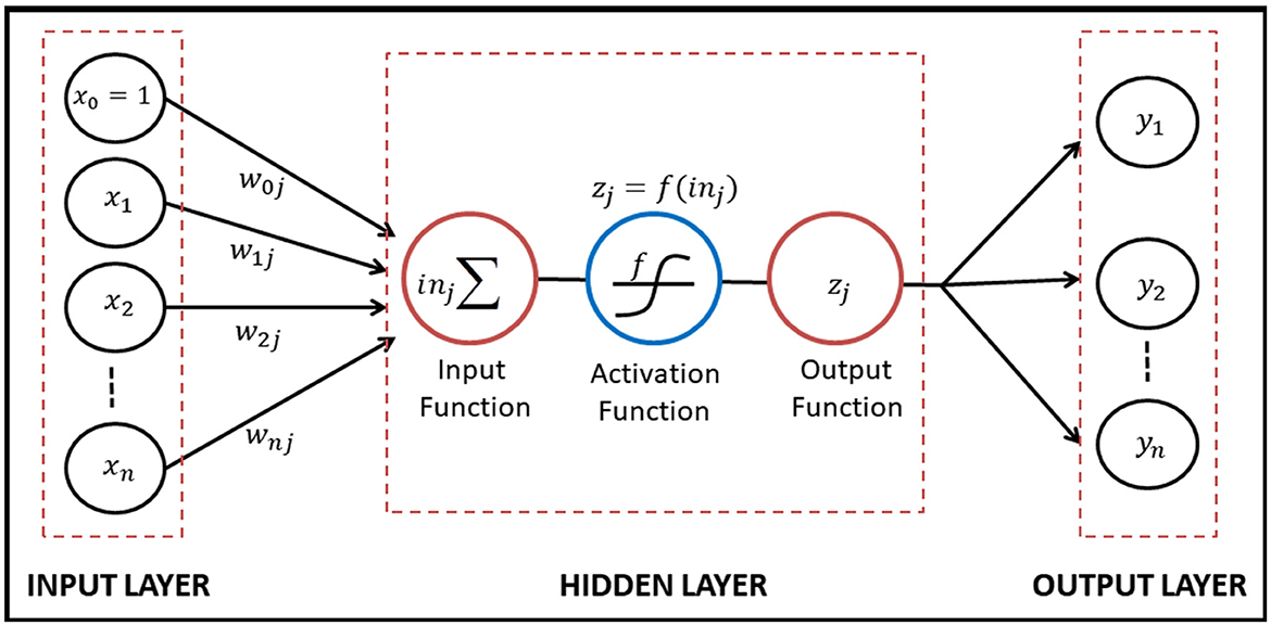
Figure 1. A construction of mathematical neuron model.

Based on Figure 1, artificial neural networks are formed by directed links that connect two or more units. The input layer accepted the independent variables as the input data of the model and it is denoted by x_i. A link from unit i to unit j has weight w_ij to determine the sign and strength of the input data. In the input function on the hidden layer, each unit j calculated a weighted sum of its inputs as follows:

$\begin{array}{ll}i{n}_j={\displaystyle \sum _{i=0}^n}{x}_i{w}_{ij}& (9)\end{array}$

Then the output z_j obtained by applying the activation function f so that $z_j=g(i{n}_j)=g(\sum _{i=0}^n{x}_i{w}_{ij})$ and the output z_j forwarded as the new input in the other neurons. The activation function f used to scale the output in Eq.(9) into proper ranges.

For transforming the results from one layer to another, there are three common activation functions provided in the neural network: linear, sigmoid, and hyperbolic tangent [25]. The function is chosen by the networks necessary. A linear function is the least commonly used between the activation functions because it does not transform the value into the proper range. A linear function is also discontinuous and hence will not suffice for the generalized delta rule. Thus, a continuous function provided nonlinear activation functions, which are sigmoid and hyperbolic tangents. In the sigmoid and hyperbolic tangent, there are upper and lower bounds. If the networks needed to return positive values, the sigmoid would be suitable because the function has a value between 0 and 1 which is associated with the proper range of the sigmoid function. The hyperbolic tangent function could not be provided because this function obtains positive and negative values.

After determining the mathematical model based on Figure 1, there are feed-forward and recurrent networks that are different in making the networks. In a feed-forward network, each input unit is received by the unit in the prior layer. The result is depended on the type of layers, which are single-layer and multilayer networks. In the multilayer network, there are one or more layers as a link between the input and output layers, namely hidden layers. Conversely, in the recurrent network, its outputs return to be its inputs in the previous layer. This network forms a dynamical system to approach the stable state so that the input depends on its initial value in prior inputs. It makes the network more approaching the brain but also more difficult to be learned.

Before getting the neural network model, the data is separated to be training and testing set data [25]. It helps the model to recognize the new data which will be entered into the model. In a training network, a neuron is interconnected through the output units to the other neurons. Each connection is associated with weight which is not always equal to the different weights in the same units. These initial weights will determine the output of the networks. Otherwise, the training network also depends on the output usage in the output layer. If the training network is given sample data with expected outputs from these data, the network uses supervised training proceeds. The model in this procedure is taken through the number of iterations or epochs, the network's output which matches with an anticipated output and the boundary value of error assessment.

Conversely, unsupervised training proceeds do not provide the anticipated output in training. It occurs when the network wants to classify the input data into several categories. There is also the other type of training proceed that are combining supervised and unsupervised proceeds. The network does not need the anticipated output, but the networks determine whether wrong or right the given input for each output is. A sample dataset of training networks using their anticipated output was used to predict the error of the network, which is substantially lower than the boundary value. After the networks are trained, it is essential that the performances of the network are measured by testing that is used in the learning stage. It finds out whether the network is able to make significant generalizations.

After the neural network model is obtained, the essential step to determining whether additional training is required or iteration has finished the validation of the model. Suppose the validation data is insufficient or input data was not available in the train of data. In that case, it can be solved with different random separating datasets into training and testing processes. If it is not working, one large training dataset needed to be combined with the old dataset. Then, the process can be repeated until the validation of the network is fulfilled.

In the training process, the error as the threshold limit is required to decide whether the iteration of the process will be repeated or stopped. This threshold limit is obtained based on the difference between the actual and estimated output which depends on the iteration. If there is no difference, no learning occurs, or the initial weight will be changed to reduce the error. In minimizing the square of the error as summed over the square of the differences between all output units and observational values, the gradient descent controlled by the delta rule provided to show the change of weight has the negative constant proportionality to the change of the error measure Err(W) with respect to each weight. The iteration of the process is repeated until a minimum error is reached. The change of the gradient of the error function Err(W) is denoted by ∇Err(W) and the change in all weights is denoted by ΔW. The relation between the change of every single weight and error function can be written as follows:

$\begin{array}{ll}\Delta w_{jt}=-\eta \frac{\partial Err(W)}{\partial w_{jt}}& (10)\end{array}$

where Err(W) is the error function, η is learning rate, w_jk is single weight between the jth hidden and the kth output unit layer. In general, the training networks modify the connection weights using the learning rate iteratively until the error between the outputs given by the estimated output is less than a specific threshold as explained in [25]. The gradient descent requires the infinitesimal steps to be selected to help reach the optimal single unit of weight in the training networks. Therefore, the infinitesimal steps need constant proportionality, that is the learning rate, to minimize the derivative of error measure for each weight in the gradient descent procedure. If the constant proportionality is larger, then the changes in the weight are getting larger. It means that the change of the weight for each train in the network is more rapid learning. But, it will not be stable and converge into a value. Then, the application of soft computing is necessary to use for random weight estimation.

The network trained with the feed-forward method started by initialization of the network, which consists of the initial random value of weights, building architecture of the network, and determining the constant value of the learning rate. Then, process the input data using a feed-forward network: the associated weights and input layer is transformed using the preferred activation function and passed forward to the hidden and output layer through the network. After the estimated output of the trained network is obtained, the estimated output has to be compared with the actual value of output until getting the error. If the trained error is less than a specified threshold, then the network is passed forward to the validation process and the network's algorithm is terminated. Conversely, if the error is greater than a threshold value, the network has to propagate the error. It means that the error will be used to re-modify the previous weights and to compute the change of gradient in error for changes in the weight values. Finally, the network adjusts the old weights using the change of gradient to minimize the error.

The training process is proposed to adjust the old weights using the change of gradient. It means that the networks attempt to minimize the error. The error for each k-th training data is defined as follows:

$\begin{array}{ll}Er{r}_k(W)=\frac{1}{2}{\displaystyle \sum _{j=1}^Q}{(t_{kj}-y_{kj})}^2& (11)\end{array}$

where Q is the number of output units, t_kj is actual data in j-th output unit layer, and y_kj is the training output in j-th output unit layer. The total error of weights W can be expressed as follows:

$\begin{array}{ll}Err(W)={\displaystyle \sum _{k=1}^m}Er{r}_k(W)& (12)\end{array}$

for kth training output data and m as the number of the training output data. An input vector is defined as ${\text{x}}_k={(x_{k1},x_{k2},\dots ,x_{kN})}^T$ in input layer of the networks. The input layer distributes its input units into every unit in the hidden layer as follows:

$\begin{array}{ll}i{n}_{kp}^h={\displaystyle \sum _{i=1}^N}{w}_{pi}^h{x}_{ki}+w_{p0}^h& (13)\end{array}$

where $w_{pi}^h$ as the weight between ith input unit and pth hidden unit, w_p0 as the bias, and h as the hidden layer. Assume that the activation function of the unit layer associated with the hidden layer is denoted as $f_p^h$. Therefore, the new value for each unit in the hidden layer is calculated as follows:

$\begin{array}{ll}{i}_{kp}=f_p^h(i{n}_{kp}^h)& (14)\end{array}$

The hidden layer distributes its hidden units into every unit in the output layer to obtain in_kj and then transforms the value of in_kj using the activation function $f_j^o$ in the output layer as follows:

$\begin{array}{ll}i{n}_{kj}^o={\displaystyle \sum _{p=1}^L}{w}_{jp}^o{i}_{kp}+w_{j0}^o& (15)\end{array}$

$\begin{array}{ll}{y}_{kj}=f_j^o(i{n}_{kj}^o)& (16)\end{array}$

where o as the representative of output layer, $w_{jp}^o$ as the weight pth hidden unit which is associated to jth output unit, and $w_{j0}^o$ as the bias.

Let the error of j single output unit in kth training data is denoted as δ_kj = (t_kj − y_kj), where t_kj is the observational or actual data and y_kj is the j output data in training networks. The adjustment of the weights can be processed in the hidden and output layers.

1. Adjust the weights in the output layer.

The error function of the weights in the hidden layer associated with the output layer is obtained by using the partial derivative as follows:

$\begin{array}{l}Er{r}_k(W)=\frac{1}{2}{\displaystyle \sum _{j=1}^Q}{(t_{kj}-y_{kj})}^2\end{array}$

$\begin{array}{ll}\frac{\partial Er{r}_k(W)}{\partial w_{jp}^o}=-(t_{kj}-y_{kj})\frac{\partial f_j^o}{\partial i{n}_{kj}^o}\frac{\partial i{n}_{kj}^o}{\partial w_{jp}^o}& (17)\end{array}$

where Q is the number of output units. Then substitute the value of $i{n}_{kj}^o$ in the Equation (15) to $\frac{\partial i{n}_{kj}^o}{\partial w_{jp}^o}$ so we have

$\begin{array}{ll}\frac{\partial i{n}_{kj}^o}{\partial w_{jp}^o}=\frac{\partial }{\partial w_{jp}^o}({\displaystyle \sum _{j=1}^L}{w}_{jp}^o{i}_{kp}+w_{j0}^o)=i_{kp}& (18)\end{array}$

Therefore, Equation (17) can be replaced to be

$\begin{array}{ll}-\frac{\partial Er{r}_k(W)}{\partial w_{jp}^o}={\delta }_{kj}^o{i}_{kp}& (19)\end{array}$

In substituting Equation (19) into Equation (10), the weights of the output layer can be obtained as follows:

$\begin{array}{ll}{w}_{jp}^o(t+1)=w_{jp}^o(t)+{\Delta }_k{w}_{jp}^o(t)& (20)\end{array}$

where

$\begin{array}{ll}{\Delta }_k{w}_{jp}^o=\eta (t_{kj}-y_{kj})f_j^{{}^{\prime }o}(i{n}_{kj}^o)i_{kp}& (21)\end{array}$

$\begin{array}{ll}{\delta }_{kj}^o=(t_{kj}-y_{kj})f_j^{{}^{\prime }o}(i{n}_{kj}^o)& (22)\end{array}$

2. Adjust the weights in the hidden layer.

Based on Equation (11), Err_k(W) can be described as follows:

$\begin{array}{l}Er{r}_k(W)=\frac{1}{2}{\displaystyle \sum _{j=1}^Q}{(t_{kj}-y_{kj})}^2=\frac{1}{2}{\displaystyle \sum _{j=1}^Q}{(t_{kj}-f_j^o({\displaystyle \sum _{p=1}^L}{w}_{jp}^o{i}_{kp}+w_{j0}^o))}^2\end{array}$

The gradient of Err_k(W) is obtained by using the partial derivative with respect to the weight of the input layer associated with the hidden layer $w_{pi}^h$ so we have

$\begin{array}{l}Er{r}_k(W)=\frac{1}{2}{\displaystyle \sum _{j=1}^Q}{(t_{kj}-y_{kj})}^2\end{array}$

$\begin{array}{ll}\frac{\partial Er{r}_k(W)}{\partial w_{pi}^h}=-{\displaystyle \sum _{j=1}^Q}(t_{kj}-y_{kj})\frac{\partial y_{kj}}{\partial i{n}_{kj}^o}\frac{\partial i{n}_{kj}^o}{\partial i_{kp}}\frac{\partial i_{kp}}{\partial i{n}_{kp}^h}\frac{\partial i{n}_{kp}^h}{\partial w_{pi}^h}& (23)\end{array}$

$\begin{array}{ll}\frac{\partial Er{r}_k(W)}{\partial w_{pi}^h}=-{\displaystyle \sum _{j=1}^Q}(t_{kj}-y_{kj})f_j^{o^{\prime }}(i{n}_{kj}^o)w_{jp}^o{f}_p^{h^{\prime }}(i{n}_{kp}^h)x_{ki}& (24)\end{array}$

By substituting the Equation (24) into Equation (10), the change of weight in the hidden layer can be calculated as follows:

$\begin{array}{ll}{\Delta }_k{w}_{pi}^h=\eta f_p^{h^{\prime }}(i{n}_{kp}^h)x_{ki}{\displaystyle \sum _{j=1}^Q}(t_{kj}-y_{kj})f_j^{o^{\prime }}(i{n}_{kj}^o)w_{jp}^o& (25)\end{array}$

$\begin{array}{ll}{\Delta }_k{w}_{pi}^h=\eta f_p^{h^{\prime }}(i{n}_{kp}^h)x_{ki}{\displaystyle \sum _{j=1}^Q}{\delta }_{kj}^o{w}_{jp}^o& (26)\end{array}$

Therefore, the adjustment of weights in the hidden layer can be expressed as follows:

$\begin{array}{l}{w}_{pi}^h(t+1)=w_{pi}^h(t)+{\Delta }_k{w}_{pi}^h=w_{pi}^h(t)+\eta {\delta }_{kp}^h{x}_{ki}\end{array}$

where the value of ${\Delta }_k{w}_{pi}^h$ is obtained by substituting the Equation (26) and

$\begin{array}{ll}{\delta }_{kp}^h=f_p^{h^{\prime }}(i{n}_{kp}^h){\displaystyle \sum _{j=1}^Q}{\delta }_{kj}^o{w}_{jp}^o& (27)\end{array}$

The adjustment of weights can be used for readjusting the weights of the networks which have not fulfilled the stop criterion in training processing. After terminating the training processing, the adjustment of the weights will be substituted to the preferred FFNN model, and it can be applied to adjust the heteroscedasticity of the time series model.

2.2.2. The building of ARIMA-GARCH-FFNN model

After building the ARIMA model and adjusting the heteroscedasticity effects using the GARCH model, this ARIMA-GARCH model is then continued to be combined with FFNN to determine whether this new proposed model of ARIMA-GARCH-FFNN is better performance than ARIMA-GARCH. The hybrid of the ARIMA-GARCH-FFNN model is obtained by combining the algorithms of ARIMA, GARCH, dan FFNN in Equations (4), (8), and (16), respectively.

2.3. Measures accuracy and goodness of fit

After the proposed model is obtained, the model will be evaluated the performance based on the fit of the forecasting or time series to historical data. There are many statistical measures to describe how well a model fits a given sample of data. The measuring accuracy should always be evaluated as part of a model validation effort. When more than one technique of model seems reasonable for a particular application, these accuracy measurements can also be used to discriminate between competing models.

In this research, there are two measures of model accuracy are used. First, Mean Absolute Percentage Error (MAPE) is applied to measure the model's accuracy using particular methods in a given observational data set. MAPE can be calculated as follows:

$\begin{array}{ll}MAPE=\frac{1}{N}{\displaystyle \sum _{t=1}^N}\frac{|Y_t-\widehat{Y_t}|}{Y_t}\times 100& (28)\end{array}$

Second, Mean Square Error (MSE) is applied to measure the average error of a model. MSE can be calculated as follows:

$\begin{array}{ll}MSE=\frac{SSE}{N}=\frac{{\displaystyle \sum _{t=1}^N}{(Y_t-\widehat{Y_t})}^2}{N}& (29)\end{array}$

where SSE is the sum of squared errors, N is the number of data set, y_i is the actual output data, and $\widehat{Y_t}$ is the estimated output using a certain forecasting method.

In fitting the ARIMA model, first, determine the order of the ARIMA model, estimate unknown parameters, and collect model candidates with a p-value of less than the significance level, carrying out regression assumption of the estimated residuals; and forecasting the future values using the known data. The fitting of ARIMA models requires the use of autocorrelation function charts. If the candidate model has been selected, then the best model selection is based on the AIC and BC values. Systematically the equations of AIC and BIC can be written respectively as the following:

$\begin{array}{ll}AIC=nln({\widehat{{\sigma }_{\epsilon }}}^2)+2k& (30)\end{array}$

$\begin{array}{ll}BIC=nln({\widehat{{\sigma }_{\epsilon }}}^2)+kln(n)& (31)\end{array}$

for n is the number of observations, ${\widehat{\sigma }}_{\epsilon }^2$ is the maximum likelihood estimator of ${\sigma }_{\epsilon }^2$, and k is the number of parameters estimated. The best model is the model that has the smallest value of AIC and BIC.

In determining whether there is a significant difference between the two models or having better predictive accuracy, the Diebold-Mariano test is required. The two forecasted model is selected and then compared in their error measurement using the statistic test of Diebold-Mariano as follows [26]:

$\begin{array}{ll}DM=\frac{\overline{d}}{\sqrt{({\gamma }_0+2{\displaystyle {\sum }_{k=1}^{h-1}{\gamma }_k}})/n}& (32)\end{array}$

where $\bar{d}$ represents the mean of the difference between two squared errors or loss-differential, γ_k represents the autocovariance at lag k, and n is the number of observational data.

After estimating the best model, the ratio of sums of squares of regression (SSR) to the sums of squares total (SST) can be compared to obtain the coefficient determination R². This measurement has the range on the closed interval [0, 1]. If the value of R² approaches the lowest value of 0, then it indicates a poor fit for the estimated model. In contrast, if the value of R² approaches the highest value of 1, then it indicates well fit for the estimated model. Let ȳ is defined as the mean of data set y_i, i = 1, 2, ⋯   , n so the R² can be calculated as follows:

$\begin{array}{ll}{R}^2=\frac{{\displaystyle {\sum }_{i=1}^n}{(y_i^{\prime }-ȳ)}^2}{{\displaystyle {\sum }_{i=1}^n}{(y_i-ȳ)}^2}& (33)\end{array}$

The value of R² is defined as the proportion of variance in the response variable accounted for by knowledge of the predictor variable(s). R² is also simultaneously the squared correlation between observed values on y_i and predicted values $y_i^{\prime }$ based on the data processing [27].

3. Data processing to adjust the heteroscedasticity effects

This study uses a monthly period of the financial data of exchange rates between two countries, that are the United States and Indonesia. The exchange rate data of the US dollar against the ID rupiah select 245 data which started from January 2001 to May 2021.

3.1. The classical model of ARIMA-GARCH for exchange rate

Firstly, we have to know how the fluctuation of the data will be used. The plotting of the exchange rate of the US dollar - ID rupiah can be displayed in Figure 2.

FIGURE 2

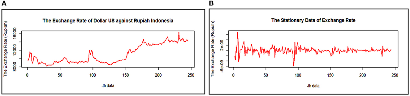
Figure 2. The exchange rate of the US dollar-ID rupiah of (A). Actual data and (B). Stationary data.

Based on Figure 2A, the variance of the data seems to change over time so that the data is not stationary against the variance. In order to produce the variance of the observational data to be stationary, Box-Cox transformation is purposed to minimize the fluctuation of the data. The Box-Cox transformation results give the parameter's value of λ is −1.6768 and 1. It expresses that the data will be transformed once to get the new data. At the same time, the plotting data shows that it has a trend so the dataset should fluctuate in around the mean. It is also reinforced by the results of the ADF test with a p-value of 0.2310, which is greater than the significance level of 0.05 and displayed in the following Table 1.

TABLE 1

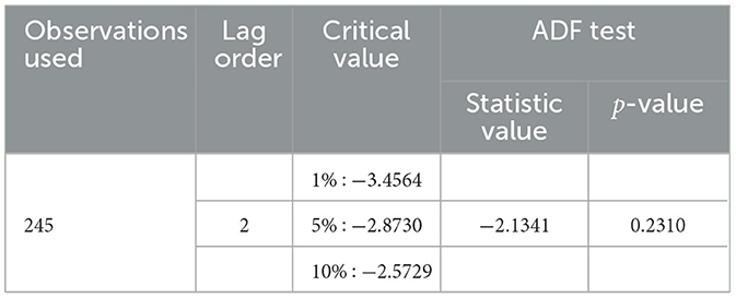
Table 1. Augmented Dickey–Fuller test.

Based on Table 1, the observational dataset of 245 has the optimum lag order of 2, where this optimal value is obtained based on the smallest value of AIC. The results of the ADF test indicate that the mean of the data is not stationary yet. Furthermore, the exchange rate data has to make a difference. The stationary data using the ADF test and Box-Cox transformation is shown in Figure 2B.

The presence of the nonlinearity pattern in the dataset can be checked by using the Brock-Dechert-Scheinkman (BDS) test. The result of BDS test in Table 2 shows that all the probability values are lower than the significant level of 5%. It means that all the exchange rates of the US dollar - ID rupiah series have a nonlinear pattern.

TABLE 2

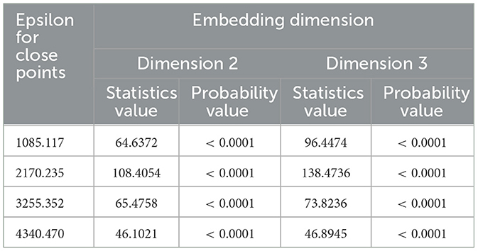
Table 2. BDS test results.

After the data are already stationary, the order p and q of the model can be obtained using the ACF and PACF chart. Figure 3 below shows the ACF and PACF chart for determining the order p and q of the ARIMA model.

FIGURE 3

Figure 3. The chart of (A) Auto-Correlation Function (ACF) and (B) Partial Auto-Correlation Function (PACF) for determining the order of ARIMA model.

Based on Figure 3, the ACF chart shows that the cut-off data movement after lag 2 and is assumed to be the order of MA q = 2 and the PACF chart shows that the cut-off data movement after lag 2, so AR order is suspected p = 2. Because the data is stationary, it is assumed that the initial conjecture model formed is the ARIMA(2,1,2). After estimating the parameters model in some possible models using the combination of the order of the ACF and PACF chart, the significant parameters of the model are determined using the p-value, which is lower than the significance level of 0.05. The significant parameters among the combination of the ACF and PACF chart order that is possible to build the ARIMA model are ARIMA(1,1,2) and ARIMA(2,1,1). Their estimation parameters can be shown in the following Table 3.

TABLE 3

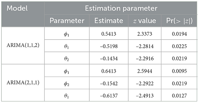
Table 3. Estimation significant parameters of ARIMA model.

Then, the most important step in the classical time series method is the regression assumptions of normality, homoscedasticity, and auto-correlation for the residual possible ARIMA model in Table 3. The following Table 4 represents that the p-value for the regression assumption of the residual ARIMA(1,1,2) and ARIMA(2,1,1).

TABLE 4

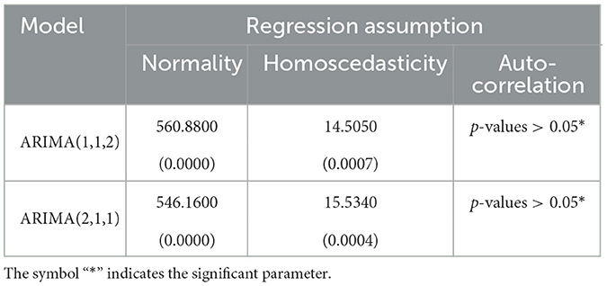
Table 4. Residual diagnosis checking for possible ARIMA model.

Based on Table 4, the residual of ARIMA(1,1,2) and ARIMA(2,1,1) contain the heteroscedasticity effect, non-auto-correlation and non-normally distributed. Although the data are not normally distributed, this model is still suitable since this is often occurred with the economic data due to fluctuating movements. Before solving the heteroscedasticity effect of the residuals ARIMA model, the possible ARIMA model can be chosen by using the Akaike or Bayesian Information Criterion as displayed in the following Table 5.

TABLE 5

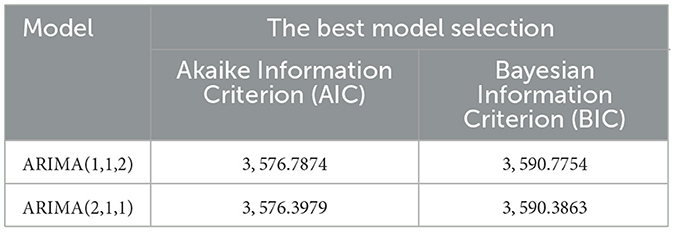
Table 5. Comparison of the possible ARIMA models.

The preferred model is selected regarding the smallest value of BIC or AIC. Based on Table 5, ARIMA(2,1,1) has the smallest value of AIC and BIC among the other possible ARIMA models. Therefore, ARIMA(2,1,1) model can be applied in the next step to break the effect of heteroscedasticity by repairing its variance of the residual model. The ARIMA(2,1,1) model can be written as follows:

$\begin{array}{cc}{\varphi }_1(B)(1-B)X_t={\theta }_2(B){\epsilon }_t& (34)\end{array}$

with ϕ_p(B) = (1 + 0.6137B) and ${\theta }_2(B)=(1-0.6413B+0.1542B^2)$.

After getting the fitted ARIMA(2,1,1) model, graphically, it can be analyzed to illustrate how its actual data is associated to its residual and fitted ARIMA(2,1,1) model in Figures 4A, B, respectively, as shown as in the following Figure 4.

FIGURE 4

Figure 4. The actual data point with (A) fitted ARIMA (2,1,1) data and (B) residual ARIMA (2,1,1) data.

The forecasting accuracy of the fitted ARIMA model is more closely approaching the actual data if the set of points between actual and fitted data forms a straight line y = x. Based on Figure 4A, it shows that the trend of the points set, which is established by the actual and fitted data, has formed a straight line y = x. It means that the fitted ARIMA(2,1,1) model almost approaches the actual data. Therefore, it can be concluded that the fitted ARIMA(2,1,1) model has been good enough to model the exchange rate US dollar against the ID rupiah.

The relationship between the values of the residual term is one of the regression assumptions that have to be fulfilled, namely non-auto-correlation. The residual data does not have the auto-correlation effect if the positive and negative error values are random. During the same period, if the fitted model almost approaches the actual data, then the residual of the fitted data will be getting smaller and even closer to zero. Based on Figure 4B, the residual of the fitted data has distributed around zero, and it doesn't form a pattern. In other words, the residual of the fitted ARIMA(2,1,1) model has been randomly distributed around zero. It also has fulfilled the regression assumption of non-auto-correlation.

After obtaining the Autoregressive Integrated Moving Average Model, there is a heteroscedasticity effect in the residual ARIMA model so the advanced model for adjusting the model is required. The following subsections describe three alternative methods that can be applied to solve the heteroscedasticity effects, such as GARCH, FFNN, and models of GARCH-FFNN.

The GARCH model is one of the methods which can be used to improve the classical model for getting the smallest variance in the residuals of the ARIMA model. The order of the GARCH model was obtained using ACF and PACF charts. The following Figure 5 shows ACF and PACF charts for the GARCH model.

FIGURE 5

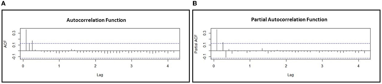
Figure 5. The chart of (A) auto-correlation function (ACF) and (B) partial auto-correlation function (PACF) for determining the order of GARCH model.

Based on Figure 5, it shows that ACF and PACF charts are significant in lag 3. Furthermore, the initial conjecture models for orders P and Q are the combinations of 0, 1, 2, and 3. After estimating the parameters model in some possible models using the combination of the order of the ACF and PACF chart, the significant parameters of the model are determined using the p-value, which is lower than the significance level. The significant parameters among the combination of the order of the ACF and PACF chart that is possible to build the GARCH model are GARCH(1,0), GARCH(1,1), and GARCH(2,0). Their estimation parameters of the GARCH model with the value of AIC or BIC can be shown in the following Table 6.

TABLE 6

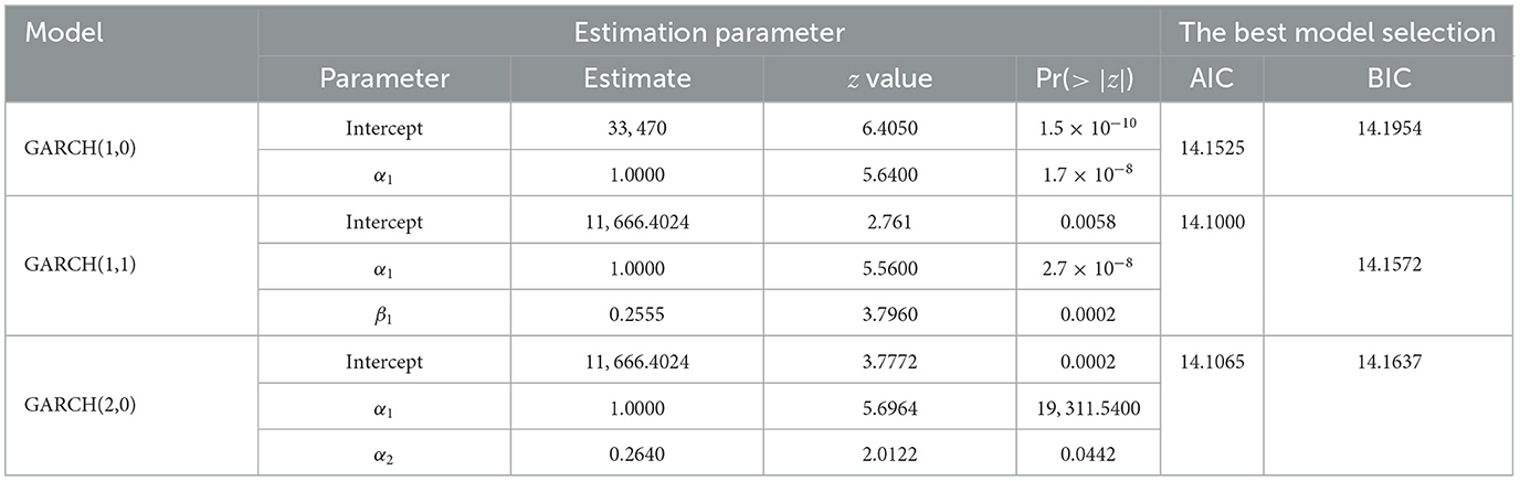
Table 6. Estimation of significant parameters of the GARCH model with their AIC or BIC value.

The best model is selected by using the smallest value of AIC or BIC. Based on Table 6, GARCH(1,1) has a smaller value AIC and BIC than the other possible models. Therefore, GARCH(1,1) model is the best model to improve the residual estimation of the ARIMA(2,1,1) model. The residual model of GARCH(1,1) can be written to be:

$\begin{array}{cc}{\sigma }_t^2=11666.4024+{\epsilon }_{t-1}^2+0.2555{\sigma }_{t-1}^2+{ϵ}_t^{*}& (35)\end{array}$

where ε_t = σ_te_t, e_t ~ N(0, 1), and ${ϵ}_t^{*}$ as the residual of the GARCH model. By combining the ARIMA and GARCH models, this new model of ARIMA(2,1,1)-GARCH(1,1) can be one of the alternatives to do forecasting the exchange rate value US dollar against the ID rupiah in the future.

3.2. Hybrid model of ARIMA-FFNN for exchange rate

As in the previous research [28], the exchange rate change among some currencies against US Dollar applies the time series Multilayer Perceptron (MLP) models in order to predict exchange rate change among Turkish, American, and European currencies. Thus, in determining the FFNN model by applying soft computing for the case of the exchange rates US Dollar - ID Rupiah, firstly, the input and output data are determined. Input data used are the residual of the ARIMA(2,1,1) model of the exchange rate US dollar against the ID rupiah. It can be determined by using the ACF and PACF chart so that the input data are obtained by the first, second, and third lag, or inputs data can be denoted as the (t − 1)-th, (t − 2)-th and (t − 3)-th data, respectively. At the same time, the target data is denoted by the t-th data. The second one is the standardization of the data. All observational data have to transform into a proper interval of numbers between 0 and 1 because it depends on the sigmoid's activation function used in networks. Then, the feed-forward neural network architecture will be constructed to know how many units for each layer are. Based on the data, the feed-forward neural network architecture applied is 3 − 4 − 2 − 1. The networks consist of three input units, four units in the first hidden layer, two units in the second hidden layer, and one output unit.

The process of the dataset is continuing for training the network. The next step is the learning algorithm of the feed-forward neural networks, it consists of the initialization of the instruments of networks, feed-forward of the networks, error evaluation, backpropagation, and adjustment of single weight. In the initialization of the network, the network is usually generated by random weights. In the training process, the instruments use 182 data as input units and the sigmoid function as the activation function between two layers. The gradient descent procedure uses the learning rate (η) of 0.01 while repeating the training process until the algorithm is stopped based on the threshold limit of 0.001. In feed-forward, each input unit (x_ki, i = 1, 2, 3) receives input observational data and propagates the summed results between the data and its associated weight into each hidden unit. Then, the stopping criterion is available if the error evaluation has the difference between observed output and training output is less than 0.001. In backpropagation, the correction value of weights and bias are used to make the error lower than 0.001. The new weight will be obtained in the adjustment process, from feed-forward until the adjustment process will be repeated if the error has not obtained lower than 0.01.

The fifth step is the validation of the network. For 182 data of training and 60 data of testing, the sample of training and testing data will be compared to determine whether the iteration of the network processes will be continued or stopped. The result of the validation can be shown in Table 7.

TABLE 7

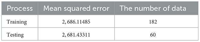
Table 7. Iteration summary for training and testing process.

Based on Table 7, the result shows that the Mean Squared Error (MSE) value of the training process is greater than the testing process. It indicates that feed-forward neural networks have the capability in recognizing new data. Therefore, the training process can be terminated and the optimal weights of neural networks can be applied to build a nonlinear model of residual ARIMA. After repeating the iteration processes, the input units of the first (X_t−1), second (X_t−2), and third (X_t−3) lags of the residuals of ARIMA(2,1,1) with four units in the first hidden layer and two units in the second hidden layer are applied to build the architecture of the FFNN model that will be shown in Figure 6.

FIGURE 6

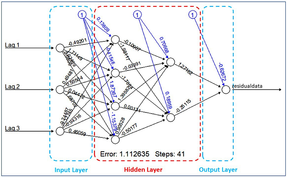
Figure 6. Architecture 3 − 4 − 2 − 1 of FFNN model with their weights for each unit.

For detail, the parameter estimation for each unit of the layers as the result of the iteration will be explained in two following Tables 8, 9.

TABLE 8

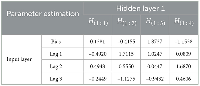
Table 8. Parameter estimation of FFNN model from input layer to hidden layer 1.

TABLE 9

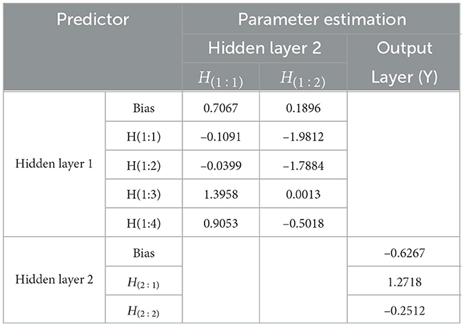
Table 9. Parameter estimation of FFNN model from hidden layer to output layer.

Based on Tables 8, 9 hidden layer 1 model of FFNN(3,4,2,1) can be written to be:

$\begin{array}{l}{H}_{(1:1)}=f_p^{h1}(w_{10}^{h1}+{\displaystyle \sum _{i=1}^3{x}_{ti}}{w}_{1i}^{h1})=f_p^{h1}(0.1381\\ -0.4920x_{t1}+0.4948x_{t2}-0.2449x_{t3})\\ H_{(1:2)}=f_p^{h1}(w_{20}^{h1}+{\displaystyle \sum _{i=1}^3{x}_{ti}}{w}_{2i}^{h1})=f_p^{h1}(-0.4155\\ +1.7115x_{t1}+0.5550x_{t2}-1.1275x_{t3})\\ H_{(1:3)}=f_p^{h1}(w_{30}^{h1}+{\displaystyle \sum _{i=1}^3{x}_{ti}}{w}_{3i}^{h1})=f_p^{h1}(1.8737\\ +1.0247x_{t1}+0.0447x_{t2}-0.9432x_{t3})\\ H_{(1:4)}=f_p^{h1}(w_{40}^{h1}+{\displaystyle \sum _{i=1}^3{x}_{ti}}{w}_{4i}^{h1})=f_p^{h1}(-1.1538\\ +0.0809x_{t1}+1.6870x_{t2}+0.4606x_{t3})\end{array}$

The hidden layer 2 models of FFNN(3,4,2,1) can be written to be:

$\begin{array}{l}{H}_{(2:1)}=f_p^{h2}(w_{10}^{h2}+{\displaystyle \sum _{i=1}^4{x}_{ti}}{w}_{1i}^{h2})\\ =f_p^{h2}(0.7067-0.1091H_{(1:1)}-0.0399H_{(1:2)}\\ +1.3958H_{(1:3)}+0.9053H_{(1:4)})\\ H_{(2:2)}=f_p^{h2}(w_{20}^{h2}+{\displaystyle \sum _{i=1}^4{x}_{ti}}{w}_{2i}^{h2})\\ =f_p^{h2}(0.1896-1.9812H_{(1:1)}-1.7884H_{(1:2)}\\ +0.0013H_{(1:3)}-0.5018H_{(1:4)})\end{array}$

By substituting the units of the hidden layer 1 and 2 into y_t1 as the output layer, the residual model of ARIMA(2,1,1) using FFNN(3,4,2,1) can be written as follows:

$\begin{array}{l}{\epsilon }_t=y_{t1}\\ =f_j^o(w_{10}^o+w_{11}^o{H}_{(1:1)}+w_{12}^o{H}_{(1:2)})\\ =\frac{1}{1+e^{-(-0.6267+1.2718H_{(2:1)}-0.2512H_{(2:2)})}}& (36)\end{array}$

where x_t1, x_t2, x_t3 and y_t1 are normalized data from t-th actual data, that is the residual model of ARIMA(2,1,1).

3.3. Hybrid model of ARIMA-GARCH-FFNN for exchange rate

The model of GARCH-FFNN is the combination of the GARCH and FFNN models to fix the residual of the GARCH model since violating the normality assumption. The GARCH(1,1) model is obtained, then the residual model of GARCH(1,1) is constructed with the nonlinear model, FFNN. Analogically with the FFNN method, the input and output data are firstly defined as X₁ and Y, respectively. the networks are determined by using the significant order of the GARCH(1,1) model. The data will be normalized into the value between 0, and 1, with the building architecture of the networks, being 1 − 4 − 2 − 1. The network consists of one input unit, four units in the first hidden layer, two units in the second hidden layer, and one output unit. All sample data is separated into two processes, that are the training and testing process.

In training the networks, the instruments use 183 data as input units and the sigmoid function as the activation function between two layers. The gradient descent procedure uses the learning rate (η) of 0.01 while repeating the training process until the algorithm is stopped based on the threshold limit of 0.001. In feed-forward networks, each input unit (x_ki, i = 1, 2, 3) receives input observational data and propagates the summed results between the data and its associated weight into each hidden unit. Then, in the error assessment, if the difference between observed output and training output is greater than 0.001, then the network is not available to be the model of neural networks. Therefore, the training of the network has not finished. In backpropagation, the adjustment value of bias and weights used to make the error are lower than 0.001. The new weight will be obtained in the adjustment process, from feed-forward until the adjustment process will be repeated if the error has not obtained lower than 0.01.

The next step is the validation of networks. In the validation process, the networks have 61 of the testing data. The following table is the average error of the networks using MSE value.

Table 10 shows that the Mean Squared Error (MSE) value of training is greater than testing. It means that the feed-forward neural network has the capability in recognizing new input data. Furthermore, a training model can be proposed to forecast the exchange rate US dollar against the ID rupiah. The last step is to build the residual of the GARCH model by using the new weights from the iteration process. The architecture of the FFNN model after repeating the iteration will be shown in the following Figure 7.

TABLE 10

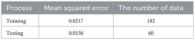
Table 10. Iteration summary for training and testing processes.

FIGURE 7

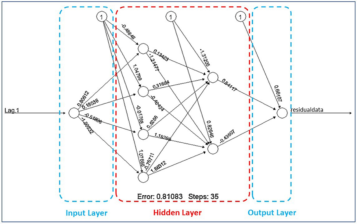
Figure 7. Architecture 1 − 4 − 2 − 1 of FFNN model with their weights for each unit.

For detail, the parameter estimation for each unit of the layers as the result of the iteration will be explained in two following Tables 11, 12.

TABLE 11

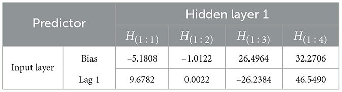
Table 11. Parameter estimation of FFNN model from input layer to hidden layer 1.

TABLE 12

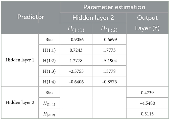
Table 12. Parameter estimation of FFNN model from hidden layer to output layer.

Based on Tables 11, 12, hidden layer 1 model of ARIMA(2,1,1) using FFNN(3,4,2,1) can be written to be:

$\begin{array}{c}{H}_{(1:1)}=f_p^{h1}(w_{10}^{h1}+{\displaystyle \sum _{i=1}^1}{x}_{ti}{w}_{1i}^{h1})=f_p^{h1}(-5.1808+9.6782x_{t1})\\ H_{(1:2)}=f_p^{h1}(w_{20}^{h1}+{\displaystyle \sum _{i=1}^1}{x}_{ti}{w}_{2i}^{h1})=f_p^{h1}(-1.0122+0.0022x_{t1})\\ H_{(1:3)}=f_p^{h1}(w_{30}^{h1}+{\displaystyle \sum _{i=1}^1}{x}_{ti}{w}_{3i}^{h1})=f_p^{h1}(26.4964-26.2384x_{t1})\\ H_{(1:4)}=f_p^{h1}(w_{40}^{h1}+{\displaystyle \sum _{i=1}^1}{x}_{ti}{w}_{4i}^{h1})=f_p^{h1}(32.2706+46.5490x_{t1})\end{array}$

and also the hidden layer 2 models of ARIMA(2,1,1) using FFNN(3,4,2,1) can be written to be:

$\begin{array}{l}{H}_{(2:1)}=f_p^{h2}(w_{10}^{h2}+{\displaystyle \sum _{i=1}^4{x}_{ti}}{w}_{1i}^{h2})\\ =f_p^{h2}(-0.9056+0.7243H_{(1:1)}+1.2778H_{(1:2)}\\ -2.5755H_{(1:3)}-0.6406H_{(1:4)})\\ =\frac{1}{1+e^{-0.9056+0.7243H_{(1:1)}+1.2778H_{(1:2)}-2.5755H_{(1:3)}-0.6406H_{(1:4)})}}\\ H_{(2:2)}=f_p^{h2}(w_{20}^{h2}+{\displaystyle \sum _{i=1}^4{x}_{ti}}{w}_{2i}^{h2})\\ =f_p^{h2}(-0.6699+1.7773H_{(1:1)}-5.1904H_{(1:2)}\\ +1.3778H_{(1:3)}-0.8576H_{(1:4)})\\ =\frac{1}{1+e^{-0.6699+1.7773H_{(1:1)}-5.1904H_{(1:2)}+1.3778H_{(1:3)}-0.8576H_{(1:4)})}}\end{array}$

By substituting the units of the hidden layer 1 and 2 into y_t1 as the output layer, the residual model of ARIMA(2,1,1) ε_t using FFNN(3,4,2,1) can be written as follows:

$\begin{array}{l}{ϵ}_t=y_{t1}=f_j^o(w_{10}^o+w_{11}^o{H}_{(1:1)}+w_{12}^o{H}_{(1:2)})\\ =\frac{1}{1+e^{-(0.4739-4.5480H_{(2:1)}+0.5115H_{(2:2)})}}& (37)\end{array}$

where x_t1, x_t2, x_t3 and y_t1 are normalized data from t-th actual data, that is the residual model of ARIMA(2,1,1).

3.4. The comparison between three models of exchange rate US dollar - ID rupiah

After getting the three estimated numerical models, such as ARIMA(2,1,1)-GARCH(1,1), ARIMA(2,1,1)-FFNN(3,4,2,1), and ARIMA(2,1,1)-GARCH(1,1)-FFNN(1,4,2,1), graphically, it can be analyzed to illustrate how the actual data associate to its fitted ARIMA(2,1,1) model and its three estimated model of ARIMA(2,1,1)-GARCH(1,1), ARIMA(2,1,1)-FFNN(3,4,2,1), and also ARIMA(2,1,1)-GARCH(1,1)-FFNN(1,4,2,1) in Figures 8A–C, respectively, as shown as in the following Figure 8.

FIGURE 8

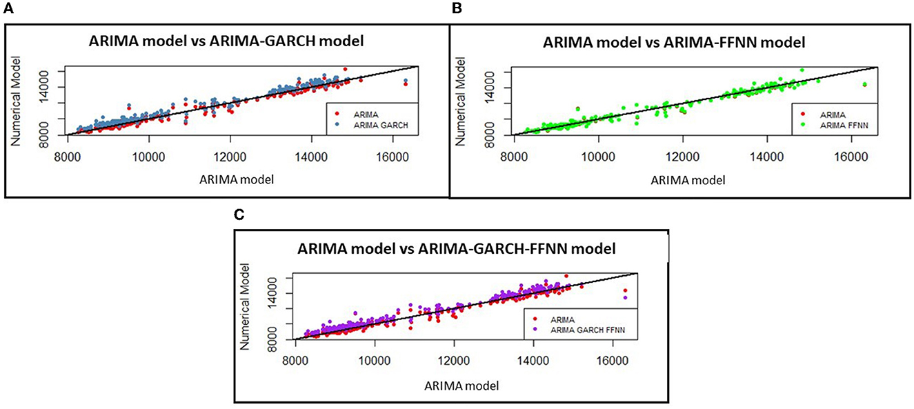
Figure 8. The comparison of actual currency exchange rate against its predicted values of ARIMA with (A) GARCH, (B) FFNN, and (C) GARCH-FFNN.

Figure 8 shows how the ARIMA(2,1,1) model in Figures 8A, C approaches the ARIMA(2,1,1) model. It can be described by the set of points between actual and fitted data forming a straight line y = x. The three ARIMA model data move closer to the straight line for improving the residual of the ARIMA model, which contains the heteroscedasticity effect. Therefore, it can be concluded that the fitted ARIMA(2,1,1) with three models has been good enough to model the exchange rate US dollar against the ID rupiah. Graphically, the result of the estimated values for ARIMA(1,1,1)-GARCH(1,1), of ARIMA(1,1,1)-FFNN(3,4,2,1), and of ARIMA(1,1,1)-GARCH(1,1)-FFNN(1,4,2,1) model will be shown respectively in Figure 9.

FIGURE 9

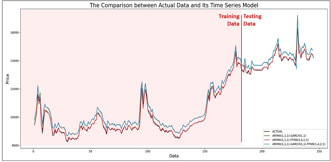
Figure 9. Comparison between data of actual currency exchange rate against predicted values of ARIMA with GARCH, FFNN, and GARCH-FFNN.

The result in Figure 9 shows that all ARIMA models with GARCH, FFNN, and GARCH-FFNN approach the actual value of currency exchange rate US dollar against ID rupiah. So that the results can reach good forecasting in application to real problems, and it will reduce the proportionality of the risks in running a business. To know what the best model is, the graphs in Figure 10 show the comparison of all ARIMA models graphically for 113th until 144th data.

FIGURE 10

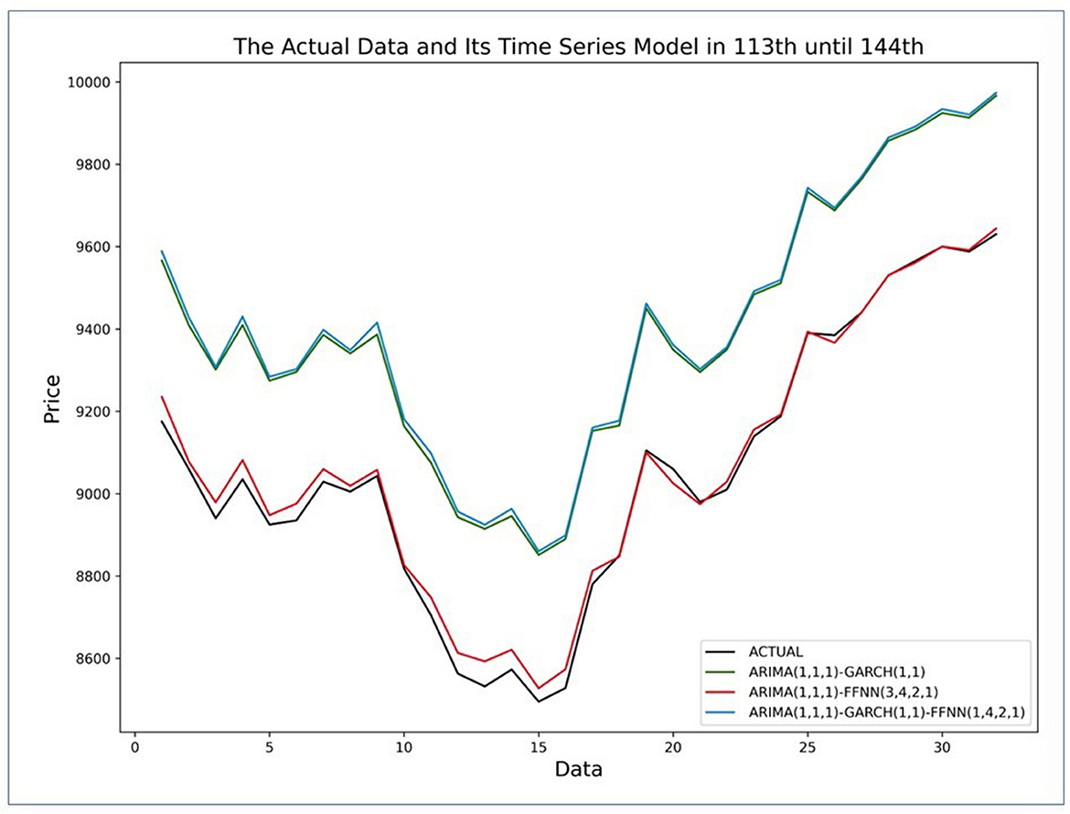
Figure 10. Comparison of 113th until 144th actual currency exchange rate against predicted values of ARIMA with GARCH, FFNN, and combination of GARCH and FFNN.

Based on Figure 10, there are four lines that are actual value (black) and three lines that are ARIMA model with GARCH (green), FFNN (red), and GARCH-FFNN (blue). The red line is more dominant in approaching the actual data than the green and blue lines. It shows that the ARIMA model with FFNN is better than other models. In contrast, the blue and green lines are almost close to the same value. It shows that the ARIMA with GARCH-FFNN is no significant difference from ARIMA with GARCH because the green line is always followed by the blue line. Besides, the argument based on Figure 10 is also evidenced by using measuring of forecast accuracy. Based on the result forecasting data for the currency exchange rate between the US dollar and ID rupiah, Table 13 shows the MSE and MAPE values.

TABLE 13

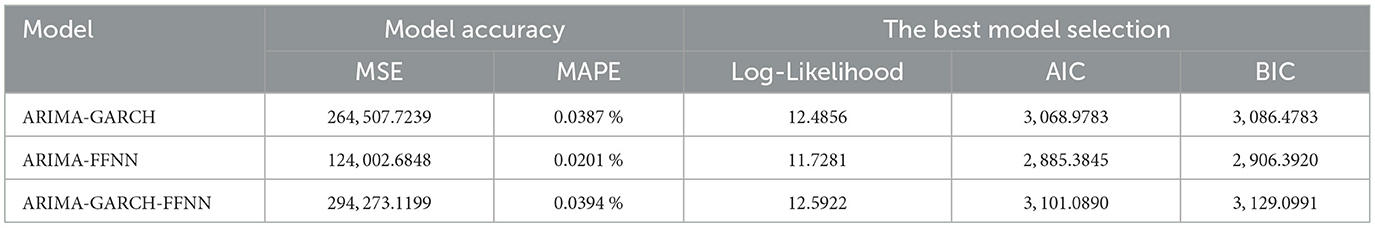
Table 13. Comparison of the ARIMA model with GARCH, FFNN, and GARCH–FFNN using model accuracy and the best model selection.

The result of Table 13 states that the model of ARIMA-FFNN has the smallest model accuracy of MSE and MAPE values. It shows that the model of ARIMA-FFNN is better used to forecast future value than the other two models. The ARIMA-FFNN obtains the currency exchange rate model using the numerical approach, and it is also the nonlinear model. As the numerical approach has a larger iteration, this method proposes the application of soft computing to obtain the estimation of the optimal weights precisely. Thus, the estimated parameters obtained by FFNN is getting better and approaching the actual value than linear model such as GARCH.

4. Discussion

In adjusting the heteroscedasticity on the time series model, some additional models linear or nonlinear are required. By using the case of the currency exchange rate, the heteroscedasticity effect that is included in the residual of the ARIMA(2,1,1) model can be adjusted by using the model of GARCH(1,1), the model of FFNN(3,4,2,1), or the hybrid model of GARCH(1,1)-FFNN(1,4,2,1).

These three additional models are then compared by calculating the model accuracy and the best model selection that is mentioned in Table 13. The result in Table 13 shows that the ARIMA-FFNN model is the best model for adjusting the heteroscedasticity. In addition, the prediction case of the exchange rate of the US Dollar against the Sri Lankan Rupee (USD/LKR) also showed that the ANN model performs better when compared with the GARCH model [17] and the techniques of SVR, GBM, and ARIMA to predict agricultural prices in Odisha, India [30]. For the other two models, the ARIMA-GARCH-FFNN has the MSE and MAPE value which is smaller than the ARIMA-GARCH, so the ARIMA-GARCH-FFNN is good enough to be used in modeling currency exchange rate US dollar - ID rupiah to solve heteroscedasticity problem such as the ARIMA-GARCH. These results are also reinforced by the previous research [31] where the hybrid algorithm has outperformed precision than the algorithm without hybridization. The comparison between the three additional models also shows that the ARIMA-GARCH-FFNN model, which is improving the ARIMA-GARCH model, is not always having better performance than the ARIMA-GARCH model. This result shows that there is a limitation of this study.

Overall, although the result shows that the ARIMA-FFNN be the best model for adjusting the heteroscedasticity effect, however, the presence of trend and time series data patterns have to be identified to know how the characteristics of these three additional model while adjusting the heteroscedasticity effect. By using the Diebold-Mariano Test, all models are checked to determine whether there is a significant difference between the two predicted models. Table 14 shows the result of the Diebold-Mariano Test for ARIMA-GARCH, ARIMA-FFNN, and ARIMA-GARCH-FFNN as follows:

TABLE 14

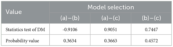
Table 14. The diebold-mariano test.

Based on Table 14, all probability values are greater than the significant level of 0.05. It means that there is no significant difference in solving the heteroscedasticity effect between the trend and time series data pattern of the two models of GARCH with FFNN, FFNN with hybrid GARCH-FFNN, and GARCH with hybrid GARCH-FFNN. In other words, the volatility effect that containing in the exchange rates data can be solved by using the model of ARIMA-GARCH, ARIMA-FFNN, and ARIMA-GARCH-FFNN. This statement is also stated by the previous research in estimating the Czech crown/Chinese yuan exchange rate where the additional parameters can help the equalized time series to retain order and precision [29]. Besides, the Diebold Mariano (DM) test was also applied to confirm the prediction accuracy of the wavelet-ANN model to forecast the occurrence of spiders in the pigeon pea [32].

5. Conclusion

In financial activities, the fluctuation of the financial data is a crucial problem in building a suitable time series. The classical time series model has usually analyzed its residual assumptions, such as autocorrelation, heteroscedasticity, and non-normality, to obtain the optimal fitted model. The heteroscedasticity effect often occurs in the model building because of the unstable fluctuations in the financial data. This study uses the financial data of currency exchange rate between US Dolar and ID Rupiah to build a suitable model of Autoregressive Integrated Moving Average (ARIMA). In adjusting the heteroscedasticity effect on the residual of ARIMA, this research uses three alternative methods, such as Generalized Autoregressive Conditional Heteroscedasticity (GARCH), Feed-Forward Neural Network (FFNN), and the combined model of GARCH-FFNN.

The three fitted performance models are observed monthly with 245 data using Mean Square Error (MSE) and Mean Absolute Percentage Error (MAPE). The results show that the accuracy model for the ARIMA(2,1,1)-GARCH(1,1), the model of ARIMA(2,1,1)-FFNN(3,4,2,1), and the model of ARIMA(2,1,1)-GARCH(1,1)-FFNN(1,4,2,1), respectively, are 99.9613%, 99.9799%, and 99.9606%. It shows that the ARIMA with FFNN has an accuracy value getting closer to 100%. It means that the ARIMA model with FFNN will be more approaching the actual value than the other two models because ARIMA-FFNN as the nonlinear model applies soft computing. The application of soft computing makes solving the numerical methodology easier in order to estimate the optimal fitted parameter precisely. Therefore, the estimated parameter of the FFNN method is more adjusting the heteroscedasticity effect than the classical method GARCH.

Data availability statement

Publicly available datasets were analyzed in this study. This data can be found at: https://www.bi.go.id/id/.

Author contributions

DD as the corresponding author conceptualized the study of the hybrid model to adjust the heteroscedasticity effect with the soft computing FFNN approach. MY organized the database and developed the simulation of the soft computing FFNN. MM performed the time series analysis of ARIMA–GARCH. FY analyzed the statistical method for obtaining the optimal parameter estimation of the model. All authors contributed to manuscript revision, read, and approved the submitted version.

Funding

The authors would like to acknowledge a research grant from the Indonesian Ministry of Education, Culture, Research, and Technology to support this excellence in basic research of the university project of the year 2021 with contract number 104/E4.1/AKA.04.PT/2021.

Conflict of interest

The authors declare that the research was conducted in the absence of any commercial or financial relationships that could be construed as a potential conflict of interest.

Publisher's note

All claims expressed in this article are solely those of the authors and do not necessarily represent those of their affiliated organizations, or those of the publisher, the editors and the reviewers. Any product that may be evaluated in this article, or claim that may be made by its manufacturer, is not guaranteed or endorsed by the publisher.

References

1. Riberio GT, Santos AAP, Mariani AC, Coelho LS. Novel hybrid model based on echo state neural network applied to the prediction of stock price return volatility. Expert Syst Appl. (2021) 184:115490. doi: 10.1016/j.eswa.2021.115490

CrossRef Full Text | Google Scholar

2. Pandey TN, Jagadev AK, Dehuri S, Cho SB. A novel committee machine and reviews of neural network and statistical models for currency exchange rate prediction: an experimental analysis. J King Saud Univ Comput Inf Sci. (2020) 32:987–99. doi: 10.1016/j.jksuci.2018.02.010

CrossRef Full Text | Google Scholar

3. Lu X, Que D, Cao G. Volatility forecast based on the hybrid artificial neural network and GARCH-type models. ScienceDirect. (2016) 91:1044–9. doi: 10.1016/j.procs.2016.07.145

CrossRef Full Text | Google Scholar

4. Paul RK. ARIMAX–GARCH–WAVELET model for forecasting volatile data. Model Assist Stat Appl. (2015) 10:243–52. doi: 10.3233/MAS-150328

CrossRef Full Text | Google Scholar

5. Gracia SJ, Rambaud SJ. A GARCH approach to model short-term interest rates: evidence from Spanish economy. Int J Financ Econ. (2020) 27:1621–32. doi: 10.1002/ijfe.2234

CrossRef Full Text | Google Scholar

6. Kambouroudis DS, McMillan DG, Tsakou K. Forecasting stock return volatility: a comparison of GARCH, implied volatility, and realized volatility models. J Futures Mark. (2016) 36:1127–63. doi: 10.1002/fut.21783

CrossRef Full Text | Google Scholar

7. Charles A, Darn é O. Volatility estimation for Bitcoin: replication and robustness. Int Econ. (2019) 157:23–32. doi: 10.1016/j.inteco.2018.06.004

CrossRef Full Text | Google Scholar

8. Lee J. A neural network method for nonlinear time series analysis. J Time Ser Econ. (2018) 11:1–18. doi: 10.1515/jtse-2016-0011

CrossRef Full Text | Google Scholar

9. Kumar G, Singh UP, Jain S. Hybrid evolutionary intelligent system and hybrid time series econometric model for stock price forecasting. Int J Intell Syst. (2021) 36:4902–35. doi: 10.1002/int.22495

CrossRef Full Text | Google Scholar

10. Zolfaghari M, Gholami S. A hybrid approach of adaptive wavelet transform, long short-term memory and ARIMA–GARCH family models for the stock index prediction. Expert Syst Appl. (2021) 182:115149. doi: 10.1016/j.eswa.2021.115149

CrossRef Full Text | Google Scholar

11. Babu CN, Reddy BE. A moving-average filter based hybrid ARIMA–ANN model for forecasting time series data. Appl Soft Comput. (2014) 23:27–38. doi: 10.1016/j.asoc.2014.05.028

CrossRef Full Text | Google Scholar

12. Zhang G, Hu MY. Neural network forecasting of the British Pound/US dollar exchange rate. Sci Direct. (1997) 26:495–506. doi: 10.1016/S0305-0483(98)00003-6

CrossRef Full Text | Google Scholar

13. Zhang GP. Time series forecasting using a hybrid ARIMA and neural network model. Sci Direct. (2003) 50:159–75. doi: 10.1016/S0925-2312(01)00702-0

CrossRef Full Text | Google Scholar

14. Henriquez J, Kristjanpoller W. A combined independent component analysis-neural network model for forecasting exchange rate variation. Appl Soft Comput. (2019) 83:105654. doi: 10.1016/j.asoc.2019.105654

CrossRef Full Text | Google Scholar

15. Vogt R, Touzel MP, Shlizerman E, Lajoie G. On lyapunov exponents for RNNs: understanding information propagation using dynamical systems tools. Front Appl Math Stat. (2022) 8:1–15. doi: 10.3389/fams.2022.818799

CrossRef Full Text | Google Scholar

16. Guresen E, Kayakutlu G, Daim TUN. Using artificial neural network models in stock market index prediction. Expert Syst Appl. (2011) 38:10389–97. doi: 10.1016/j.eswa.2011.02.068

CrossRef Full Text | Google Scholar

17. Nanayakkara S, Chandrasekara V, Jayasundara M. Forecasting exchange rates using time series and neural network approaches. Eur Int J Sci Technol. (2014) 3:65–73.

PubMed Abstract | Google Scholar

18. Adebiyi AA, Adewumi AO, Ayo CK. Comparison of ARIMA and artificial neural networks models for stock price prediction. J Appl Math. (2014) 2014:1–7. doi: 10.1155/2014/614342

CrossRef Full Text | Google Scholar

19. Devianto D, Maiyastri, Fadhilla DR. Time series modeling for risk of stock price with value at risk computation. J Appl Math Sci. (2015) 9:2779–87. doi: 10.12988/ams.2015.52144

CrossRef Full Text

20. Dritsaki C. The performance of hybrid ARIMA–GARCH modeling and forecasting oil price. Int J Energy Econ Policy. (2018) 8:14–21.

PubMed Abstract | Google Scholar

21. Yollanda M, Devianto D, Yozza H. Nonlinear modeling of IHSG with artificial intelligence. IEEE Explore. (2018) 83:85–90. doi: 10.1109/ICAITI.2018.8686702

CrossRef Full Text | Google Scholar

22. Devianto D, Permathasari P, Yollanda M, Ahmad AW. The model of artificial neural network and nonparametric MARS regression for Indonesian Composite Index. In: IOP Conference Series: Materials Science and Engineering. Bristol: IOP Publishing (2020). doi: 10.1088/1757-899X/846/1/012007

CrossRef Full Text | Google Scholar

23. Paul RK, Garai S. Performance comparison of wavelets-based machine learning technique for forecasting agricultural commodity prices. Soft Computing. (2021) 25:12857–73. doi: 10.1007/s00500-021-06087-4

CrossRef Full Text | Google Scholar

24. Berthiaume D, Paffenroth R, Guo L. Understanding deep learning: expected spanning dimension and controlling the flexibility of neural networks. Front Appl Math Stat. (2020) 6:1–17. doi: 10.3389/fams.2020.572539

CrossRef Full Text | Google Scholar

25. Russell SJ, Norvig P. Artificial Intelligence: A Modern Approach, Global Edition. Hoboken, NJ: Prentice Hall (2021).

PubMed Abstract | Google Scholar

26. Diebold FX, Mariano RS. Comparing predictive accuracy. J Bus Econ Stat. (1995) 13:253–63. doi: 10.1080/07350015.1995.10524599

CrossRef Full Text

27. Denis DJ. Applied Univariate, Bivariate, and Multivariate Statistics: Understanding Statistics for Social and Natural Scientists, with Applications in SPSS and R. Hoboken, NJ: Wiley. (2021). doi: 10.1002/9781119583004

CrossRef Full Text | Google Scholar

28. Mansour F, Yüksel MC, Akay MF. Predicting exchange rate by using time series multilayer perceptron. In: International Mediterranean Science and Engineering Congress, Vol. 3 (2019), p. 1–4.

PubMed Abstract | Google Scholar

29. Rowland Z, Lazaroiu G, Podhorska I. Use of neural networks to accommodate seasonal fluctuations when equalizing time series for the CZK/RMB exchange rate. Risks. (2021) 9:1–21. doi: 10.3390/risks9010001

CrossRef Full Text | Google Scholar

30. Paul RK, Yeasin M, Kumar P, Kumar P, Balasubramanian M, Roy HS, et al. Machine learning techniques for forecasting agricultural prices: a case of brinjal in Odisha, India. PLoS One. (2022) 17:1–17. doi: 10.1371/journal.pone.0270553

PubMed Abstract | CrossRef Full Text | Google Scholar

31. Paul RK, Garai S. Wavelets based artificial neural network technique for forecasting agricultural prices. J Indian Soc Probab Stat. (2022) 23:47–61. doi: 10.1007/s41096-022-00128-3

CrossRef Full Text | Google Scholar

32. Paul RK, Vennila S, Yeasin M, Yadav SK, Nisar S, Paul AK, et al. Wavelet decomposition and machine learning technique for predicting occurrence of spiders in pigeon pea. Agronomy. (2022) 12:1429 doi: 10.3390/agronomy12061429

CrossRef Full Text | Google Scholar