A maximum likelihood approach for asymmetric non-normal data using a transformational measurement model

Introduction

A popular method for parameter estimation in structural equation modeling (SEM) is the maximum likelihood estimation (MLE) method which was introduced in the late 1960's [1]. A major component of this estimation technique is the maximum likelihood function derived from the density function of a multivariate normal distribution. Recently, the long-standing popularity of this estimation method has been hampered, as the estimator has come under scrutiny because the validity of MLE outcomes is impaired when investigating non-normal data [2–4]. These outcomes suggest the restriction of MLE to investigations of data which closely follows a normal distribution.

Since much of the data investigated in applied situation are non-normally distributed, replacement and modification of MLE are options to explore. There are multiple ways to conduct alternative MLE including modified fitting functions [5, 6] and post-hoc corrections which take data characteristics into consideration (e.g., Satorra-Bentler method [7]). Furthermore, estimation methods based on a least-square approach are available [8, 9]. Recent studies compare two popular approaches: robust MLE with diagonally weighted least square estimation [10, 11]. These methods perform equally well in the presence of data commonly encountered by researchers such as: number of ordinal categories between four and ten, sample sizes between 200 and 1,000, and symmetric as well as asymmetric distributions. But, aside from the overall similarity in many situations, when MLE was applied to non-normal (asymmetrically distributed) data, parameter estimates by MLE yielded larger bias.

This essay reports on another possible modification of MLE for the purpose of improving its performance when analyzing data showing various degrees of non-normality. It takes the individual deviation of each observed variable into consideration and is not restricted to estimates of model fit. This modification is accomplished by a transformational measurement model that exerts influence on parameter estimation by use of the expectation-maximization (EM) algorithm [12, 13]. We characterize it as transformational because it is expected to shift the range of applicability from normally distributed data to asymmetric non-normal data.

In a way, the modification brought about by the transformational measurement model narrows the gap between MLE in factor analysis (including SEM) and outside of factor analysis where normality is rarely observed [14]. While in the context of factor analysis, MLE expects normally distributed data; however, in other applications MLE is recommended for dealing with non-normality [15]. An elaboration in line with this recommendation, for example, is an adaptation of MLE to the Rayleigh distribution [16].

For establishing the transformational measurement model as source of influence on EM algorithm, components of the model of the covariance matrix of MLE have to be related to corresponding components of the EM algorithm. This means re-parametrization of EM algorithm [17, 18]. In the course of re-parametrization it is necessary to assure that the performance of the algorithm is not impaired and that at the same time deviation from normality is taken into consideration.

Since non-normality as descriptive term applies to a variety of different distributions that may require different treatments, we restrict our research to a subset of non-normal distributions. The focus is on distributions that can be perceived as derived from a normal distribution by distortion (e.g., due to a scale restriction) in such a way that some properties are retained: the continuous scale, the existence of a major (i.e., global) peak as well as a mostly monotone increase up to this peak and a mostly monotone decrease following the peak. A major difference between original normal and non-normal data distributions is lack of symmetry. We characterize such distributions as asymmetric non-normal, abbreviated as asn (see Tables 1–3). The version of MLE described in this paper is optimized for investigating asn data.

TABLE 1

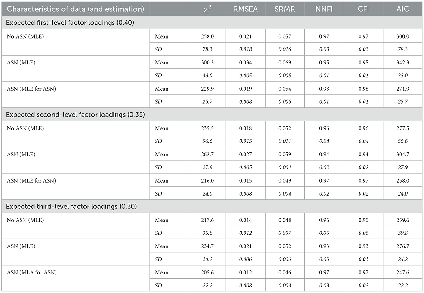
Table 1. Mean fit results and SDs (in italics) observed in investigating data showing (no) asymmetric non-normality (ASN) by one-factor models using regular MLE and MLE for ASN (N = 500).

The specification for asymmetric non-normal data is a characteristic that distinguishes the proposed version of MLE from other versions that are considered for non-normal data in general. Another characteristic is that parameters and fit statistics are estimated in the framework of a model reflecting the deviation of data from normality. This means that there is no post-hoc correction as found in other MLE versions. We refer to the proposed version of MLE as MLE for ASN.

The research reported in this paper was guided by two aims: (1) conceptualization of a version of MLE for asymmetric non-normal data within the framework of regular MLE for SEM by combining it with a transformational measurement model, and (2) demonstrating the efficiency of this version in investigating the structure of asymmetric non-normal data. MLE for ASN was also applied to asymmetric non-normal data with one-dimensional and two-dimensional underlying structures and compared with weighted least squares and diagonally weighted least squares methods.

The theoretical argument shows the following structure: at first, the model of the covariance matrix of MLE [19] is related to corresponding components of EM algorithm [13]. Subsequently, changes are introduced to fit the model to asymmetric non-normal data. Finally, the transformational measurement model is extracted.

The outset

We begin this investigation by considering the MLE fitting function, F, that is proposed for fitting the parameters of the theoretical model to data via the maximum likelihood criterion [1, 9, 15, 17]. This outset is selected since it provides information on what must be taken into consideration in order to demonstrate acceptable model-data fit. Let S (S ∈ ℜ^p×p) be the p × p empirical covariance matrix, Σ (Σ ∈ ℜ^p×p) the p × p model-implied covariance matrix that is specified by assigning value(s) to parameter(s), ϑ, and F() the MLE fitting function for model evaluation. MLE by definition refers to an iterative search for ϑ which provides the best fit of Σ to S on the basis of

$\begin{array}{cc}\text{F}\left[\Sigma (\vartheta ),\text{S}\right]& (1)\end{array}$

Whereas S is given and Σ reflects the assumptions of the tested model, ϑ is estimated while minimizing F in a succession of cycles of EM algorithm [12].

The model-implied covariance matrix, Σ(Σ ∈ ℜ^p×p), can show different degrees of complexity. For the purpose of the present study, we concentrate on the basic version with one latent variable for centered data associated with the congeneric measurement model [20] typically used with confirmatory factor analysis and structural equation modeling. This model includes two components that are expected to account for common and unique variation of data, respectively:

$\begin{array}{cc}\Sigma =\lambda \varphi {\lambda }^{\prime }+\Theta ,& (2)\end{array}$

with p × 1 vector λ (λ ∈ ℜ^p×1) of factor loadings on the latent variable of the corresponding measurement model, ξ [ξ ~ N(0, σ*)], variance parameter φ(φ ∈ ℜ⁺), and p × p diagonal matrix of residual variances Θ(Θ ∈ ℜ^p×p). Since λ and ϕ cannot be estimated at the same time, scaling is necessary [21]. This is frequently done by setting ϕ = 1.

Σ can also be viewed as a matrix composed of variances and covariances. Since variances are the more complex entries, which include two components, it is sufficient to concentrate the discussion on these components. The variance of ith manifest variable, σ_ii $({\sigma }_{ii}\in {\Re }^{+})$ (i = 1, …, p), is defined as

$\begin{array}{cc}{\sigma }_{ii}={\lambda }_i\varphi {\lambda }_i+{\theta }_i& (3)\end{array}$

where λ_i (λ_i ∈ ℜ) is the factor loading of the ith manifest variable on latent variable ξ, ϕ(φ ∈ ℜ⁺) the variance parameter and θ_i $({\theta }_i\in {\Re }^{+})$ the residual variance. In this model, ϕ measures the dispersion of the latent variable that is common to all manifest variables and, θ_i, the dispersion that is unique for the ith manifest variable.

In MLE the estimation of parameters is conducted by the EM algorithm. This method is a tool for the iterative estimation of parameters according to the maximum likelihood principle [22]. It is employed in situations such as missing information under the normal distribution assumption and mixture distributions [23]. The EM algorithm is considered important throughout statistics. Of importance for the present research is its application to factor analysis [13]. Employed as part of MLE, EM performs parameter estimation under the assumption of the normal distribution. Therefore, in the present study the consequences of deviations from normality reflected by the transformational measurement model for parameter estimation by EM algorithm need to be analyzed in some detail.

As the EM algorithm for factor analysis plays a major role in MLE for ASN, we proceed by recognizing the relationship between the parameters of Equation 3 and the parameters of EM algorithm. Furthermore, distributional assumptions need to be taken into consideration. EM-theory for factor analysis [13] assumes latent variables (i.e., factors) established by unobservable factor scores, which are symbolized as Z (Z ∈ ℜ^n×p). These factor scores are assumed to follow a normal distribution. This means that latent variables can be considered as normal through factor scores. EM theory also considers observed scores that are symbolized by Y (Y ∈ ℜ^n×q). In MLE they are also assumed to follow a normal distribution [1, 19].

Adaptation of the model described by Equation 3 to the notation of EM algorithm requires linking parameters λ, θ and ϕ of λ, ϕ and Θ to parameters of β, τ² and R [13] in corresponding order. Matrix β is defined as the “regression coefficient matrix” that “is commonly called factor-loading matrix” (p. 70), and matrix τ² as matrix “of residual variances … commonly called the uniquenesses” (p. 70). Furthermore, matrix R is defined as correlation matrix of the unobservable factor scores. We assume dimensionalities and data types for the EM matrices corresponding to the matrices of Equation 2. The symbol equivalent to ϕ is R^* since in a one-factor model R reduces to a 1 × 1 matrix, i.e., a scalar that is signified by the added star. It can be set free for estimation (see [13], Case 3). After a few EM cycles, this free parameter is likely to no more demonstrate the property of a (Pearson) correlation but may serve as estimate of common latent variation. Finally, σ_ii (Equation 3) is re-written using parameters of β, τ² and R as

$\begin{array}{cc}{\sigma }_{ii}={\beta }_{i}R*{\beta }_i+{\tau }_{ii}^2.& (4)\end{array}$

The preparation of EM algorithm for data non-normality

In this section, the model for normally distributed data is slightly modified to make it suitable for investigating asymmetric non-normal data while the basic definitions and assumptions of EM algorithm except of the ones regarding Y are retained.

The investigation of asymmetric non-normal data requires the establishment of a relationship between normally distributed data and asymmetric non-normal data. Recall at this point that asymmetric non-normal data are assumed to originate from normally distributed data by distortion (see Introductory section). We consider such a relationship at the level of variances (and covariances) since variances (and covariances) serve as input to SEM. We assume that the effect of distortion is reflected by distortion coefficient ${\alpha }_i^2$ $({\alpha }_i\in {\Re }^{+})$ (i = 1, …, p) linking the variance of the manifest variable representing asymmetric non-normal data [σ_ii(asn)] to the variance of the (corresponding) manifest variable representing normally distributed data [σ_ii(n)]:

$\begin{array}{cc}{\sigma }_{ii\text{(asn)}}={\alpha }_i^2{\sigma }_{ii(n)}.& (5)\end{array}$

In the following several transformations are described that are necessary for performing parameter estimation that is in line with Equation 5 by available SEM software including EM algorithm. In the first step, σ_ii(n) is replaced by its constituents (see Equation 3) so that its common and residual components can be treated separately. In the next step, the distortion coefficient is associated with each one of the two components so that

$\begin{array}{cc}{\sigma }_{ii\text{(asn)}}={\alpha }_i^2{({\lambda }_i\varphi {\lambda }_i)}_{ii(n)}+{\alpha }_i^2{\theta }_i.& (6)\end{array}$

In the following steps, ${\alpha }_i^2$ and θ_i are merged to give θ_i(asn) on one hand and on the other hand scalar ${\alpha }_i^2$ $({\alpha }_i\in {\Re }^{+})$ is subdivided and used for multiplying the common component included in parentheses from the left-hand side and the right-hand side. Since ϕ represents the dispersion of normally distributed latent variable ξ, this is signified by adding a subscript; it is written as ϕ_(n):

$\begin{array}{cc}{\sigma }_{ii(\text{asn})}={\alpha }_i({\lambda }_i{\varphi }_{(\text{n})}{\lambda }_i){\alpha }_i+{\theta }_{i(\text{asn})}.& (7)\end{array}$

Finally, we introduce an assumption that enables equal treatments of all manifest variables. It is assumed that the latent variable equally contributes to all manifest variables. This is a useful assumption for simulation studies and can also apply to empirical data under appropriate conditions. It allows setting λ_i = 1 (i = 1, …, p) so that the product of variance parameter and factor loadings, λ_i ϕ λ_i, can be replaced by ϕ_common(n) (= 1ϕ_(n)1) that is the same for all manifest variables (i = 1, …, p):

$\begin{array}{cc}{\sigma }_{ii(\text{asn})}={\alpha }_i{\varphi }_{\text{common}(\text{n})}{\alpha }_i+{\theta }_{i(\text{asn})}.& (8)\end{array}$

This expression includes a parameter that reflects normality of the latent variable, ϕ_common(n), and distinguishes parts that relate to asymmetric non-normality, α_i, or are influenced by it, θ_i(asn). It implies re-scaling: ϕ is set free while the replacement of the factor loading is fixed.

Following the final transformation we note the compatibility with EM algorithm. According to Case 3 of EM algorithm [13], β_i of β_i$R^{*}{\beta }_i$ (see Equation 4) can be fixed while R^* be free. Therefore, we set β_i equal to α_i (Equation 8) and R^* equal to ϕ_common(n) (Equation 8). Furthermore, since the description of EM algorithm does not includes a distributional assumption regarding τ², τ² is set equal to θ_i(asn). Writing Equation 8 accordingly gives

$\begin{array}{cc}{\sigma }_{ii(\text{asn})}={\beta }_{(\text{EM},\text{fixed})i}{R}_{(\text{EM},\text{estimated})}^{*}{\beta }_{(\text{EM},\text{fixed})i}+{\tau }_{(\text{EM},\text{estimated})i}^2& (9)\end{array}$

that is in line with Equation 4. Subscripts added; parentheses indicate a role in EM algorithm and whether the element is estimated or fixed.

Parameter estimation by EM algorithm occurs in cycles. Within each cycle R^* under the condition of Case 3 is estimated by means of a regression coefficient, δ, applied to the empirical covariance matrix. Here, δ is determined by β as well as the previous estimate of R^* [13]. Furthermore, residual matrix, Δ, with β and the previous estimate of R^* as components also exerts influence on revised R^* [13]. This means that the fixed β (i.e., α²) parameter upholds the relationship between what is expected to follow the normal distribution and what appears as distributional distortion.

Quantification of deviation from normality

This section presents a description of quantifying distortion coefficients, ${\alpha }_i^2$ (i = 1, …, p) (see Equation 5). Distortion coefficients are assumed to reflect the effect of distorting normally distributed data regarding their variances. Since σ_ii(n) and σ_ii(asn) of Equation 5 are unknown, ${\alpha }_i^2$ is not obtainable by rearranging the ingredients of Equation 5. Here, what is possible is using the possible proportionality of ${\alpha }_i^2$ (i = 1, …, p) and σ_ii(asn) (i = 1, …, p). For this purpose all αs and σ_(asn)s are arranged as p × 1 vectors. They show proportionality if σ_ii(n) (i = 1, …, p) can be assumed to be constant:

$\begin{array}{cc}\left[\begin{array}{c}{\alpha }_1^2\\ {\alpha }_2^2\\ {\alpha }_3^2\\ ⋮\\ {\alpha }_p^2\end{array}\right]\propto \left[\begin{array}{c}{\sigma }_{11\text{(asn)}}\\ {\sigma }_{22\text{(asn)}}\\ {\sigma }_{33\text{(asn)}}\\ ⋮\\ {\sigma }_{pp\text{(asn)}}\end{array}\right].& (10)\end{array}$

The equality assumption of factor loadings leading to Equation 8 justifies Equation 10.

Although σ_(asn)s are unknown, they demonstrate a property that can be employed for arriving at values that approximate αs. This property is that each σ_ii(asn) (i = 1, …, p) is expected to reflect the observed variance of corresponding asymmetric non-normal data, s_ii (i = 1, …, p) of S. This expectation implies that σ_ii(asn) shows a size similar to the size of s_ii:

$\begin{array}{cc}{\sigma }_{ii\text{(asn)}}\approx S_{ii}.& (11)\end{array}$

Together Equations 10 and 11 suggest a vector of variances obtained from distorted data for adjusting the statistical model to the effect of distortion. Furthermore, Equations 8 and 9 suggest the replacement of α²s by their square roots as well as ss by their square roots: let $\widehat{\alpha }$ $(\widehat{\alpha }\in {\Re }^{p\times 1})$ be the p × 1 vector of observation-based distortion coefficients corresponding to the standard deviations observed in distorted data. Then

$\begin{array}{cc}\widehat{\alpha }=\left[\begin{array}{c}{\widehat{\alpha }}_1\\ {\widehat{\alpha }}_2\\ {\widehat{\alpha }}_3\\ .\\ .\\ .\\ {\widehat{\alpha }}_p\end{array}\right]=\left[\begin{array}{c}{s}_1^{1/2}\\ s_2^{1/2}\\ s_3^{1/2}\\ \\ \\ \\ s_p^{1/2}\end{array}\right].& (12)\end{array}$

The hat (^∧) on top of α and αs is added to signify that observations serve as source.

The transformational measurement model for asymmetric non-normal data

Finally, the transformational measurement model is achieved by determining the measurement model associated with Equation 8 (i.e., finding the measurement model giving rise to Equation 8) with deviation coefficients according to Equation 12:

$\begin{array}{cc}\text{x}=\widehat{\alpha }\xi +\delta & (13)\end{array}$

including p × 1 vector x (x ∈ ℜ^p×1) of centered manifest variables, p × 1 vector $\widehat{\alpha }$$(\widehat{\alpha }\in {\Re }^{p\times 1})$ of distortion-reflecting fixations replacing fixed factor loadings (see Equation 12), latent variable ξ and p × 1 vector δ (δ ∈ ℜ^p×1)of residual variables. This model is proposed for investigating the hypothesis that the systematic variation of data is due to one underlying dimension (i.e., structural validity) if data show asymmetric non-normality.

Checking the compatibility with fitting function F

This section addresses the question whether fitting function F (Equation 1) is appropriate for asymmetric non-normal data. There is the original version of F derived from the density function of normally distributed data [1, 15]. Furthermore, there is an extended version that is implemented in current SEM software. It is an extended version that shows a special characteristic which broadens the field of application. It is defined as

$\begin{array}{cc}\text{F}=log\left|\Sigma \right|+\text{tr}(\text{S}{\Sigma }^{-1})-log\left|\text{S}\right|-p& (14)\end{array}$

where Σ (Σ ∈ ℜ^p×p) and S (S ∈ ℜ^p×p) represent the p × p model-implied and empirical covariance matrices in corresponding order and positive integer p the number of manifest variables [9, 17].

The special characteristic of this version is that in the case of a correct model (including correct parameter estimates), Σ_c, and data (an empirical covariance matrix) free of random influences, S_f: log|Σ_c| = log|S_f|, so that their difference is zero. Furthermore, in this case: S_f × Σ_c⁻¹ = I and tr(I) = p. Moreover, the difference of the trace of S_f × Σ _c⁻¹ and p is also zero so that,

$\begin{array}{cc}\text{F}\left[{\Sigma }_{\text{c}}\text{,}{\text{S}}_{\text{f}}\right]=log\left|{\Sigma }_{\text{c}}\right|+\text{tr}({\text{S}}_{\text{f}}{{\Sigma }_{\text{c}}}^{-1})-log\left|{\text{S}}_{\text{f}}\right|-p=0.& (15)\end{array}$

In sum, in the case a correct model and data with no error influence, F can be expected to arrive at a value of zero, and it is not necessary to make assumptions regarding the distribution of data (but, the matrices involved in the equation must allow for the computation of a determinant and inverse).

The presence of random influences may not invalidate the previous reasoning. In this case the model has to correctly account for the systematic variation of data so that only unsystematic variation due to random influences remains that is reflected by the outcome of F. If there is reason for assuming that deviations from expectations due to random influences follow normal distributions, the outcome can be considered as a χ² statistic, as is in investigating normally distributed data.

Although the fitting function, F, was developed for normally distributed data, its extended version appears to be applicable to a wider range of data types if the described characteristics hold. This means that there is the possibility that Σ accounts for systematic variation of S computed from asymmetric non-normal data because of the adjustment by $\widehat{\alpha }$. When there are also remainders due to random influences, the outcome of computing F may follow a χ² distribution.

It should be noted that the F-based χ² is currently only of importance as a component for the calculation of some fit indices. Furthermore, model fit may also be evaluated by fit indices that do not include χ² as a primary ingredient (e.g., SRMR).

An evaluation using simulated data

The major aim of the evaluation was to demonstrate that the described measurement model in combination with MLE will improve performance in investigating the latent structure of data in the presence of asymmetric non-normality. This premise gave rise to two hypotheses: first, we hypothesized that when analyzing data illustrating asymmetric non-normality MLE for ASN would lead to better overall model fit compared to regular MLE. This hypothesis is based on the expectation that only MLE for ASN, but not regular MLE, could account for all systematic variation in distorted data. Second, we hypothesized that MLE for ASN would not provide an advantage over regular MLE in accounting for systematic variation unrelated to asymmetric non-normality. This hypothesis aimed at systematic variation that was neither reached by an incorrect model nor related to distributional deviation. MLE for ASN was not expected to account for this kind of systematic variation. Another aim was the comparison of MLE for ASN with two established estimation methods suggested to account to non-normality: robust DWLS and WLS.

To evaluate our claims, we conducted a simulation study. Structured random data with and without skewness manipulation were investigated by a measurement model corresponding to the model for data generation, that is a model assuming equal contributions of a common source to all items. For this purpose we generated normally distributed random data showing an underlying structure and manipulated their distribution for obtaining asymmetric non-normal data. In most investigations the structure of data was unidimensional. In additional investigations with incorrect (and corresponding correct) models the underlying structure was two-dimensional.

Method

Data generation started with three sets of 500 × 20 matrices of continuous and normally distributed data [N(0,1)] using a generation method described by [24]. Either one or two unrelated underlying dimensions characterized the matrices. The expected factor loading of the first set was 0.40, in the second set 0.35 and in the third set 0.30. We refer to these as data with expected first-level factor loadings, expected second-level factor loadings and expected third-level factor loadings in corresponding order. The expected residuals were set to the difference between 1 and the common variation of items (the squares of the corresponding expected factor loadings). Data matrices with two underlying dimensions were realized as the combination of two subsets of columns. In this case, columns 1–10 of a matrix were associated with the first dimension and columns 11–20 with the second one.

When analyzing real data outside of the current research project, the typical observation was that the items' deviation from a symmetric distribution varied. We attempted to simulate this characteristic of real data by restricting deviation from symmetry to 10 of the 20 columns and generated different degrees of deviation. This transformation from symmetric to asymmetric was conducted according to the following formula: x_asn = (x × k)^1/2/k, where x > 0. That is, that the data of a column were multiplied by integer k in the first step. Then the square root was computed and the result divided by k. The integer, k, was set to 4 in transforming two columns of a matrix, to 16 in another two, to 64 in further two, and also to 256 and 1,024 in two plus two more columns such that the amount of non-normality varied across columns.

The measurement model for the statistical investigation included one latent variable with fixed factor loadings (see Equation 13) whereas the variance parameter of the corresponding model-implied covariance matrix was set free for estimation, as also were the parameters included in the main diagonal of Θ (see Equations 8, 9). The factor loadings were fixed according to Equation. 12.

Parameter estimation was conducted by means of the MLE option in LISREL [25] (regular MLE and MLE for ASN). In addition to MLE, DWLS and WLS were employed for parameter estimation. The LISREL version of DWLS additionally performed robust estimation according to a Satorra-Bentler post-hoc correction method.

Results

In the following the results of investigating model fit are reported for the different data conditions (data with no ASN and data with ASN) using regular MLE and MLE for ASN (first section), for correct and incorrect models (second section), and for different estimation methods (MLE for ASN, DWLS, and WLS) (third section).

Effects of MLE versions in normal and non-normal data (hypothesis 1)

Fit results for normally distributed and asymmetric non-normal data investigated by regular MLE and MLE for ASN are included in Table 1.

The three sections of this table comprise fit results observed when investigating data with an expected factor loading of 0.40 (expected first-level factor loadings), of 0.35 (expected second-level factor loadings) and of 0.30 (expected third-level factor loadings).

The first row of the upper section includes the mean χ², RMSEA, SRMR, NNFI, CFI, and AIC for the one-factor model with regular MLE applied to normally distributed data and the second row corresponding standard deviations (SD). Using commonly accepted guidelines (e.g., RMSEA ≤ 0.6, SRMR ≤ 0.8, NNFI ≥ 0.95, and CFI ≥ 0.95), all model fit indices indicated good model fit [26]. The third row provides the mean results observed in investigating asymmetric non-normal data also using regular MLE and the fourth row corresponding SDs. All statistics showed a numeric impairment in comparison to values presented in the first row; however, only NNFI and CFI values were down to the cutoff for good model fit. The mean results obtained by MLE for ASN applied to asymmetric non-normal data are included in the fifth row and the corresponding SDs in the sixth rows. All fit indices obtained by MLE for ASN indicated good model fit (i.e., were lower respectively larger than the corresponding cutoffs).

The fit results reported in the second and third sections (expected second-level and third-level factor loadings) of Table 1 showed similar patterns as in the first one although numerically slightly worse degrees of model fit were signified. In these sections, asymmetric non-normal data led to the switch from good to acceptable model fit according to NNFI and CFI when there was no MLE for ASN. In contrast, MLE for ASN yielded good model fit.

In sum, investigations by regular MLE revealed the expected decrease in model fit in the presence of asymmetric non-normality while adjustment to asymmetric non-normality resulted in the return to the original degree of model fit (confirmation of hypothesis 1).

Effects of MLE versions in unrelated systematic variation (hypothesis 2)

Fit results for correct and incorrect models used in investigating normally distributed and asymmetric non-normal data with regular MLE and MLE for ASN are reported in Table 2.

TABLE 2

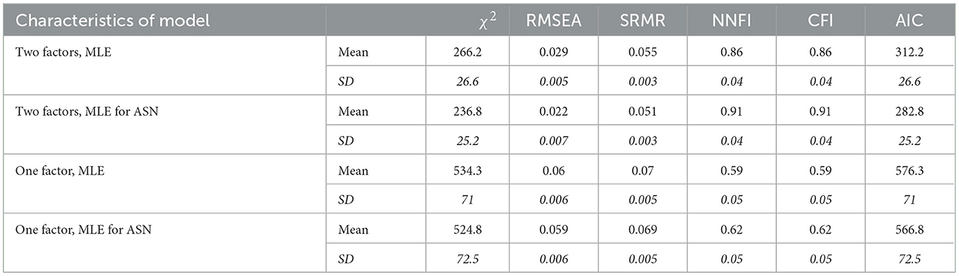
Table 2. Mean fit results and SDs (in italics) observed in investigating data showing (no) asymmetric non-normality (ASN) by one-factor and two-factor models using regular MLE and MLE for ASN (N = 500).

The first to fourth rows of this table include fit results for the correctly specified model and the remaining rows for the misspecified (i.e., incorrectly specified) model. The fit results for the correct model, but with no adaptation to asymmetric non-normality (first row), signified good model fit according to RMSEA and SRMR whereas NNFI and CFI illustrated model misfit. The report for the correct model with adaptation to asymmetric non-normality (third row) revealed improvement regarding NNFI and CFI to the level of acceptable model fit. All fit results for the incorrect models (see fifth to eights rows) were numerically worse than the fit results for the correct models (see first to fourth rows). The impairment in model fit was very obvious in NNFI and CFI results. These values were far below of what was considered as acceptable. Furthermore, in misspecified models, there was virtually no fit improvement due to adaptation to asymmetric non-normality, as was suggested by the second hypothesis.

In sum, MLE for ASN did improve model fit when the model was correct. In contrast, in incorrect models there was virtually no improvement (results in line with hypothesis 2).

Comparison of estimation methods

Finally, when analyzing asymmetric non-normal data, model fit was compared under MLE for ASN and alternative estimation methods, DWLS and WLS. In order to establish comparability, the alternative estimation methods were applied in combination with the one-factor model showing factor loadings fixed to the value of one, i.e., factor loadings reflecting the assumption of equal contributions of the latent source to all manifest variables.

Table 3 provides the mean fit results.

TABLE 3

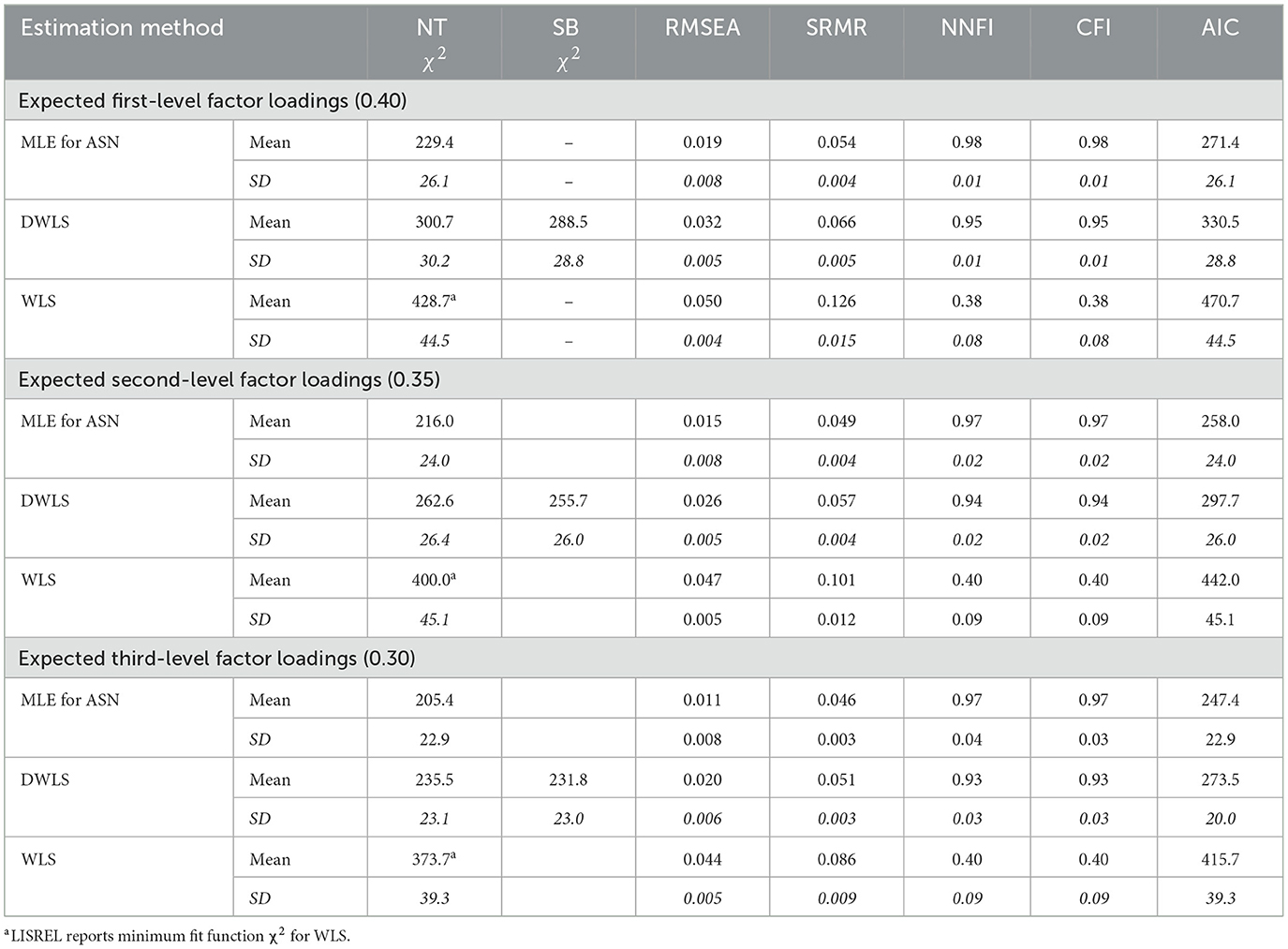
Table 3. Mean fit results and SDs (in italics) observed for MLE for ASN, DWLS and WLS in investigating data showing asymmetric non-normality (ASN) (N = 500).

Results presented in Table 3 follow the same structure as Table 1. There are three parts according to the expected factor loadings considered in data generation: expected factor loading of 0.40 (expected first-level factor loadings), of 0.35 (expected second-level factor loadings) and of 0.30 (expected third-level factor loadings). In each part the first and second rows repeat fit results of Table 1 for MLE for ASN, followed by DWLS and WLS results in corresponding order.

In each part, the fit results observed in investigating the data by MLE for ASN signified the numerically best model fit, DWLS the second best fit and the one obtained by WLS, ranked third. Furthermore, we investigated the difference between the statistics using the reported SDs. In data characterized by expected first-level factor loadings the difference between MLE for ASN and DWLS was larger than two SDs for χ², NNFI, CFI and AIC, and it was exactly two SDs for SRMR in data characterized by expected second-order factor loadings. WLS differed from MLE for ASN and from DWLS by more than two SDs in all comparison. Moreover, comparisons by CFI difference test [27] revealed substantial differences between all estimation methods for all data types.

Discussion

The maximum likelihood estimation method for factor analysis is closely linked to the concept of a multivariate normal distribution. The density function of a multivariate normal distribution provided the outset for creating the maximum likelihood fitting function [1], and unobservable data as the core component of parameter estimation by EM algorithm are assumed to follow a normal distribution [13]. Furthermore, normality of the remainders of fitting Σ to S is necessary to justify the assumption that the output of the maximum likelihood fitting function follows a χ² distribution [19]. Therefore, it is no surprise that analyzing non-normal data by regular MLE may not yield expected fit results.

Although the primary output of MLE, the χ² statistic, is currently rarely used in evaluating model fit, many alternative fit indices that are preferred instead [26] include the χ² statistic as ingredient in their calculations. The fit indices with cutoffs used in evaluating model fit show different degrees of sensitivity for deviation from a normal distribution in the reported study. NNFI and CFI showed considerable sensitivity for deviation whereas RMSEA and SRMR indicated good model fit under all conditions. The replacement of MLE by the other estimation methods revealed that SRMR was also to some degree sensitive to deviation from normality. Although RMSEA showed numeric impairment due to deviation from normality, there was no substantial difference according to the corresponding cutoff [27]. The mean RMSEA always signified good model fit, even in incorrect models.

The modification of MLE by using the transformational measurement model for the investigation of asymmetric non-normal data led to the expected improvement in model fit over regular MLE. When analyzing data in a variety of data types, the CFI difference [27] signified fit improvement. A substantial improvement was also observed by the RMSEA difference [27] in data with expected first-level factor loadings. Both MLE versions discriminated virtually equally well between correct and incorrect models. But there was no improvement due to MLE for ASN if systematic variation that was not otherwise reached was unrelated to distributional deviation.

To arrive at general statements regarding the performances of the estimation methods, we base the comparisons among these methods on the means reported in Tables 1–3 for one-factor models regarding the cutoffs for good model-data fit (RMSEA ≤ 0.6, SRMR ≤ 0.8, NNFI ≥ 0.95, and CFI ≥ 0.95). The percentages of reaching these cutoffs were 100 for MLE ASN, 66.6 for regular MLE, 66.6 for DWLS and 25 for WLS. The similar performances for regular MLE and DWLS are overall in line with results reported for these methods observed in investigating data showing less strong deviation from normality [10, 11]. The better performance of MLE for ASN is presumably restricted to data showing considerable deviation from normality. It is likely to do less well in overall normally distributed data.

An important but restricting assumption of MLE for ASN is the assumption of equal contributions of the latent source to all responses that justifies setting the factor loadings to equal sizes. The assumption of one latent variable as the source of responding is characteristic of customary confirmatory factor analysis [20] and the version of EM algorithm for confirmatory factor analysis [13]. But, in applied research, equal contributions of the latent source are rarely assumed so that factor loadings are mostly free for estimation. In investigating simulated data with expected factor loadings of the same size for all manifest variables, fixed factor loadings do not mean a disadvantage in comparison to free factor loadings [28]. Under appropriate conditions it may also apply for empirical data. Nevertheless, a version allowing for free factor loadings is desirable that, however, would require a more basic change of EM algorithm.

One limitation of the present study is the restriction to data distributions derived from a normal distribution by distortion. We concentrated on such asymmetric non-normal data because of our experiences with empirical research. The reason was that we observed that problems in reaching good model fit were frequently associated with data showing asymmetric non-normality. Another limitation is that distributions related to the normal distribution like beta, binomial and gamma distributions [29] are not taken into consideration. A further limitation is that we concentrated on model fit and omitted investigating bias in estimates. Future studies may include different simulation conditions to examine the viability of MLE for ASN under additional distribution and model conditions while including a variety of outcomes (e.g., parameter bias).

In summary, we present an alternative version of the maximum likelihood estimation (MLE) method for confirmatory factor analysis which includes a transformational measurement model. This transformational measurement model enables the investigation of the latent structure of asymmetric non-normal data. Furthermore, a simulation study is reported that demonstrates the efficiency of the method. An advantage in investigating asymmetric non-normal data over otherwise efficient robust DWLS and WLS is made apparent. We look forward to future research studies addressing these strengths and limitations of MLE for ASN.

Conclusion

The transformational measurement model opens up maximum likelihood estimation to data that deviate from a normal distribution that is otherwise a precondition for maximum likelihood estimation in factor analysis.

Data availability statement

The raw data supporting the conclusions of this article will be made available by the authors, without undue reservation.

Author contributions

KS conceptualized the study, performed the computations, and contributed to the writing. CD and BF shared ideas and contributed substantially to the writing. All authors contributed to the article and approved the submitted version.

Conflict of interest

The authors declare that the research was conducted in the absence of any commercial or financial relationships that could be construed as a potential conflict of interest.

Publisher's note

All claims expressed in this article are solely those of the authors and do not necessarily represent those of their affiliated organizations, or those of the publisher, the editors and the reviewers. Any product that may be evaluated in this article, or claim that may be made by its manufacturer, is not guaranteed or endorsed by the publisher.

References

1. Jöreskog KG. A general approach to confirmatory maximum likelihood factor analysis. Psychometrika. (1969) 34:183–202. doi: 10.1007/BF02289343

CrossRef Full Text | Google Scholar

2. Jobst LJ, Auerswald M, Moshagen M. The effect of latent and error non-normality on measures of fit in structural equation modeling. Educ Psychol Meas. (2021) 82:911–37. doi: 10.1177/00131644211046201

PubMed Abstract | CrossRef Full Text | Google Scholar

3. Lai K. Estimating standardized SEM parameters given non-normal data and incorrect model: methods and comparisons. Struct Equation Model. (2018) 25:1–21. doi: 10.1080/10705511.2017.1392248

CrossRef Full Text | Google Scholar

4. West SG, Finch JF, Curran PJ. Structural equation models with non-normal variables: problems and remedies. In: Hoyle R, , editor. Structural Equation Modeling: Concepts, Issues, and Applications. Thousand Oaks, CA: Sage (1995). p. 56–75.

Google Scholar

5. Yu C, Muthén B. Evaluation of model fit indices for latent variable models with categorical and continuous outcomes. In: Paper presented at the Annual Meeting of the American Educational Research Association (New Orleans) (2002).

PubMed Abstract | Google Scholar

6. Deng L, Yang M, Marcoulides KM. Structural equation modeling with many variables: a systematic review of issues and developments. Front Psychol. (2018) 9:1–14. doi: 10.3389/fpsyg.2018.00580

PubMed Abstract | CrossRef Full Text

7. Satorra A and Bentler PM. Corrections to test statistics and standard errors in covariance structure analysis. In: von Eye A, Clogg CC, , editors. Latent Variables Analysis: Applications for Developmental Research. Thousand Oaks: Sage (1994). p. 399–419.

Google Scholar

8. Arruda EH, Bentler PM, A. Regularized GLS for structural equation modeling. Struct Equation Model. (2017) 24:657–65. doi: 10.1080/10705511.2017.1318392

CrossRef Full Text | Google Scholar

9. Browne MW. Asymptotically distribution-free methods for the analysis of covariance structures. Br J Math Stat Psychol. (1984) 37:62–83. doi: 10.1111/j.2044-8317.1984.tb00789.x

PubMed Abstract | CrossRef Full Text | Google Scholar

10. Li CH. Confirmatory factor analysis with ordinal data: comparing robust maximum likelihood and diagonally weighted least squares. Behav Res Methods. (2016) 48:936–49. doi: 10.3758/s13428-015-0619-7

PubMed Abstract | CrossRef Full Text | Google Scholar

11. Li CH. Statistical estimation of structural equation models with a mixture of continuous and categorical observed variables. Behav Res Methods. (2021) 53:2191–213. doi: 10.3758/s13428-021-01547-z

PubMed Abstract | CrossRef Full Text | Google Scholar

12. Dempster AP, Laird NM, Rubin DB. Maximum Likelihood from Incomplete Data via the EM algorithm. J Roy Stat Soc B. (1977) 39:1–38. doi: 10.1111/j.2517-6161.1977.tb01600.x

CrossRef Full Text | Google Scholar

13. Rubin DB, Thayer DT. EM algorithms for ML factor analysis. Psychometrika. (1982) 47:69–76. doi: 10.1007/BF02293851

CrossRef Full Text | Google Scholar

14. Micceri T. The unicorn, the normal curve, and other improbable creatures. Psychol Bull. (1989) 105:156–66. doi: 10.1037/0033-2909.105.1.156

CrossRef Full Text | Google Scholar

15. Myung IJ. Tutorial on maximum likelihood estimation. J Math Psychol. (2003) 47:90–100. doi: 10.1016/S0022-2496(02)00028-7

CrossRef Full Text | Google Scholar

16. Lalitha S, Mishra A. Modified maximum likelihood estimation for Rayleigh distribution. Commun Stat A Theor. (2011) 25:389–401. doi: 10.1080/03610929608831702

PubMed Abstract | CrossRef Full Text | Google Scholar

17. Gelman A, Hill J. (2007). Data Analysis Using Regression and Multilevel/Hierarchical Models. New York, NY: Cambridge University Press (2007).

PubMed Abstract | Google Scholar

18. Hecht M, Gische C, Vogel D, Zitzmann S. Integrating out nuisance parameters for computationally more efficient Bayesian estimation—an illustration and tutorial. Struct Equation Model. (2020) 27:483–93. doi: 10.1080/10705511.2019.1647432

CrossRef Full Text | Google Scholar

19. Jöreskog KG. A general method for analysis of covariance structure. Biometrika. (1970) 57:239–57. doi: 10.2307/2334833

CrossRef Full Text | Google Scholar

20. Graham JM. Congeneric and (essentially) tau-equivalent estimates of score reliability. Educ Psychol Meas. (2006) 66:930–44. doi: 10.1177/0013164406288165

CrossRef Full Text | Google Scholar

21. Schweizer K, Troche S, DiStefano C. Scaling the variance of a latent variable while assuring constancy of the model. Front Psychol. (2019) 10:887. doi: 10.3389/fpsyg.2019.00887

PubMed Abstract | CrossRef Full Text | Google Scholar

22. McLachlan GJ. Computation: Expectation-Maximization Algorithm. International Encyclopedia of the Social and Behavioral Sciences (Second Edition). Amsterdam: Elsevier. (2016).

Google Scholar

23. Gumedze FN, Dunne TT. Parameter estimation and inference in the linear mixed model. Linear Algebra Appl. (2011) 435:1920–44. doi: 10.1016/j.Iaa.2011.04.015

PubMed Abstract | CrossRef Full Text | Google Scholar

24. Jöreskog KG, Sörbom D. Interactive LISREL: User's Guide. Lincolnwood, IL: Scientific Software International Inc. (2001).

25. Jöreskog KG, Sörbom D. LISREL 8.80. Lincolnwood, IL: Scientific Software International Inc (2006).

Google Scholar

26. DiStefano C. Examining fit with structural equation models. In: Schweizer K, Distefano C, , editors. Principles and Methods of Test Construction. Göttingen: Hogrefe Publishing (2016). p. 166–193.

Google Scholar

27. Cheung GW, Rensvold RB. Evaluating goodness-of-fit indexes for testing measurement invariance. Struct Equation Model. (2002) 9:233–55. doi: 10.1207/S15328007SEM0902_5

CrossRef Full Text | Google Scholar

28. Schweizer K, Ren X, Wang T, Zeller F. Does the constraint of factor loadings impair model fit and accuracy in parameter estimation? Int J Stat Prob. (2015) 4:40–50. doi: 10.5539/ijsp.v4n4p40

CrossRef Full Text | Google Scholar

29. Leemis LM, McQueston JT. Univariate distribution relationships. Am Stat. (2008) 62:45–53. doi: 10.1198/000313008X270448

CrossRef Full Text | Google Scholar