High-speed predictions of post-burn contraction using a neural network trained on 2D-finite element simulations

Introduction

Long-term contraction in burn injuries can lead to reduced joint mobilities. During this phenomenon, the wound reduces in size and deforms because of myofibroblasts (dermal cells) that contract. If the contraction of a scar leads to impairment of joint mobility, this is called scar contracture. Patient- and burn-specific factors influence contraction, such as the patient's age and gender, and the burn's size, depth, and location. These differences between burns and patients lead to the growing interest in personalized healthcare. Without medical care, a patient may have difficulty exercising or with simple daily activities, which we wish to prevent.

The theory of the physiological evolution of burned skin contains quantitative connections that are represented in mathematical relations. To give insight into significant elements influencing the contraction, we use detailed models such that we can tune these elements. We can use Monte Carlo simulations to assess the parameter's uncertainties, allowing for patient-specific predictions necessary for the clinic. However, high-dimensional mathematical models are expensive, a downside since many model-based predictions are needed to achieve personalized healthcare. Hence, we must use and develop alternatives to predict Monto Carlo-based post-burn contractions.

Neural networks can reflect complex relationships within a limited evaluation time after suitable training [1], which has been beneficial for years in the clinic. For example, Tran et al. have used computer vision to classify skin burns [2] and to classify tumors [3]. Furthermore, Brinati et al. have used neural networks to find diseases, such as the COVID-19 disease, in blood samples [4].

Our mathematical framework models deep skin burns in which the skin's dermis has burned. This framework focuses on post-burn contraction in this deep layer of the skin. The displacement of the dermis generates strains. Briefly, the model includes the structure of nine connected, non-linear partial differential equations. Four equations represent biochemical quantities, such as cell densities (two types), the concentration of signaling molecules, and collagen density. The other five equations track the entries of the strain matrix and the components of the velocity vector. The interaction between model variables reduces the wound/scar size, which we relate to the damaged tissue's relative surface area (RSA) density. Next to the RSA, we define the total strain energy (TSE) density, a measure of patient discomfort. In addition to our previous work in Egberts et al. [5], where we only predicted the evolution of the RSA, in this study, we train neural networks to predict the TSE and the wound/scar boundary. Others also used such surrogate models. For example, Cai et al. used three machine learning methods named K-nearest neighbor (KNN), XGBoost, and multi-layer perceptron (MLP) for parameter estimation of left ventricular myocardium [6]. The prediction of stress-strain curves for materials can be speeded-up by a convolutional neural network [7]. Further, neural networks can surpass other, non-intelligent acceleration techniques on both acceleration and accuracy [8]. In particular, Navratil et al. compare neural networks to other methods to accelerate the physics-based simulations in oil reservoir modeling and show a possible speedup of 2000X. In addition, neural networks reduces the average sequence error by two orders of magnitude.

This study explores using neural networks to replace the expensive finite-element predictions of post-burn contraction and patient discomfort. We apply the neural networks to the two-dimensional mathematical model because this two-dimensional model is expensive from a computational point of view. We construct a large dataset using our numerical approach by a Bayesian-like variation of parameter values. Then, we feed this dataset to feed-forward neural networks with two hidden layers. The resulting optimized networks are then implemented in an online application that illustrates possible future use.

In this article, Section 2 presents the mathematical model and its numerical implementation, and Section 3 presents the neural network. Subsequently, Section 4 presents the results and the illustrative (medical) application. Finally, Section 5 presents the conclusions, and Section 6 presents the discussion and further work.

The mathematical model

Our study uses the two-dimensional biomorphoelastic model for the post-burn contraction described in Koppenol et al. [9]. This model resembles post-burn contraction by dealing with chemical feedback that induces the skin's permanent displacement and the remaining effective Eulerian strain. The model takes the chemical feedback utilizing four chemical variables: the fibroblasts (N), the myofibroblasts (M), the signaling molecules (c), and collagen (ρ). Post-burn healing is initiated by releasing growth factors and cytokines (signaling molecules) that influence cell proliferation, myofibroblast differentiation, chemotaxis, and the synthesis and decay of collagen. For the cells, we consider migration toward the gradient of the signaling molecules [10] by a minimal model for chemotaxis [11], and cell density-dependent Fickian diffusion (random walk). The equations for the cell densities also contain a logistic-like cell proliferation term:

$\begin{array}{l}\frac{\text{D}N}{\text{D}t}+N(\nabla ·v)=-\nabla ·\left(-D_F(N+M)\nabla N+{\chi }_{F}N\nabla c\right)+\\ r_F\left[1+\frac{r_F^{\text{max}}c}{a_c^I+c}\right]\left[1-{\kappa }_F(N+M)\right]N^{1+q}-k_{F}cN-{\delta }_{N}N,& (1)\end{array}$

$\begin{array}{l}\frac{\text{D}M}{\text{D}t}+M(\nabla ·v)=-\nabla ·\left(-D_F(N+M)\nabla M+{\chi }_{F}M\nabla c\right)+\\ r_F\left[\frac{\left[1+r_F^{\text{max}}\right]c}{a_c^I+c}\right]\left[1-{\kappa }_F(N+M)\right]M^{1+q}+k_{F}cN-{\delta }_{M}M.& (2)\end{array}$

Here, D_F represents the (myo)fibroblast diffusion coefficient, and χ_F is the chemotactic parameter, r_F is the cell division rate, $r_F^{\mathrm{\text{max}}}$ is the maximum factor of cell division rate enhancement because of the presence of the signaling molecules, $a_c^I$ is the concentration of the signaling molecules that cause half-maximum enhancement of the cell division rate, κ_F(N + M) represents the reduction in the cell division rate because of crowding [12], q is a fixed exponent, k_F is the signaling molecule-dependent cell differentiation rate constant of fibroblasts into myofibroblasts, and δ_N, δ_M represent the apoptosis rates of the fibroblasts and myofibroblasts, respectively.

The signaling molecules only migrate because of (fickian) diffusion, and collagen is not subject to active migration. In both equations, (myo) fibroblasts are responsible for the secretion, and matrix metallo proteinases (MMPs) are responsible for the breakdown:

$\begin{array}{ll}\frac{\text{D}c}{\text{D}t}+c(\nabla ·v)=\nabla ·(D_c\nabla c)+k_c\left[\frac{c}{a_c^{II}+c}\right]\left[N+{\eta }^{I}M\right]-{\delta }_c\frac{\left[N+{\eta }^{II}M\right]\rho }{1+a_c^{III}c}c,& (3)\end{array}$

$\begin{array}{ll}\frac{\text{D}\rho }{\text{D}t}+\rho (\nabla ·v)=k_{\rho }\left[1+\left[\frac{k_{\rho }^{\text{max}}c}{a_c^{IV}+c}\right]\right]\left[N+{\eta }^{I}M\right]-{\delta }_{\rho }\frac{\left[N+{\eta }^{II}M\right]\rho }{1+a_c^{III}c}\rho .& (4)\end{array}$

Here D_c is the fickian diffusion coefficient of the signaling molecules, k_c is the maximum net secretion rate of the signaling molecules, η^I is the ratio of myofibroblasts to fibroblasts in the maximum secretion rate of the signaling molecules and collagen, $a_c^{II}$ is the concentration of the signaling molecules that causes the half-maximum net secretion rate of the signaling molecules, δ_c is the proteolytic breakdown rate parameter of the signaling molecules, η^II is the ratio of myofibroblasts to fibroblasts in the secretion rate of the MMPs and $1+a_c^{III}c$ represents the inhibition of the secretion of the MMPs. Further, k_ρ is the collagen secretion rate, $k_{\rho }^{\mathrm{\text{max}}}$ is the maximum factor of secretion rate enhancement because of the presence of the signaling molecules, $a_c^{IV}$ is the concentration of the signaling molecules that cause the half-maximum enhancement of the secretion rate of collagen and δ_ρ is the degradation rate of collagen.

Further, the model introduces the dermal displacement (u), the displacement velocity (v), and the infinitesimal effective strain tensor (ε). The equation for the displacement velocity is:

$\begin{array}{ll}{\rho }_t\left(\frac{\text{D}v}{\text{D}t}+v(\nabla ·v)\right)-\nabla ·\sigma =\text{f}=\nabla ·\left(\frac{\xi M\rho }{R^2+{\rho }^2}\text{I}\right),& (5)\end{array}$

where σ represents the dermal stress and f represents the cell traction-caused body force acting on the dermis. This equation represents the balance of momentum. Here ρ_t represents the total mass density of the dermal tissues, ξ is the generated stress per unit cell density and the inverse of the unit collagen concentration, and R is a body force-inhibiting constant. From a mechanical point of view, we assume the tissue to be isotropic and homogeneous, except for a dependency of the stiffness on the local collagen density [13]. The visco-elastic relation for the dermal stress is:

$\begin{array}{ll}\sigma ={\mu }_1\text{sym}(\nabla v)+{\mu }_2(\text{tr}(\text{sym}(\nabla v))\text{I})+\frac{E\sqrt{\rho }}{1+\nu }\left[\epsilon +\text{tr}(\epsilon )\frac{\nu }{1-2\nu }\text{I}\right],& (6)\end{array}$

where μ₁, μ₂ are the shear and bulk viscosity, respectively, $E\sqrt{\rho }$ represents Young's modulus (stiffness), and ν is the Poisson's ratio.

Finally, the equation for the effective Eulerian strain is:

$\begin{array}{ll}\frac{{D}\epsilon }{{D}t}+(\text{tr}(\epsilon )-1)\text{sym}(\nabla \text{v})=-\text{G}=-\zeta \frac{\left[N+{\eta }^{II}M\right]c}{1+a_c^{III}c}\epsilon ,& (7)\end{array}$

where $\frac{{D}\epsilon }{{D}t}=\frac{\text{D}\epsilon }{\text{D}t}+\epsilon \mathrm{\text{skw}}(\text{L})-\mathrm{\text{skw}}(\text{L})\epsilon$ is the Jaumann time derivative, and G is a growth contribution tensor. In the case of burns, it considers permanent deformation (in this case contraction) and permanent strains as a result of the changes in the chemical constitution of collagen. In the case of tissue of tumor development, it considers the actual growth. The parameter ζ is the rate of morphoelastic change.

Considering the boundary conditions, let ∂Ω_x the boundary of the computational domain. Then, for all time t and for all x ∈ ∂ Ω_x:

$\begin{array}{ll}N(\text{x},t)=N_{\text{eq}},M(\text{x},t)=M_{\text{eq}},c(\text{x},t)=c_{\text{eq}},\text{and}v(\text{x},t)=0.& (8)\end{array}$

It is unnecessary to specify any boundary conditions for ρ and ε because of overdetermination since we use v(x, t) = 0 on the boundary.

We solve the mathematical model utilizing the finite element method with linear basis functions. We apply the backward Euler method for time integration. We account for non-linearity by using inner Picard iterations. Further initial conditions and numerical methods are not essential for this work and are explained in detail in our earlier study [5].

Relative surface area and total strain energy

During wound healing, fibroblasts differentiate into myofibroblasts that exhibit contractile properties. Myofibroblasts express α-SM actin in microfilament bundles or stress fibers [14] that interact with the cell's surrounding tissue. If myofibroblasts disappear because of cell death, this contractile mechanism dies with the cell, and hence, the scar is not subject to this active myofibroblast contraction anymore. In the mathematical model, the scar remodels to equilibrium once the applied stress (active contraction) is released, and during this remodeling, the scar retracts. Therefore, the injured tissue's relative surface area (RSA) changes. One typical feature is the RSA density is its minimum value that corresponds with the maximum contraction during healing. After this moment, the RSA density converges to an asymptotic value, another typical feature of the RSA, as the scar remodels. The asymptotic RSA value shows the intensity of contraction after scar remodeling that might show a possible contracture.

The RSA density was compared to the average of clinical measurements of the RSA of placed unmeshed skin grafts after both early and late excision of burned skin data from Hadidy et al. [15] in Koppenol et al. [9]. For particular combinations of values for ζ and $a_c^{III}$ that directly relate to the tensor G (Equation 9), a good fit between the numerical method and the clinical data was obtained. We would like to train the neural network on clinical (non-synthetic) data, however, these data have privacy issues and it is not easy to find enough of that data.

Contracting wounds and scars lead to stress and strain on the skin, which can hypothetically lead to irritation (pain) and tingling sensations. The stress we refer to is the total strain energy we assume to measure patient discomfort. The total strain energy (TSE) is defined by the integral over the strain energy density (per unit volume) [16]. A typical feature of the TSE density is its maximum, i.e., the maximum post-burn discomfort that a patient might experience.

A neural network for post-burn scar contraction

The morphoelastic model for post-burn contraction has many patients- and wound-specific parameters for which we want to evaluate the uncertainty. However, considering this uncertainty using numerical simulations is costly because the model is highly non-linear. Therefore, we train neural networks to replace these (slow) simulations introduced in this section as an alternative.

Formulation

In our simulations, we use the computational domain ${\Omega }_{\text{x}}={(-10,10)}^2$ cm² where the subset $\left|\frac{x}{4}\right|+\left|\frac{y}{4}\right|\le 1$ (a rotated square) defines the initial wounded area. To reduce computation times, we perform computations on a quarter of this domain using symmetry. For the boundary conditions on the symmetry axes, let ${\Gamma }_{\text{x}}^s=\left\{(x,y):x=0,0\le y\le 10\right\}\bigcup \left\{(x,y):y=0,0\le x\le 10\right\}$. Then, for all $\text{x}\in {\Gamma }_{\text{x}}^s$, we have J_N/M/c·n = 0, v·n = 0 and (σ·n)·τ = 0, where n is the outward pointing normal vector and τ is the tangential vector. For the discretization of the domain, we use an adapted version of the KOKO mesh generator [17] to have a fine tuning of the mesh around the boundary of the wound (see Figure 1). For more information about our meshing strategy, we refer to our earlier study [5].

FIGURE 1

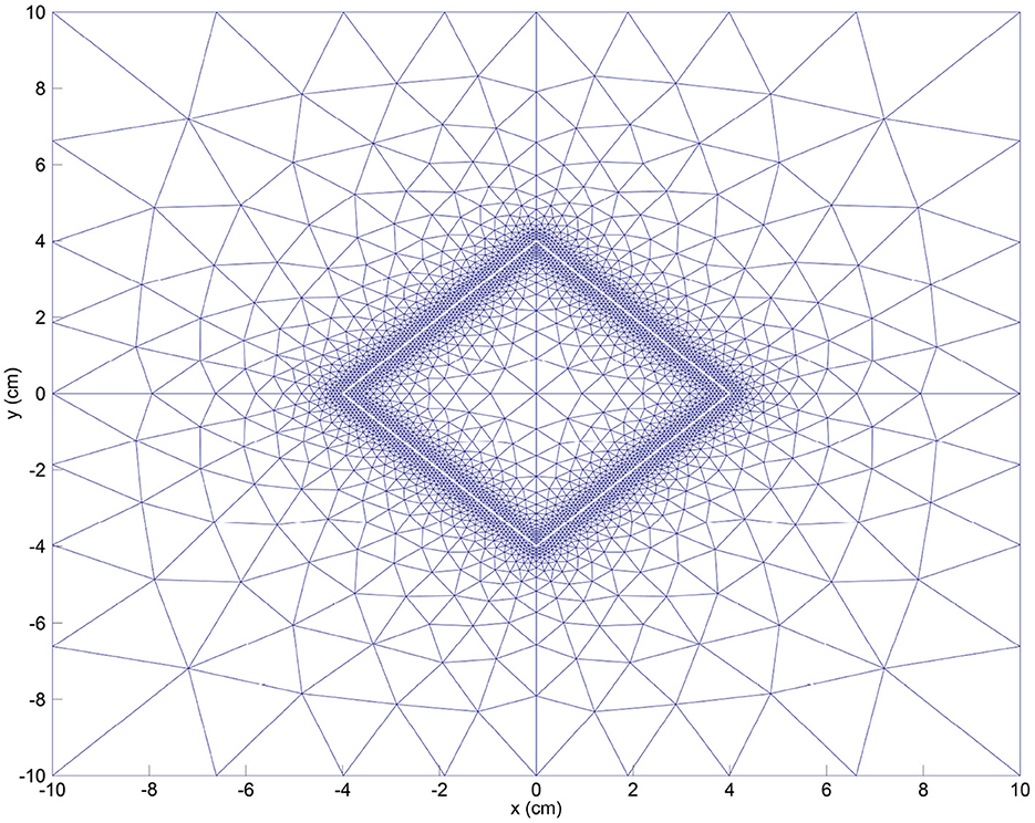
Figure 1. Initial mesh for the FEM (finite element method) discretization. We also show the initial wound boundary (in white).

The 25 independent parameter values make up the length of the input vector x that result in output variables y. Here, y ≈ f(x; θ) is either the non-dimensional RSA, the non-dimensional TSE, or the shape of the wound/scar boundary, determined by the numerical finite element-based model that simulates for 365 days using an adaptive time step. The data are post-processed to contain daily predictions and normalized between 0 and 1. The objective is to learn f(x; θ) ≈ y, with θ the learnable parameters of the feedforward networks. Our networks have two hidden layers, each with 100 neurons, and the rectified linear unit [18]. We use the sigmoid function on the output layer because the data bounds between 0 and 1. Remark that the RSA and TSE have 25 input and 365 output neurons. The number of output neurons for the wound/scar boundary is 42 × 365 because 21 points are used to describe the boundary.

Training, validating and testing

During the training of the neural networks, we use the Adamax algorithm with the standard backpropagation algorithm to minimize the mean squared error (MSE) loss [19]. The choice for Adamax follows from the learning rate range tests that we performed to determine the greatest learning rate value such that the networks are trained without discrepancy. For these tests, we vary learning rates between 0.0001 and 1 and then run for 150 epochs in batches of 64 samples. On average, the tests take around 7.2 min on a 64-bit Windows 10 Pro system with 16 GB RAM and a 3.59 GHz AMD Rizen 5 3600 6-Core Processor. Given the results, we choose initial learning rates of 0.015 for the RSA and the wound/scar boundary, respectively, and 0.004 for the TSE, with a standard decaying factor of 0.99. We stop training if the validation MSE loss shows no improvement in 50 epochs. We use the early stopping regularization to avoid model overfitting.

Data

The input dataset we use to train and test the neural networks has size n × 25 × 365 consisting of n = 5, 000 numerical simulations. We set acceptable values for each input parameter that varies between simulations and patients; therefore, the dataset is well-varied. We draw parameter samples from uniform statistical distributions based on the ranges. The model's stability condition [20] $k_c<{\delta }_c\overline{\rho }{a}_c^{II}$ defines acceptable samples. We use a domain of 10 cm² with a uniform triangulation with 968 nodes. Using Min-Max scaling, we split the dataset in train- and test sets, with an 80/20% train-test split.

Performance measures

We include the goodness-of-fit (R²) statistic that we maximize to minimize the L² norm (square error loss), the average relative root mean squared error (aRRMSE), and the average relative error (aRelErr).

Results

The neural networks predict the RSA, the TSE, and the wound/scar boundary. Figure 2 shows the best and the worst predictions for the MSE, the worst prediction relative errors, and the relationship between the predicted and target values in the RSA test set. Figure 2A shows the optimal prediction, where the RSA prediction mostly overlaps the RSA target for the first 130 days and underestimates slightly during the wound healing remodeling phase. In the worst-case scenario, shown in Figure 2B, the neural network shows a delay during contraction and retraction and overestimation during remodeling. The minimum shifted to day 58, compared to day 52 in the RSA target. During remodeling, the overestimation is about 1% less contraction. The worst prediction relative error increases to 9.4% and converges to about 1.39% for the last predicted value, as shown in Figure 2C. The error peaks around day 30, during steep contraction, while the relative error around the moment of maximum contraction is < 1%. Finally, Figure 2D shows the (target, prediction) distribution follows the y = x line. Outliers are because of the worst prediction. The spread in the range 0.75 ≤ x ≤ 0.95 shows that the neural network could have trouble predicting contraction values between these values.

FIGURE 2

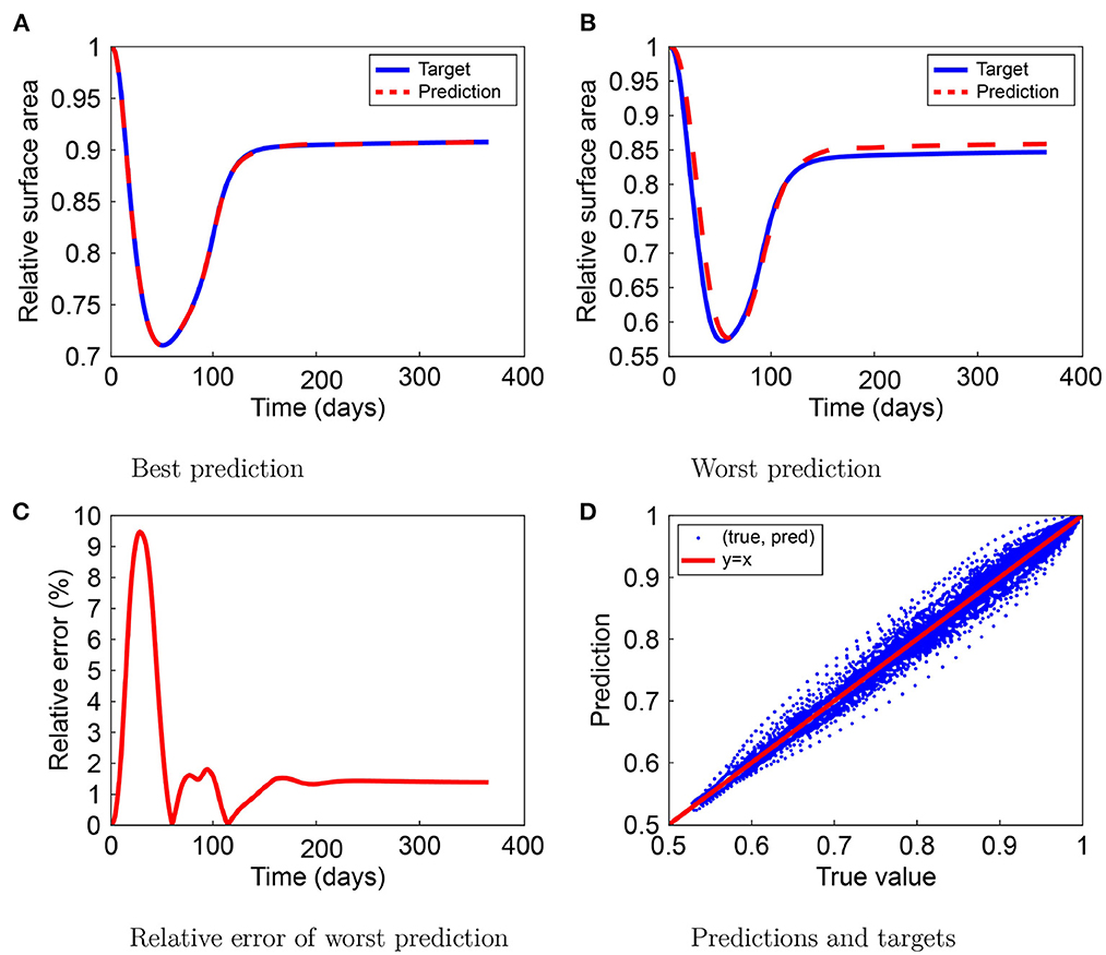
Figure 2. Results for the relative surface area (RSA) prediction by the neural network. The figure shows the best (A) and worst (B) predictions, the worst prediction relative error (C), and the prediction-target relation (D).

Figure 3 shows the best and the worst predictions for MSE, the worst prediction relative error, and the relationship between the predicted and target values in the TSE test set. In the best-case scenario, the TSE prediction mostly overlaps the TSE target, except for the maximum TSE around day 50, as Figure 3A shows a slight overestimation. In the worst-case scenario, shown in Figure 3B, the prediction by the neural network is almost indistinguishable from the TSE target value. Figure 3C shows the relative error of the worst TSE prediction and shows a maximum increase to 0.53% on day 23, which is negligible. Finally, Figure 2D shows that the (target and prediction) distribution follows the y = x line. The spread in the lower range shows that the neural network could have trouble predicting small TSE values and that larger values occur sporadically.

FIGURE 3

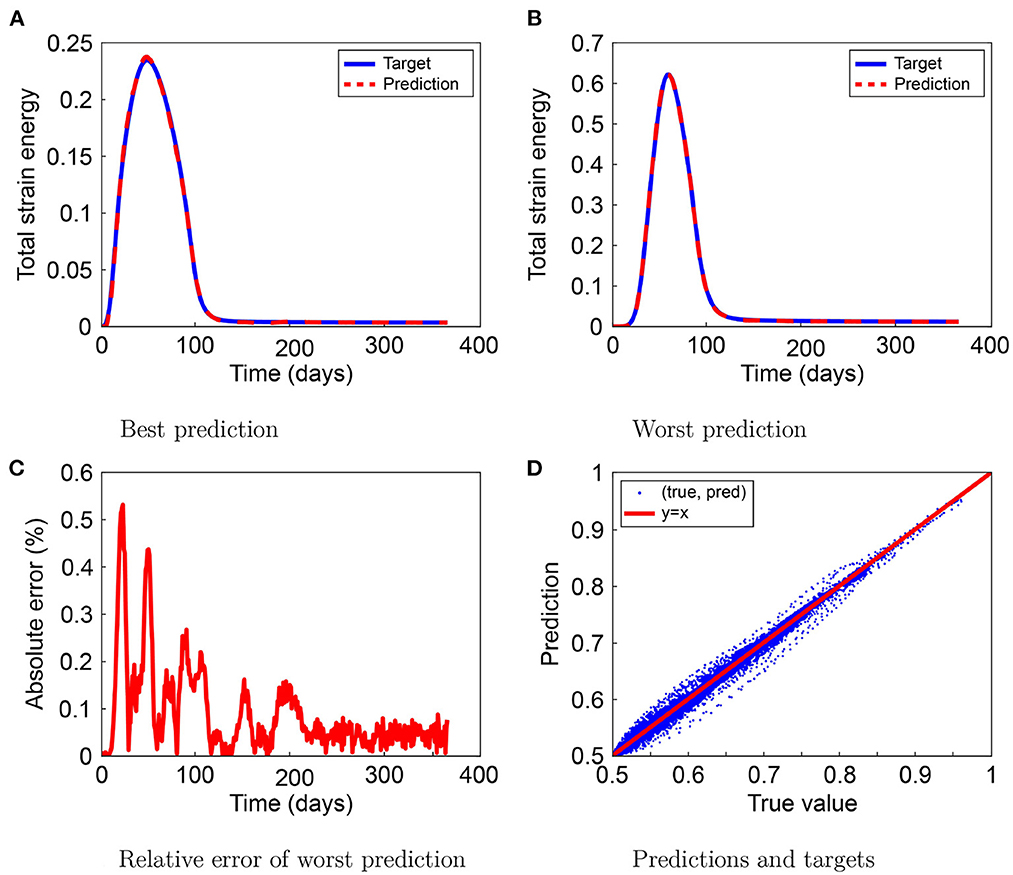
Figure 3. Results for the total strain energy (TSE) prediction by the neural network. The figure shows the best (A) and worst (B) predictions, the worst prediction relative error (C), and the prediction-target relation (D).

The RSA only provides information about the general contraction and lacks any information about localized contractions. Using the displacement of the wound/scar edge, we can also visualize the contraction and retraction of the wound/scar. Visualizing this movement is intuitively more straightforward to interpret than numeric values. Figure 4 shows the results of the neural network we trained to predict the wound/scar boundary. Here, we display targets and predictions on days 5, 25, 50, 75, and 365, with the targets in blue and the predictions in red. The days are shown in the average relative error for the best and worst predictions. We can see that in the case of the best prediction (upper graphs), the prediction follows the target closely. For the worst prediction (lower graphs), the prediction shows a slight deviation from the target boundary (less contraction) in the early phase of contraction, before maximum contraction has not been reached yet (day 25). Here, the predicted wound boundary is larger than the target boundary, which is also in line with the trend in Figure 2B. Further, the graphs show that the neural network can closely predict the wound/scar boundary.

FIGURE 4

Figure 4. Results from the neural network for the wound/scar edge. The upper graphs show the best predictions, while the lower graphs show the worst ones. In each graph, the blue line shows the target, and the red dashed line shows the neural network prediction.

In Table 1, we show the performances of the neural networks. We see that we obtained R² ≥ 0.9969 for all networks, which fits within the 95% interval of confidence. The aRRMSEs are 0.0787, 0.0864, and 0.0825 for the RSA, the TSE, and the wound/scar boundary, respectively, showing excellent performance according to Despotovic et al. [21]. The aRelErrs are only 0.018, 1.4919, and 0.0020%, confirming that the neural networks can predict the RSA, the TSE, and the wound/scar boundary. Subsequently, the networks predict 1,000 samples in only 0.2744 s (i.e., 0.2744 ms/sample). In contrast, the numerical simulations take, on average, 498 s per sample. Hence, we obtain a speedup of 1815000X, showing a remarkable acceleration. Taken together, these results confirm our observations.

TABLE 1

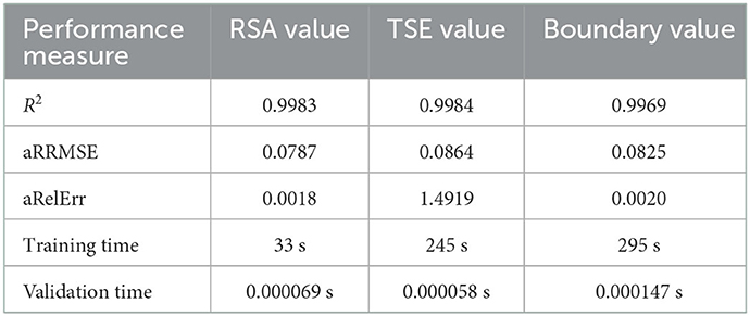
Table 1. Performance of the neural networks.

Focusing on specific characteristics during post-burn healing makes interpreting the neural network performances easier and is interesting in the clinic. These characteristics are the minimum and the asymptotic RSA values and the maximum TSE value, for which the performances are shown in Table 2. The R² of the minimum and asymptotic RSA values and the maximum TSE value are 0.9989, 0.9965, and 0.9990, respectively. Compared to the overall performance scores, the score for the asymptotic RSA is lower, though still above 99%, and the scores for minimum RSA and the maximum TSE are higher than the overall performance scores. The mean average errors (MAEs) are 0.0016 for the minimum RSA, 0.0009 for the asymptotic RSA, and 0.0029 for the maximum TSE, which are within 1% of the ranges (fifth column) of the minimum and maximum values. Further, these MAEs are within 1% of the average values (sixth column). These results support the networks' performances. The networks can recognize the minimum RSA within 51–83% and the asymptotic RSA within 81 and 95%. We note that the most significant absolute error of the asymptotic RSA value prediction is < 1.17%. In conclusion, our neural networks can predict these characteristics at different stages during healing and in ranges of parameter values.

TABLE 2

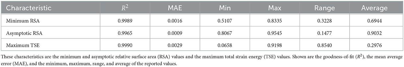
Table 2. Performances of the neural networks for specific characteristics during post-burn healing.

Application of the neural network

We prefer using a neural network instead of the numerical finite element method to quickly access the Monte Carlo simulations. We created a computational application to show the potential of the networks trained in this study. The app shows the effects of the uncertainties for the RSA, the TSE, and the wound/scar boundary and offers probabilities of contractures. To find age-related parameter values, we use interpolation in literature data based on our earlier study [5]. In short, the application reads the patient's age and then decides the parameter distributions. For illustration, the app shows other patient and wound-specific options that the app does not consider yet. The application that considers the burn of the rotated square, post-processes the Monte Carlo simulations and visualizes the results. After publication, the app can be downloaded from 4TU.Centre for Research Data.

Conclusions

The numerical approaches to post-burn contraction are less suitable for applications that require numerous simulations in a clinical environment since they are computationally expensive. Therefore, we study neural networks that serve as a low-cost alternative modeling strategy. After training, these neural networks provide compelling predictions for a post-burn scar. Our networks give aRellErr = 0.0018, 1.4919, and 0.0020% and R² = 0.9983, 0.9984, and 0.9969 for the RSA, the TSE, and the wound/scar boundary. Further, the networks accurately predict the minimum and asymptotic RSA values and the maximum TSE values. The minimum RSA reports MAE = 0.0016 and R² = 0.9989; for the final RSA, it reports MAE = 0.0009 and R² = 0.9965; and for the maximum TSSE, it reports MAE = 0.0029 and R² = 0.9990.

Furthermore, this machine learning approach gives a 1815000X speedup. This speedup allows for the Monte Carlo-based example application we developed and published. Our application considers the patient's age, demonstrating its effect on post-burn contraction and patient discomfort. Clinicians can tailor complication-dependent therapies if they can access such an application that predicts complications after a burn efficiently and reliably. Clinicians can then predict probabilities of success under various treatments and pathological circumstances. Given that the neural networks are effective and inexpensive, we can also use such an application for parameter studies and patient-oriented healthcare to optimize burn treatment.

Discussion and further work

Even though our neural networks can reproduce numerical data, there are plenty of discussion topics for numerical and machine learning models.

Our model is a minimalistic simplification of reality, which we want to keep the same since more complicated models are not necessarily better than so-called simple ones. The current model describes clinical observations smartly, though the model still needs to be completed. Let y_c represent clinical measurement, y denote the simulations by the finite element method, and f(x; θ) represent the predictions by the neural network model. Then, we realize that the total error between the neural network model and clinical observations is determined by

$\parallel y_c-f(x;\theta )\parallel =\parallel y_c-y+y-f(x;\theta )\parallel \le \parallel y_c-y\parallel +\parallel y-f(x;\theta )\parallel .$

Hence the overall error is bounded by the sum of the modeling error and the neural network error. In a future model, we want to implement the distinct collagen types and integrate the functioning of the immune system, which are significant factors influencing post-burn healing and scar formation. Besides the wound shape, three-dimensional models are capable of dealing with the depth of the wound. However, the numerical computational complexity is a drawback because of a decreasing mesh quality and the curse of dimensionality. These drawbacks can be solved by rotational symmetry and isogeometric analysis.

Because machine learning computations provide such a speedup, we expect this to be the way to integrate simulations into medical practice. Once we have further developed the numerical concepts, a practitioner can scan the burn, for example, using laser Doppler to map the blood flow in the wound. This scan contains the form (geometry) of the injury and its severity (in terms of blood flow). Such a scan can also include noise that we can filter using image processing, which may be kernel-based or machine-learning based.

Convolutional neural networks that work with images of the initial burn can fit the wound. For this, we need to extract contours and other features, which we can do with pixel-based statistics, shape similarity [22], and shape matching [23]. Further, the prediction of post-burn contraction is less complicated for standard geometries, such as squares and circles. We can use factors such as shape indices to integrate with these standard geometric objects. The edge error can measure such a mapping error [24]. In reality, burns do not heal at the same rates. Also, contractures can develop again after applied treatments dissolve these. In these instances, we need predictions over other periods. Hence, we need a network that can work with variable input and output, and therefore, we can use hybrid approaches (e.g., long-term memory). However, we still need a sizeable clinical dataset to train such a model.

Next to adapting the mathematical model and consider different neural network approaches, we plan to combine these finite element simulations with real patient-specific data to predict, to adapt and to improve therapies for burn injuries next to the common sense of clinicians. For this, we will collect clinical datasets from anonymized patients, including patient-observed data (POSAS).

Data availability statement

The datasets presented in this study can be found in online repositories. The names of the repository/repositories and accession number(s) can be found at: 4TU.ResearchData–DOI: 10.4121/21257199.

Author contributions

All authors listed have made a substantial, direct, and intellectual contribution to the work and approved it for publication.

Funding

This study was supported by Dutch Burns Foundation, Project 17.105.

Acknowledgments

The authors are grateful for the financial support by the Dutch Burns Foundation under Project 17.105.

Conflict of interest

The authors declare that the research was conducted in the absence of any commercial or financial relationships that could be construed as a potential conflict of interest.

Publisher's note

All claims expressed in this article are solely those of the authors and do not necessarily represent those of their affiliated organizations, or those of the publisher, the editors and the reviewers. Any product that may be evaluated in this article, or claim that may be made by its manufacturer, is not guaranteed or endorsed by the publisher.

References

1. Funahashi K. On the approximate realization of continuous mappings by neural networks. Neural Netw. (1989) 2:183–92. doi: 10.1016/0893-6080(89)90003-8

CrossRef Full Text | Google Scholar

2. Tran H, Le T, Nguyen T. The degree of skin burns images recognition using convolutional neural network. Indian J Sci Technol. (2016) 9:106772. doi: 10.17485/ijst/2016/v9i45/106772

CrossRef Full Text | Google Scholar

3. Mohsen H, El-Dahshan E, El-Horbaty E, Salem A. Classification using deep learning neural networks for brain tumors. Fut Comput Inform J. (2018) 3:68–71. doi: 10.1016/j.fcij.2017.12.001

CrossRef Full Text | Google Scholar

4. Brinati D, Campagner A, Ferrari D, Locatelli M, Banfi G, Cabitza F. Detection of COVID-19 infection from routine blood exams with machine learning: A feasibility study. J Med Syst. (2020) 44:4. doi: 10.1007/s10916-020-01597-4

PubMed Abstract | CrossRef Full Text

5. Egberts G, Desmoulière A, Vermolen F, van Zuijlen P. Sensitivity of a two-dimensional biomorphoelastic model for post-burn contraction. Biomech Model Mechanobiol. (2022) 22:1634. doi: 10.1007/s10237-022-01634-w

PubMed Abstract | CrossRef Full Text | Google Scholar

6. Cai L, Ren L, Wang Y, Xie W, Zhu G, Gao H. Surrogate models based on machine learning methods for parameter estimation of left ventricular myocardium. Royal Soc Open Sci. (2021) 8:201121. doi: 10.1098/rsos.201121

PubMed Abstract | CrossRef Full Text | Google Scholar

7. Yang C, Kim Y, Ryu S, Gu G. Prediction of composite microstructure stress-strain curves using convolutional neural networks. Mater Des. (2020) 189:108509. doi: 10.1016/j.matdes.2020.108509

CrossRef Full Text | Google Scholar

8. Navrátil J, King A, Rios J, Kollias G, Torrado R, Codas A. Accelerating physics-based simulations using end-to-end neural network proxies: An application in oil reservoir modeling. Front Big Data. (2019) 2:33. doi: 10.3389/fdata.2019.00033

PubMed Abstract | CrossRef Full Text | Google Scholar

9. Koppenol D, Vermolen F. Biomedical implications from a morphoelastic continuum model for the simulation of contracture formation in skin grafts that cover excised burns. Biomech Model Mechanobiol. (2017) 16:1187–206. doi: 10.1007/s10237-017-0881-y

PubMed Abstract | CrossRef Full Text | Google Scholar

10. Postlethwaite A, Keski-Oja J, Moses H, Kang A. Stimulation of the chemotactic migration of human fibroblasts by transforming growth factor beta. J Exp Med. (1987) 165:251–6. doi: 10.1084/jem.165.1.251

PubMed Abstract | CrossRef Full Text | Google Scholar

11. Hillen T, Painter K. A user's guide to PDE models for chemotaxis. J Math Biol. (2008) 58:183–217. doi: 10.1007/s00285-008-0201-3

PubMed Abstract | CrossRef Full Text | Google Scholar

12. Vande Berg J, Rudolph R, Poolman W, Disharoon D. Comparative growth dynamics and actin concentration between cultured human myofibroblasts from granulating wounds and dermal fibroblasts from normal skin. Lab Invest. (1989) 61:532–8.

PubMed Abstract | Google Scholar

13. Ramtani S. Mechanical modelling of cell/ECM and cell/cell interactions during the contraction of a fibroblast-populated collagen microsphere: Theory and model simulation. J Biomechan. (2004) 37:1709–18. doi: 10.1016/j.jbiomech.2004.01.028

PubMed Abstract | CrossRef Full Text | Google Scholar

14. Gabbiani G, Hinz B. Cell-matrix and cell-cell contacts of myofibroblasts: role in connective tissue remodeling. Thrombosis Haemostasis. (2003) 90:993–1002. doi: 10.1160/th03-05-0328

PubMed Abstract | CrossRef Full Text | Google Scholar

15. Hadidy ME, Tesauro P, Cavallini M, Colonna M, Rizzo F, Signorini M. Contraction and growth of deep burn wounds covered by non-meshed and meshed split thickness skin grafts in humans. Burns. (1994) 20:226–8. doi: 10.1016/0305-4179(94)90187-2

PubMed Abstract | CrossRef Full Text | Google Scholar

16. Sadd M. Elasticity : Theory, Applications, and Numerics. Chapter 6. Amsterdam; Boston, MA: Elsevier/Academic Press (2014).

Google Scholar

17. Koko J. A Matlab mesh generator for the two-dimensional finite element method. Appl Math Comput. (2015) 250:650–64. doi: 10.1016/j.amc.2014.11.009

CrossRef Full Text | Google Scholar

18. Glorot X, Bengio Y. Understanding the difficulty of training deep feedforward neural networks. In: Proceedings of the 13th International Conference on Artificial Intelligence and Statistics. vol. 9. Sardinia (2010).

Google Scholar

19. Rumelhart D, Hinton G, Williams R. Learning representations by back-propagating errors. Nature. (1986) 323:533–6. doi: 10.1038/323533a0

CrossRef Full Text | Google Scholar

20. Egberts G, Vermolen F, van Zuijlen P. Stability of a one-dimensional morphoelastic model for post-burn contraction. J Math Biol. (2021) 83:5. doi: 10.1007/s00285-021-01648-5

PubMed Abstract | CrossRef Full Text | Google Scholar

21. Despotovic M, Nedic V, Despotovic D, Cvetanovic S. Evaluation of empirical models for predicting monthly mean horizontal diffuse solar radiation. Renew Sustain Energy Rev. (2016) 56:246–60. doi: 10.1016/j.rser.2015.11.058

CrossRef Full Text | Google Scholar

22. Andreou I, Sgouros N. Computing, explaining and visualizing shape similarity in content-based image retrieval. Inform Process Manage. (2005) 41:1121–39. doi: 10.1016/j.ipm.2004.08.008

CrossRef Full Text | Google Scholar

23. Veltkamp R. Shape matching: Similarity measures and algorithms. In: Proceedings International Conference on Shape Modeling and Applications. Genova: IEEE Computer Society (2001).

Google Scholar

24. Humber M, Boschetti L, Giglio L. Assessing the shape accuracy of coarse resolution burned area identifications. IEEE Trans Geosci Remote Sens. (2020) 58:1516–26. doi: 10.1109/tgrs.2019.2943901

CrossRef Full Text | Google Scholar