Shimizu–Morioka's chaos synchronization: An efficacy analysis of active control and backstepping methods

1. Introduction

Mathematically, chaotic systems-originated trajectories are characterized by local unpredictability and widespread boundlessness [1]. A chaotic system must be nonlinear [2, 3]; that is, a nonlinear mathematical model must represent it because of local unpredictability of a linear system which implies the unboundedness of its solutions. The ability of nonlinear models [4] to explain complex behavior with a limited set of variables and parameters is one of their advantages. Due to these characteristics, the nonlinear mathematical model [5, 6] has to describe a chaotic system with characteristics that are sensitive to the initial condition. It is well known that a chaotic system is a nonlinear deterministic system with essential properties, such as a slight change in the initial conditions leading to extraordinary differences in the system state, bounded aperiodic long-time behavior, and also chaotic system's deterministic motion, butterfly effect, and trajectories repeatedly passing through any given point in the phase space. In nonlinear areas, the researchers are motivated to study the complexity of prospective areas of engineering applications such as lasers and plasma technologies, physical systems [7], mechanical and chemical engineering [8], secure communications [9], telecommunications [10], ecological systems [11], and system engineering. Chaotic patterns show up in the mountain stream, cloud patterns, ocean currents, air turbulence, mechanics, laser physics, biophysics, chemistry [12], biology [13], blood flow in fractal blood vessels, medicine, electronic circuits [14], astronomy [15], epidemiology, and ecosystems.

Two chaotic system trajectories starting close to each other will eventually diverge due to all of the chaotic system's properties. In the chaos literature [16], synchronizing two chaotic systems appears to be a complicated problem because of the butterfly effect, which causes two identical chaotic systems to exponentially diverge in their trajectories after starting with nearly the same initial conditions [17]. Chaos is not chaos in Mathematics [18]; everything is in exact order behind the scenes, such as still deterministic, and even minor errors create significant errors very quickly, and thus a numerical approximation has been virtually impossible for a long time [19]. These characteristics are critical in trouble as chaotic systems cannot be globally synchronized. However, a nonlinear system that exhibits chaotic behavior may follow unintended trajectories, thus one of the leading research areas for the nonlinear system deals with how to control chaotic systems [20].

Chaos synchronization is an attractive science and technology phenomenon involving various real-life processes, and in a physical system, it appears challenging. In the 1990s [21], Pecora and Carroll [22] explored synchronization techniques for two chaotic systems with known parameters and different initial conditions. Researchers began studying chaotic systems' synchronization procedures broadly and intensively around this time. The master system-drive (MS-DS) system or response-slave (RS-SS) formalization is used in the majority of chaos synchronization techniques. The goal of synchronization, if one chaotic system is designated as the MS and another chaotic system as the DS, is to use the output of the MS to control the DS, so that it asymptotically tracks the output of the master system.

Since Lorenz discovered the first chaotic systems with a strange chaotic attractor [23], other chaotic systems began to be studied, namely, the Henon map, Rössler chaotic attractor [24], Chua's chaotic attractor in double scroll [25], Chen chaotic attractor [26], and Lü chaotic attractor. Shimizu and Morioka [27] introduced continuous-time chaotic systems, becoming one of the significant chaotic systems. Some articles have extensively investigated its dynamical behaviors and properties of a Shimizu–Morioka system [28]. It is an autonomous 3D chaotic system, and a quadratic term and a multiplier exist for the nonlinearity required for folding trajectories. The Shimizu–Morioka system with a suitable choice of parameters includes a chaotic attractor that is butterfly-shaped and that displays a Lorenz-like system. This system exhibits a bifurcation representing that of the Lorenz attractor but it is not similar in topological structure. To better understand the dynamics of the Lorenz system, let us consider the Shimizu–Morioka system [29].

In forceful control systems [30], the active control and backstepping method are frequently accepted due to their inherent advantages of easy understanding, exterior instabilities, thoughtlessness to parameter uncertainties, having a quick response time, and good momentary performance. Bai and Lonngren [31] introduced the active control method for chaos synchronization. There are no derivatives in the controller, and the amplitude of the oscillations is small, or the Lyapunov exponents are not essential for active control methods on other conventional control approaches. As it is possible to specify and modify control objectives, as well as to specify and mitigate multiple challenges, the sequential control function is ideal for usage in active control [32]. The active control method is more effective in nonidentical chaotic systems. A nonlinear controller strategy algorithm and observer exist for handling mismatched perturbation and disturbances [33–35]; this feature exists in the backstepping control method. In the backstepping control method, the control function is designed to enhance the robustness of the control system, solve the inequitable problem, and switch the frequency interferences without avoiding cancellations of beneficial nonlinearities where synchronization between chaotic systems [36] is rendered complete through a single controller. Therefore, the backstepping method can be reliable to perform transiently and is globally stable in nonlinear systems [37, 38].

The active control and backstepping methods of chaotic systems' synchronization analysis are mature enough today and allow for a broad usage of nonlinear models in science and technology when the system parameters are known to stabilize the chaotic systems [39, 40]. To achieve this purpose, we use both methods to synchronize the identical Shimizu–Morioka system as a real-world example [41]. The basic idea of active control [42] is to eliminate all errors in the error dynamics, which indicates that if two chaotic signals track one-another's trajectories with further time going to infinity, then the two chaotic signals will be synchronized. Owing to analyzing the effect of eigenvalues [43], choosing arbitrary coefficient matrices to achieve synchronization in active control techniques bececomes necessary. This method investigates the stability of arbitrary coefficient matrix formalism with the existence of parameter values, which can adjust the required synchronization time. Additionally, the backstepping strategy is a type of synthetic process in the controller that recursively links the choice of a Lyapunov function to a constructive process [44]. To stabilize the system of reformatted time steps with descriptions of the modern approach, the Lyapunov function is to be selected, and the control function is designed at the very end. For the global chaos synchronization of identical Shimizu–Morioka systems, we derive new results based on active control [45] and backstepping methods [7, 12].

We successfully developed both methods for effectively controlling chaotic systems. In this article, we show that using active controllers, recursive backstepping controllers for global asymptotic synchronization between two chaotic systems can be designed. The main novelty of this research is that the eigenvalues of the coefficient matrix of error state variables are adjustable to achieve the desired synchronization time in the suggested active synchronization control strategy. The active control technique requires sequential controllers in all of the equations in the system, but the backstepping approach just needs a single sequential controller. The second method provides a useful contrast, in that it offers superior performance while being much easier to implement. We believe that the recommended control strategies will assist in bringing certain chaotic or hyperchaotic systems into synchronization, given that the majority of chaotic systems in nature have distinct structures.

The control of chaos in the Shimizu–Morioka system is investigated using the active and backstepping control methods and compares the simulation results in the effectiveness of the two strategies. This article is organized as follows. At first, in Section 1, we explain the conceptual basis of our article. The Section 2 describes the Shimizu–Morioka system with chaotic dynamical behavior. From section 3, we originate the theory and formulation for the active control procedure of the Shimizu–Morioka system with known parameters. Section 4 presents the backstepping synchronization of the identical Shimizu–Morioka chaotic systems with known parameters. A comparison of the outcomes of numerical simulations is covered in Section 5 which deals with a comparison of the numerical simulation results. The key results of this article are summarized in Section 6.

2. Dynamical analysis of the Shimizu–Morioka chaotic system

The Shimizu–Morioka chaotic system (Equation 1) is a novel system that we examine in this article, in which chaotic dynamical behavior is described by Shil'nikov [27]:

$\begin{array}{ll}\begin{array}{c}ẋ=y\hfill \\ ẏ=x-ay-xz\\ ż=-bz+x^2\hfill \end{array}\hfill & (1)\end{array}$

Where a, b are constant parameters around state variables x, y, z. The Shimizu–Morioka autonomous three-dimensional system exhibits a chaotic behavior with considered parameters a = 0.81 and b = 0.375.

Three separated equilibrium points, $(0,0,0),(\sqrt{b},0,1)$, and $(-\sqrt{b},0,1)$, exist in the system (Equation 1) if b ≥ 0. There is only one individual equilibrium point. (0, 0, 0) for b < 0 [46].

For numerical simulations, we use the chaotic system's initial values of Equation (1) which are X_i(0) = (0.1, 0.2, 0.1);∀(X = (x, y, z), i = 1) And X_j(0) = (−0.5, 0.4, 0.5);∀(X = (x, y, z), j = 2). Figures 1, 2 clarify the two-dimensional projections of the Shimizu–Morioka Systems (Equation 1) on (x, y), (y, z), and (z, x) space projections for various initial values. As the behavior of a chaotic system depends strongly on its initial conditions, the systems (Equation 1) illustrate significantly different trajectories for MS and DS chaotic autonomous systems. Although MS and DS began with approximately the same values in phase space, their paths gradually diverged. Notwithstanding the fact that every MS–DS system has a unique attractor in phase space.

FIGURE 1

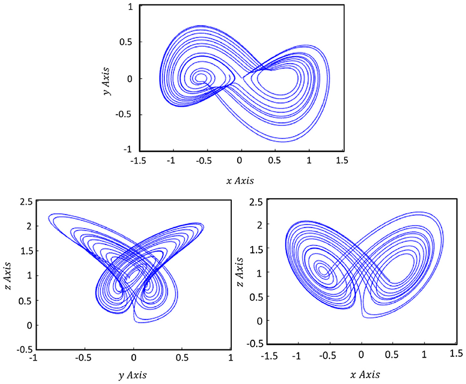
Figure 1. The chaotic attractor of the Shimizu–Morioka dynamical system on the x − y, y − z, and z − x plane, which are shown in the 2D phase portrait for the Master system.

FIGURE 2

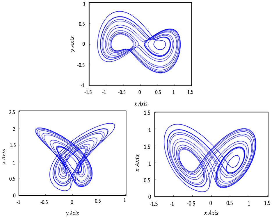
Figure 2. The chaotic attractor of the Shimizu–Morioka dynamical system on the x − y, y − z, and z − x plane, which are shown in the 2D phase portrait for the Drive system.

The times gone by before reaching synchronization states for the Master system (x₁, y₁, z₁) and the Drive system (x₂, y₂, z₂) are shown in Figure 3.

FIGURE 3

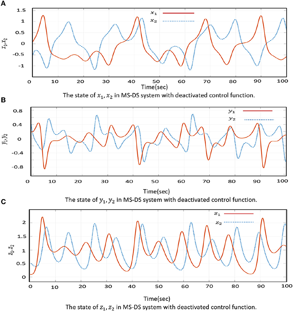
Figure 3. Shown are the states x, y, z before synchronization in dynamical change. (A) The state of x₁, x₂ in MS-DS system with deactivated control function. (B) The state of y₁, y₂ in MS-DS system with deactivated control function. (C) The state of z₁, z₂ in MS-DS system with deactivated control function.

Figure 4 represents the error complexities in the uncontrolled state, while Figures 5, 9 portray the error state behavior in the controlled state.

FIGURE 4

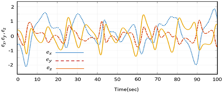
Figure 4. Shown are the error states (e_x, e_y, e_z) before synchronization in dynamical change.

FIGURE 5

Figure 5. Shown are the error states (e_x, e_y, e_z) after synchronization in dynamical change.

3. The general form of the active control approach in master-drive procedure

When MS–DS systems have identical parameters, synchronization via active control is effective. Assume the existence of an (MS–DS) system as

$\begin{array}{ll}ẋ=M_{1}x+g(x)& (2)\end{array}$

$\begin{array}{ll}ẏ=M_{2}y+g(y)+u(t)& (3)\end{array}$

Where $x={(x_1,y_1,...,z_1)}^T\in R^n$ and $y={(x_2,y_2,...,z_2)}^T\in R^n$ are the state vectors of the two systems. $(M_1,M_2)\in R^n\times R^n$ are constant matrix, which designated the coefficient matrix with negative eigenvalues and g(x), g(y) is a sequential nonlinear function and the control function $u(t)=(u_i(t))\in R^n$, which depends on state variables and needs to be calculated where i = (1, 2, ..., n).

Definition:

In some ways, the two equivalent chaotic system (Equations 2, 3) are globally asymptotically synchronized. If a suitable controller u(t) fulfills the condition $\underset{t\to \infty }{lim}\Vert Y(t)-X(t)\Vert$ = $\underset{t\to \infty }{lim}\Vert e_i\Vert$= 0, $\forall e_i(0)\in R^n.$

According to the MS–DS system, scheme (Equations 2, 3) are calculated using the error function defined by e_i = y_i − x_i.

Then, the synchronization error is stated as follows

$\begin{array}{ll}ė=ẏ-ẋ=(M_2-M_1)e+\Gamma (x,y)+u(t)& (4)\end{array}$

Where M₂ − M₁ = M₃ is the coefficient matrix of order (n × n) of the error system (Equation 4) and Γ(x, y) = g(y)−g(x) [47].

Controller u(t) may get rid of the nonlinear section, if system (Equation 4) is not present (e). That is,

$\begin{array}{ll}u(t)=v(t)-\Gamma (x,y)& (5)\end{array}$

Assumption [48]

Control function formulation is defined as follows:

$u=(M_2-M_1)y(t)-(M_2-M_1)x(t)-\Gamma (x,y)+v(t)$

Where $M_2-M_1=M_3\in R^{n\times n}$ is the coefficient matrix of system (Equation 4) [47].

$v(t)=-M_{4}e(t)=-M_4(y(t)-x(t))=-M_{4}e(t)$

Where the linear proposed controller matrix $M_4\in R^{n\times n}$ controls the strength of the master system's controller, which is defined by the subcontroller function v(t).

Since v(t) = −M₄e(t) is a scalar matrix with error variables, by combining (Equations 5, 4) we get

$\begin{array}{ll}ė=M_{3}e+v(t)& (6)\end{array}$

When v(t) is a scalar matrix with error variables and v(t) = −M₄e(t) is a constant matrix, Equation (6) becomes

$\begin{array}{ll}ė=(M_3+M_4)e& (7)\end{array}$

Proposition [47]

λ_i < 0 is the condition for diagonal matrix (M₃ + M₄), where λ_i is the eigenvalue of matrix (M₃ + M₄), state vectors of system (Equation 7) asymptotically converge to zero, and as a result of which MS (Equation 2) tracks the DS (Equation 3).

For M₁ = M₂ and M₁ ≠ M₂, x(t) and y(t) are demonstrated to show the states of two identical and nonidentical chaotic systems. The chaotic synchronization problem can be assumed to be a suitable controller u ∈ Rⁿ, stabilizing the synchronization error at the origin. This indicates that for all t ≥ t₀ ≥ 0, where t₀ is the time of control activation, the controller sends the synchronization error trajectories back to the origin.

3.1. Active control synchronization's effectiveness in the Shimizu–Morioka system

The MS and DS of Shimizu–Morioka systems are defined as follows in this context: The MS of the Shimizu–Morioka system is designated by

$\begin{array}{ll}\begin{array}{c}\dot{x_1}=y_1\hfill \\ \dot{y_1}=x_1-a{y}_1-x_1{z}_1\hfill \\ \dot{z_1}=-b{z}_1+x_1^2\hfill \end{array}\hfill & (8)\end{array}$

The DS of the Shimizu–Morioka system is designated by

$\begin{array}{ll}\begin{array}{c}\dot{x_2}=y_2+u_1\hfill \\ \dot{y_2}=x_2-a{y}_2-x_2{z}_2+u_2\hfill \\ \dot{z_2}=-b{z}_2+x_2^2+u_3\hfill \end{array}\hfill & (9)\end{array}$

In the system (Equation 9), we characterize sequential controllers: u_i(t); ∀u_i = (1, 2, 3) which must be regulated. To estimate the error functions, Equations (8), (9) are subtracted from one another. For the control function obtained, we have to calculate the error state (e_x; ∀x = x, y, z) by combining the DS (Equation 8) and MS systems (Equation 9) using

$\begin{array}{ll}{e}_x=x_2-x_1;e_y=y_2-y_1;e_z=z_2-z_1;\hfill & (10)\end{array}$

Let us derive the error dynamics equations for applying the active control design methods:

$\begin{array}{ll}\begin{array}{c}\dot{e_x}=e_y+u_1\hfill \\ \dot{e_y}=e_x-a{e}_y-x_2{z}_2+x_1{z}_1+u_2\hfill \\ \dot{e_z}=-b{e}_z+e_x(x_2+x_1)+u_3\hfill \end{array}\hfill & (11)\end{array}$

For controlling nonlinearity, the control functions are re-described as (v_i; ∀i = 1, 2, 3) in the system (Equation 12):

$\begin{array}{ll}\begin{array}{c}{v}_1=u_1\hfill \\ v_2=u_2-x_2{z}_2+x_1{z}_1\hfill \\ v_3=u_3\hfill \end{array}\hfill & (12)\end{array}$

The control function (u_i; ∀i = 1, 2, 3) is designated in this formed

$\begin{array}{ll}\begin{array}{c}{u}_1=v_1\hfill \\ u_2=v_2+x_2{z}_2-x_1{z}_1\hfill \\ u_3=v_3\hfill \end{array}\hfill & (13)\end{array}$

The error dynamics system (Equation 11) changes state

$\begin{array}{ll}\begin{array}{c}\dot{e_x}=e_y+v_1\hfill \\ \dot{e_x}=e_x-a{e}_y+v_2\hfill \\ \dot{e_z}=-b{e}_z+e_x(x_2+x_1)+v_3\hfill \end{array}\hfill & (14)\end{array}$

The error variables (e_x; ∀x = x, y, z) are defined by linearizing error system (Equation 11) with control effort (v_i; ∀i = 1, ..., 3). If the control function follows the instructions (e_x; ∀x = x, y, z) → 0 as time (∀ t → ∞), then the system's stabilization is complete. To control the error dynamics (Equation 11) following the active control approach for the control functions (v_i; ∀i = 1, 2, 3), one can use a variety of arbitrary scalar sets to create a constant matrix A, such that

$\begin{array}{ll}{\left[v_1,v_2,v_3\right]}^T=A{\left[e_x,e_y,e_z\right]}^T\hfill & (15)\end{array}$

Where A is a constant matrix. Here, it is examined how the chaotic system's coefficient matrix's eigenvalues [43] influence the results, which are modifiable to get the required synchronization time. To stabilize the error system's state, the matrix A must all have eigenvalues following conditions (λ_i < o). The selection of the matrix is A_i where (i = 1,2,3), in the following procedure:

Case 1. In this case, we take A₁ matrix as follows:

$\begin{array}{c}{A}_1=\left(\begin{array}{ccc}-1& -1& 0\\ -1& -a& 0\\ -\left(x_2+x_1\right)& 0& -b\end{array}\right)\end{array}$

and the control function is

$\begin{array}{ll}\begin{array}{c}{u}_1=-e_x-e_y\hfill \\ u_2=-e_x-a{e}_y+x_2{z}_2-x_1{z}_1\hfill \\ u_3=-(x_2+x_1)e_x-b{e}_z\hfill \end{array}\hfill & (16)\end{array}$

With the corresponding eigenvalues being λ₁ = (−1, −2a, −2b).

Case 2. In this case, we take A₂ matrix as follows:

$\begin{array}{c}{A}_2=\left(\begin{array}{ccc}-a& -1& 0\\ -1& -a-b& 0\\ -\left(x_2+x_1\right)& 0& 0\end{array}\right)\end{array}$

and the control function is

$\begin{array}{ll}\begin{array}{c}{u}_1=-a{e}_x-e_y\hfill \\ u_2=-e_x-(a+b)e_y+x_2{z}_2-x_1{z}_1\hfill \\ u_3=-(x_2+x_1)e_x\hfill \end{array}\hfill & (17)\end{array}$

With the corresponding eigenvalues being λ₂ = (−a, −2a − b, −b).

Case 3. In this case, we take A₃ matrix as follows:

$\begin{array}{c}{A}_3=\left(\begin{array}{ccc}-b& -1& 0\\ -1& -1& 0\\ -\left(x_2+x_1\right)& 0& -1\end{array}\right)\end{array}$

and the control function is

$\begin{array}{ll}\begin{array}{c}{u}_1=-b{e}_x-e_y\hfill \\ u_2=-e_x-e_y+x_2{z}_2-x_1{z}_1\hfill \\ u_3=-(x_2+x_1)e_x-e_z\hfill \end{array}\hfill & (18)\end{array}$

With the corresponding eigenvalues bing λ₃ = (−b, −1−a, −1−b).

Finally, we chose the A₁ matrix for reduced synchronization time in the comparative analysis. Because when we chose A₂ and A₃ matrix for chaos control of Shimizu–Morioka, it takes longer time than A₁ matrix, which is shown in Figures 6A–C.

FIGURE 6

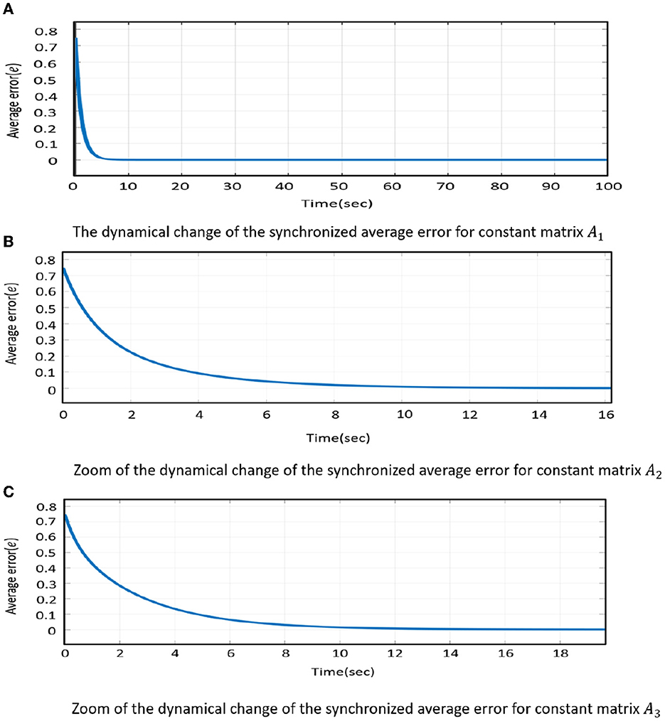
Figure 6. The dynamical change of the synchronized average error when we chose arbitrary matrix (A₁, A₂, A₃) for the control function. (A) To carry out the zoom of the dynamical change of the synchronized average error for constant matrix A₁. (B) Zoom of the dynamical change of the synchronized average error for constant matrix A₂. (C) Zoom of the dynamical change of the synchronized average error for constant matrix A₃.

Now, we prove the control system (Equation 16):

For a given matrix A₁, we can construct the matrix B from the system (Equation 13)

$\begin{array}{c}B=\left(\begin{array}{ccc}0& 1& 0\\ 1& -a& 0\\ \left(x_2+x_1\right)& 0& -b\end{array}\right)\end{array}$

If we fix (Equation 15) into Equation (14), we can explore

$ė=Be+A_{1}e=We$

Where W = (B + A₁) is a diagonal matrix.

$\begin{array}{c}\left(\begin{array}{c}\dot{e_x}\\ \dot{e_y}\\ \dot{e_z}\end{array}\right)=\left(\begin{array}{ccc}0& 1& 0\\ 1& -a& 0\\ \left(x_2+x_1\right)& 0& -b\end{array}\right)\left(\begin{array}{c}{e}_1\\ e_2\\ e_3\end{array}\right)+A_1\left(\begin{array}{c}{e}_1\\ e_2\\ e_3\end{array}\right)\end{array}$

$\begin{array}{c}W=\left(\begin{array}{ccc}-1& 0& 0\\ 0& -2a& 0\\ 0& 0& -2b\end{array}\right)\end{array}$

For this specific selection of constant matrix (A₁; ∀λ₁ = −1, −2a, −2b), according to the linearity system's stability theory, this condition i.e. (e_x; ∀x = x, y, z) → 0 as time (∀ t → ∞), is fulfilled by synchronization laws. As a result, two systems are synchronized under the control system (Equation 20) if all the eigenvalues λ_i of the matrix W satisfy the condition (λ_i < o). From the system (Equation 15) by operating A₁ matrix, we get values of (v₁, v₂, v₃) as follows:

$\begin{array}{ll}\begin{array}{c}{v}_1=-e_x-e_y\hfill \\ v_2=-e_x-a{e}_y\hfill \\ v_3=-(x_2+x_1)e_x-b{e}_z\hfill \end{array}\hfill & (19)\end{array}$

From systems (Equations 13, 19):

$\begin{array}{ll}\begin{array}{c}{u}_1=-e_x-e_y\hfill \\ u_2=-e_x-a{e}_y+x_2{z}_2-x_1{z}_1\hfill \\ u_3=-(x_2+x_1)e_x-b{e}_z\hfill \end{array}\hfill & (20)\end{array}$

3.2. Simulation and results

The MatLab Simulink is applied to the RK-4 algorithm to generate numerical results with a 0.01-time grid. We proceed with the MS (Equation 8) and DS (Equation 9) procedures under the following initial circumstances:

$\begin{array}{ll}{X}_i(0)=(0.1,0.2,0.1);\forall (X=(x,y,z),i=1)\hfill & (21)\end{array}$

and

$\begin{array}{ll}{X}_j(0)=(-0.5,0.4,0.5);\forall (X=(x,y,z),j=2)\hfill & (22)\end{array}$

We used numerical simulations to prove the dynamical change of error states regulated by control functions. Figure 5 represents the error systems (Equation 11) under the controller (Equation 20) for stimulation time t = 100 s; it is apparent that because of activated control signals (e_x; ∀x = x, y, z) → 0 as time (∀ t → ∞). For zero convergence of error states it is necessary to ensure MS (Equation 8) as well as DS (Equation 9) synchronization. To verify the synchronization act, we calculate the synchronization ratio from Figure 6 and we get the average error on the state variables of error dynamics as follows

$e=\sqrt{e_x^2+e_y^2+e_z^2}$

and Figure 7 demonstrates the time history of the synchronization state variables of the MS (Equation 8) and DS (Equation 9) systems, which are (x₁, x₂), (y₁, y₂), and (z₁, z₂) at time t = 0 control signals are activated. Moreover, Figure 8 illustrates the action control's response time from Equation (20) to achieve chaos synchronization between the Master-Drive system. Controllers modify inputs to set the system's output to the desired results. A specific general form of active control and backstepping methods may conduct this control operation [32]. Thus, conclusions contain observations.

FIGURE 7

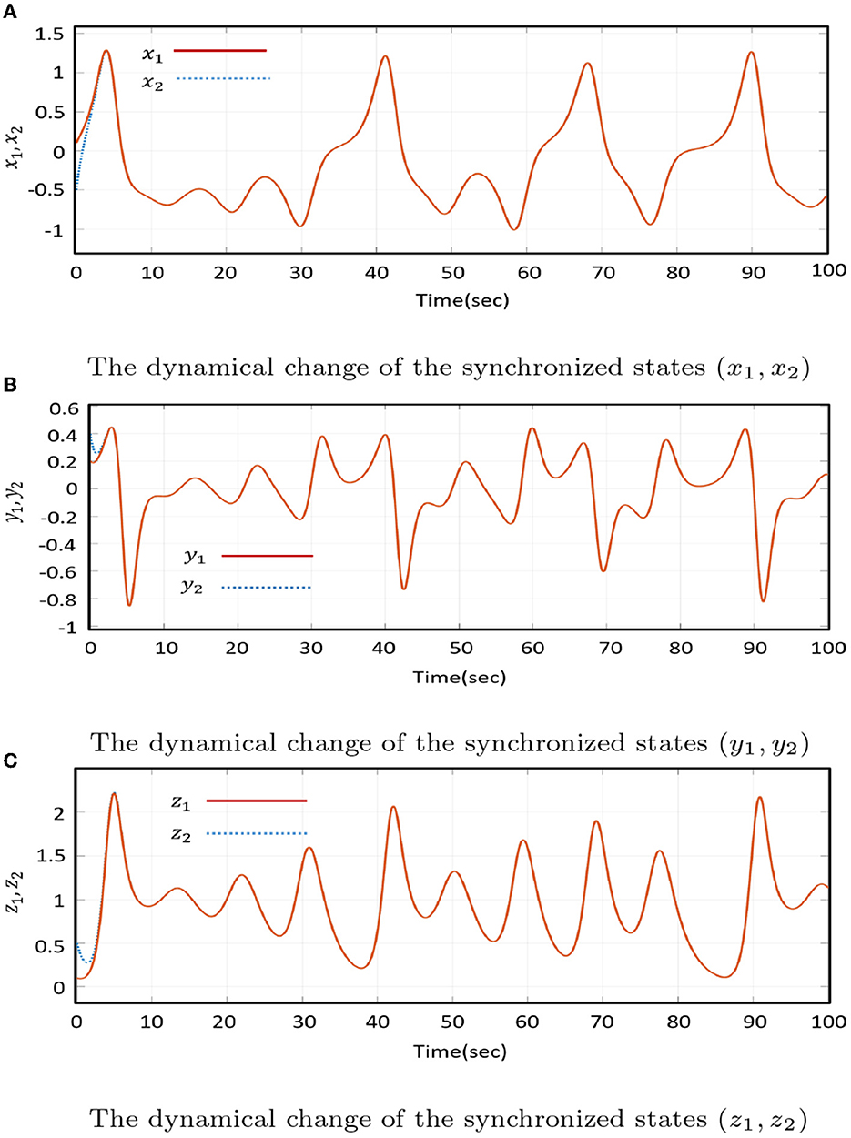
Figure 7. The dynamical change of the states x, y, z after synchronization. (A) The dynamical change of the synchronized states (x₁, x₂). (B) The dynamical change of the synchronized states (y₁, y₂). (C) The dynamical change of the synchronized states (z₁, z₂).

FIGURE 8

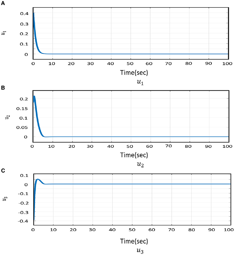
Figure 8. The dynamical change of the synchronized states of control effort u_i. (A) u₁, (B) u₂, and (C) u₃.

The identical chaotic systems exhaust the AC process; the purpose of this section Figure 7 is to depict the time series of the state vectors of the synchronized trajectories. The MS's state trajectories converged to the DS's state trajectories by applying a control effort (Equation 20). The DS system's ability to track the MS system and respective state variables of Equations (8), (9) demonstrate similar behaviors in all upcoming states [49, 50].

4. The general form of the backstepping control approach in master–drive procedure

The backstepping method is regulated by a recursive formulation, which ensures the global asymptotic stability of the system (Equation 23). In the backstepping strategy, Lyapunov's theory is formulated by breaking the proposed model (Equation 24) into a sequence of new system states using subordinate variables of systems (Equation 24). We integrate new variables into the transformation sequence, consisting of the system's subordinate state variables, identical parameters, and stabilizing variables, for creating a control function. By running the sequential step of a model in the backstepping strategy, the Lyapunov function V_m, m = (1, 2, ...n) stabilized the mth subsystem. As soon as ζ_k−1 was designed, the virtual control input ζ_k stabilized the mth equations ∀m ∈ (x, 1, 2, ...k) [5, 51, 52]. A general nonlinear system is formatted as follows [53]:

$\begin{array}{ll}\begin{array}{c}ẋ=f(x)+g(x){\zeta }_1\\ \dot{{\zeta }_1}=u\hfill \end{array}\hfill & (23)\end{array}$

Where ζ₁ ∈ R and x ∈ Rⁿ are the control input and state of the system, and the nonlinear functions are gathered in (f, g). The BC scheme is given as follows to stabilize systems (Equation 24), using the strict feedback form recursively [53]:

$\begin{array}{l}{\dot{e}}_x=f(e_x+g(x,e_x){\zeta }_1\hfill \\ \stackrel{.}{{\zeta }_1}=f_1(x,e_x,{\zeta }_1)+g_1(x,e_x{\zeta }_1){\zeta }_2\hfill \\ \cdots \hfill \\ \stackrel{.}{{\zeta }_{k-1}}=f_{k-1}(x,e_x,{\zeta }_1,\mathrm{...},{\zeta }_{k-1})+g_{k-1}(x,e_x{\zeta }_1,\mathrm{...},{\zeta }_{k-1}){\zeta }_k\hfill \\ \stackrel{.}{{\zeta }_k}=f_k(x,e_x{\zeta }_1,\mathrm{...},{\zeta }_k)+g_k(x,e_x{\zeta }_1,\mathrm{...},{\zeta }_k)u\hfill & (24)\end{array}$

Where e_x, ζ₁, ζ₂, ..., ζ_k are error of state variables and u is the final control function [5].

Step 1:

The stable process of the first of one system (Equation 24) is described as follows:

$\begin{array}{ll}\dot{e_x}=f(x,e_x)+g(x,e_x){\zeta }_1\hfill & (25)\end{array}$

Here, we originate the dynamics state of variable κ₁, which is regulated by κ₁ = e₁ for creating virtual controller ζ₁ under the consideration of Lyapunov functions.

$\dot{{\kappa }_1}=f({\kappa }_1,{\zeta }_1,{\zeta }_2,...,{\zeta }_k)$

Lyapunov function-1:

$V_1({\kappa }_1)=Q{\kappa }_1^T$

Where $Q=\frac{1}{T}>0$. The dynamic change of V₁ is

$\dot{V_1}=f({\kappa }_1^2,{\kappa }_1{\kappa }_2)$

Then, $\dot{V_1}=-Q{\kappa }_1^T<0$ in Rⁿ.

The virtual control ζ₁ = α₁(κ₁) ensures that the system (Equation 25) becomes asymptotically stable by estimating α₁(κ₁), while κ₂ is a controller because of $V_1>0\Rightarrow \dot{V_1}<0$ [44].

Step 2:

The stable process of the second of one system (Equation 24) is described as follows:

$\begin{array}{ll}\dot{{\zeta }_1}=f_1(x,{\zeta }_1)+g_1(x,{\zeta }_1){\zeta }_2\hfill & (26)\end{array}$

The new virtual variable κ₂ is defined by ζ₁ and α₁(z₁) as:

$\begin{array}{ll}{\kappa }_2={\zeta }_1-{\alpha }_1({\kappa }_1)\hfill & (27)\end{array}$

Now, let us consider that the $\dot{{\kappa }_1},\dot{{\kappa }_2}$ are subordinate coordinates of a new error subsystem:

$\begin{array}{ll}\begin{array}{c}\dot{{\kappa }_1}=f({\kappa }_1,{\zeta }_1,{\zeta }_2,...,{\zeta }_k)\hfill \\ \dot{{\kappa }_2}=f({\kappa }_1,{\kappa }_2,{\zeta }_2,...,{\zeta }_k)-\dot{{\alpha }_1}({\kappa }_1)\hfill \end{array}\hfill & (28)\end{array}$

Lyapunov function-2:

$V_2({\kappa }_1,{\kappa }_2)=V_1({\kappa }_1)+Q{\kappa }_2^T$

Therefore, the dynamical change of V₂ is:

$\dot{V_2}=f({\kappa }_1^2,{\kappa }_2^2,{\kappa }_2{\kappa }_3)$

Then, $\dot{V_2}=-Q{\kappa }_1^T-Q{\kappa }_2^T<0$ in Rⁿ.

While κ₃ is a controller, the virtual control ζ₂ = α₂(κ₁, κ₂) ensures that the system labeled (Equation 26) is asymptotically stable by estimating α₂(κ₁, κ₂).

Step n:

The ongoing dimensional step defines the error variable κ_n:

$\begin{array}{ll}{\kappa }_n={\zeta }_k-{\alpha }_{n-1}({\kappa }_1,{\kappa }_2,{\kappa }_3,...,{\kappa }_n)\hfill & (29)\end{array}$

The new virtual variable subsystems are given as follows:

$\begin{array}{ll}\begin{array}{c}\dot{{\kappa }_1}=f({\kappa }_1,{\zeta }_1,{\zeta }_2,...,{\zeta }_k)\hfill \\ \dot{{\kappa }_2}=f({\kappa }_1,{\kappa }_2,{\zeta }_2,...,{\zeta }_k)-\dot{{\alpha }_1}({\kappa }_1)\hfill \\ \dot{{\kappa }_3}=f({\kappa }_1,{\kappa }_2,{\kappa }_3,{\zeta }_3,...,{\zeta }_k)-\dot{{\alpha }_2}({\kappa }_1,{\kappa }_2)\hfill \\ \cdots \hfill \\ \cdots \hfill \\ \dot{{\kappa }_n}=f({\kappa }_1,{\kappa }_2,{\kappa }_3,...,{\kappa }_n)-\dot{{\alpha }_{n-1}}({\kappa }_1,{\kappa }_2,\kappa {\kappa }_3,...,{\kappa }_n)+u\hfill \end{array}\hfill & (30)\end{array}$

Lyapunov function-n:

$V_n({\kappa }_1,{\kappa }_2,{\kappa }_3,...,{\kappa }_n)=V_{n-1}({\kappa }_1,{\kappa }_2,{\kappa }_3,...,{\kappa }_{n-1})+Q{\kappa }_n^T$

Hence, the dynamical change of V_n is:

$\dot{V_n}=f({\kappa }_1^2,{\kappa }_2^2,{\kappa }_3,...,{\kappa }_{n-1}{\kappa }_n)$

Then, $\dot{V_1}=-Q_1{\kappa }_1^T-Q_2{\kappa }_2^T-...-Q_n{\kappa }_n^T<0$ in Rⁿ, where $Q_i=T^{-1},\forall (i=1,\cdots ,n)>0$, and T > 0 which are scalars. According to the Lyapunov stability theory, the subsystem (Equation 29) is asymptotically stable when $\dot{V_2}=-Q{\kappa }_1^T-Q{\kappa }_2^T<0$. While u is a controller, the virtual control α_n−1(κ₁, κ₂, κ₃, ..., κ_n) ensures that the whole system (Equation 24) is asymptotically stable by estimating α_n−1(κ₁, κ₂, κ₃, ..., κ_n), which generally depends on x and ζ₁, ζ₂, ..., ζ_k, is gradually accomplished in n steps. As a result of the previous procedures, the system (Equation 23) is enormously stable worldwide for all initial conditions $x_i(0)\in R^n$.

4.1. Backstepping control synchronization's effectiveness in the Shimizu–Morioka system

The MS of the Shimizu–Morioka systems:

$\begin{array}{ll}\begin{array}{c}\dot{x_1}=y_1\hfill \\ \dot{y_1}=x_1-a{y}_1-x_1{z}_1\hfill \\ \dot{z_1}=-b{z}_1+x_1^2\hfill \end{array}\hfill & (31)\end{array}$

is given in terms of the DS as

$\begin{array}{ll}\begin{array}{c}\dot{x_2}=y_2\hfill \\ \dot{y_2}=x_2-a{y}_2-x_2{z}_2+u\hfill \\ \dot{z_2}=-b{z}_2+x_2^2\hfill \end{array}\hfill & (32)\end{array}$

Here, u is a single control input to be identified subsequently. We originated the error system concerning time for applying the backstepping control strategy using the error states, explanation (Equation 10) by combining (Equations 31, 32).

$\begin{array}{ll}\begin{array}{c}\dot{e_x}=e_y\hfill \\ \dot{e_y}=e_x-a{e}_y-x_2{z}_2+x_1{z}_1+u\hfill \\ \dot{e_z}=-b{e}_z+e_x(x_2+x_1)\hfill \end{array}\hfill & (33)\end{array}$

Following the sequence of the entire systems (Equation 24), the error system (Equation 33) is mentioned previously as:

$\begin{array}{ll}\begin{array}{c}\dot{e_z}=-b{e}_z+e_x(x_2+x_1)\hfill \\ \dot{e_x}=e_y\hfill \\ \dot{e_y}=e_x(1-z_2)-a{e}_y-x_1{e}_z+u\hfill \end{array}\hfill & (34)\end{array}$

This project designated as control input u to ensure the stability of the error system (Equation 34). According to Section 4, the 3D nonlinear chaotic system will be governed by a three-step recursive strategy. To simplify the system (Equation 34), we divided it into three smaller units, each of which included a single virtual control function and a virtual variable. The formulation continues following the sequential equation of the system (Equation 34) from the first to the last subsystem until the transformation of the coordinates from $(\dot{e_x},\dot{e_y},\dot{e_z})$ to $(\dot{{\kappa }_1},\dot{{\kappa }_2},\dot{{\kappa }_3})$.

Step-1:

When e_z is a controller and the first Lyapunov function is defined by a new virtual variable κ₁ = e_z, for creating the virtual control α₁, which ensures that the first equation of Equation (34) is asymptotically stable by estimating the virtual control α₁. The purpose of controller e_z is to drive (e_x, e_y, e_z) = (0, 0, 0) i.e. (x₁; y₁; z₁) = (x₂; y₂; z₂). Lyapunov function [44]-1:

$\begin{array}{ll}{V}_1({\kappa }_1)=\frac{1}{2}{({\kappa }_1)}^2\hfill & (35)\end{array}$

$\dot{V_1}$ is regulated by $\dot{{\kappa }_1}$ in the following ways:

$\dot{V_1}={\kappa }_1\dot{{\kappa }_1}={\kappa }_1(-b{e}_z+e_x(x_2+x_1))$

When e_x = α₁(e_z) is used to define the second new virtual variable κ₂ = e_x − α₁, we obtain

$\begin{array}{ll}\begin{array}{c}\dot{V_1}={\kappa }_1(-b{e}_z+({\kappa }_2+{\alpha }_1)(x_2+x_1))\hfill \\ \dot{V_1}=-b{({\kappa }_1)}^2+{\kappa }_1{\kappa }_2(x_2+x_1)+{\kappa }_1(x_2+x_1){\alpha }_1\hfill \end{array}\hfill & (36)\end{array}$

There exists α₁ = 0,

$\begin{array}{ll}\dot{V_1}=-b{({\kappa }_1)}^2+{\kappa }_1{\kappa }_2(x_2+x_1)\hfill & (37)\end{array}$

Consequently, $\dot{V_1}<0$. In the following step, the term κ₁κ₂(x₂ + x₁) in Equation (37) will be eliminated.

Step-2:

The second virtual variable is governed by the system's (Equation 34) second equation, in which α₁ = 0 exists.

$\dot{{\kappa }_2}=\dot{e_x}-\dot{{\alpha }_1}$

$\dot{{\kappa }_2}=e_y$

When e_y is a controller and the second Lyapunov function is defined by the new virtual variable κ₃ = e_y − α₂. We derived stabilization function α₂, which ensures that the second of Equation (34) is asymptotically stable, by estimating α₂.

Lyapunov function-2:

$\begin{array}{ll}\begin{array}{c}{V}_2({\kappa }_1,{\kappa }_2)=V_1({\kappa }_1)+\frac{1}{2}{({\kappa }_2)}^2\\ \dot{V_2}=\dot{V_1}(e_z)+{\kappa }_2\dot{{\kappa }_2}\hfill \end{array}\hfill & (38)\end{array}$

When we use the time derivative of κ₂ in $\dot{V_2}$, then the dynamical change of V₂ takes place as follows::

$\begin{array}{ll}\begin{array}{c}\dot{V_2}=\dot{V_1}(e_z)+{\kappa }_2{e}_y\hfill \\ \dot{V_2}=-b{({\kappa }_1)}^2+{\kappa }_1{\kappa }_2(x_2+x_1)+{\kappa }_2({\kappa }_3+{\alpha }_2)\hfill \\ \dot{V_2}=-b{\kappa }_1^2-{\kappa }_2^2+{\kappa }_2{\kappa }_3+{\kappa }_2({\kappa }_2+{\kappa }_1(x_2+x_1)+{\alpha }_2)\hfill \end{array}\hfill & (39)\end{array}$

The stabilization function α₂ is chosen as:

$\begin{array}{ll}{\alpha }_2=-{\kappa }_2-{\kappa }_1(x_2+x_1)\hfill & (40)\end{array}$

Furthermore by substituting ${\alpha }_2,\dot{V_2}$ gets converted into:

$\begin{array}{ll}\dot{V_2}=-b{\kappa }_1^2-{\kappa }_2^2+{\kappa }_2{\kappa }_3\hfill & (41)\end{array}$

In light of this, $\dot{V_1}<0$. In the following step, the term κ₂κ₃ from Equation (41) will be eliminated.

Assumption

If we follow the sequence of Equation (30) and the control effort exists in the third equation, then we get

${\alpha }_2=\frac{{\kappa }_1+e_x(1-z_2)-(a-1){\alpha }_1}{x_1}$

If

${\alpha }_2=\frac{f(x,e_x,{\kappa }_1)}{x}$

Then, the solution of state variable (x, y, z) → ∞

Step-3:

The third virtual variable is governed by the third equation of systems (Equation 34), in which α₂ = −κ₂−κ₁(x₂ + x₁) exists. The third virtual variable is now:

$\dot{{\kappa }_3}=\dot{e_y}-\dot{{\alpha }_2}$

$\begin{array}{ll}\dot{{\kappa }_3}=-b{e}_x(1-z_2)-a{e}_y-x_1{e}_z+u-\dot{{\alpha }_2}\hfill & (42)\end{array}$

Lyapunov function-3:

$\begin{array}{rr}\hfill \begin{array}{c}\hfill V_3({\kappa }_2,{\kappa }_3)=V_2({\kappa }_2)+\frac{1}{2}{({\kappa }_3)}^2\\ \dot{V_3}(e_z,{\kappa }_2,{\kappa }_3)=\dot{V_2}(e_z,{\kappa }_2)+{\kappa }_3\dot{{\kappa }_3}\hfill \end{array}& (43)\end{array}$

$\dot{V_3}$ is regulated by $\dot{{\kappa }_3}$ in the following ways:

$\begin{array}{l}\stackrel{.}{V_3}=-b{\kappa }_1^2-{\kappa }_2^2+{\kappa }_2{\kappa }_3+{\kappa }_3\stackrel{.}{{\kappa }_3}\hfill \\ \stackrel{.}{V_3}=-b{\kappa }_1^2-{\kappa }_2^2+{\kappa }_2{\kappa }_3+{\kappa }_3[-b{e}_x(1-z_2)\hfill \\ -a{e}_y-x_1{e}_z+u-\stackrel{.}{{\alpha }_2}]\hfill \\ \stackrel{.}{V_3}=-b{\kappa }_1^2-{\kappa }_2^2-a{\kappa }_3^2+{\kappa }_3({\kappa }_2-a{\alpha }_2+(1-z_2)\hfill \\ e_x-x_1{e}_z-\stackrel{.}{{\alpha }_2}+u)\hfill & (44)\end{array}$

If the following preference for the control variable u:

$\begin{array}{ll}u=-{\kappa }_2+a{\alpha }_2-(1-z_2)e_x+x_1{e}_z+\dot{{\alpha }_2}\hfill & (45)\end{array}$

so that,

$\dot{V_3}=-b{\kappa }_1^2-{\kappa }_2^2-a{\kappa }_3^2<0$

(i.e., $\dot{V_3<0}$, since a, b > 0) and according to the LaSalle-Yoshizawa theorem [16, 54], it is necessary to make it clear that all solutions of Equation (34) satisfy the conditions (e_x; ∀x = x, y, z) → 0 as time (∀ t → ∞). Thus, systems (Equations 31, 32) are globally synchronized with the control function u. Furthermore, the set of new virtual variables is a new error model shown in (κ₁, κ₂, κ₃) coordinates in Equation (46), and now let us analyze the entire space of $(\dot{{\kappa }_1},\dot{{\kappa }_2},\dot{{\kappa }_3})$ :

$\begin{array}{ll}\begin{array}{c}\dot{{\kappa }_1}=-b{\kappa }_1+e_x(x_2+x_1)\hfill \\ \dot{{\kappa }_2}=e_y\hfill \\ \dot{{\kappa }_3}=e_x(1-z_2)-a{e}_y-x_1{e}_z+u-\dot{{\alpha }_2}\hfill \end{array}\hfill & (46)\end{array}$

4.2. Simulation and results

The MatLab Simulink is applied to the RK-4 algorithm to generate numerical results with a 0.01-time grid. We proceed with the system (Equation 34) for completing the backstepping design simulation procedures under controller (Equation 45). Now, we proceed with fixing the parameter values of a = 0.81, b = 0.375, as shown in Figures 9–14, where initial circumstances:

$\begin{array}{ll}{X}_i(0)=(0.1,0.2,0.1);\forall (X=(x,y,z),i=1)\hfill & (47)\end{array}$

and

$\begin{array}{ll}{X}_j(0)=(-0.5,0.4,0.5);\forall (X=(x,y,z),j=2)\hfill & (48)\end{array}$

FIGURE 9

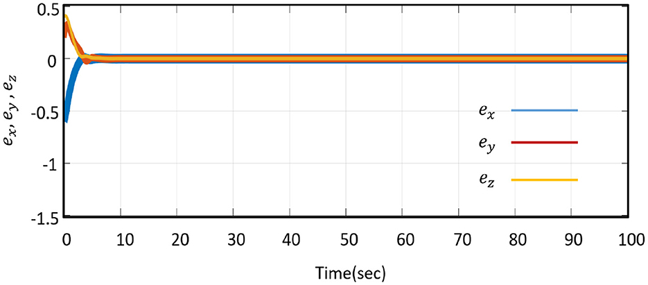
Figure 9. Tracking error e_x, e_y, e_z.

FIGURE 10

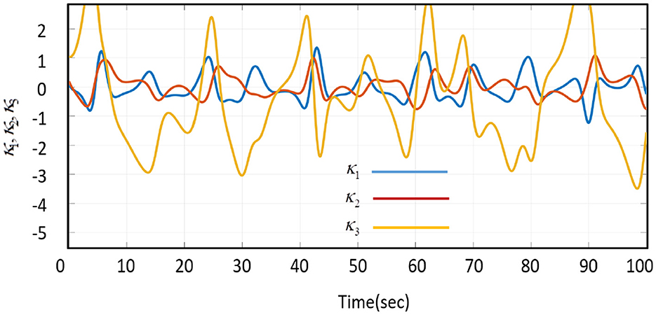
Figure 10. The error model with a virtual variable for backstepping without activated control.

FIGURE 11

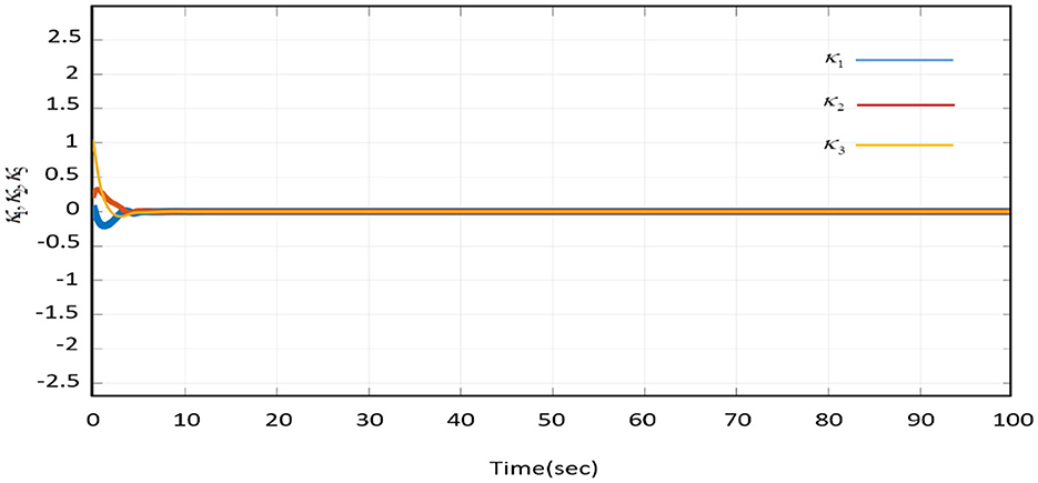
Figure 11. The error model with the virtual variable for backstepping with activated control.

FIGURE 12

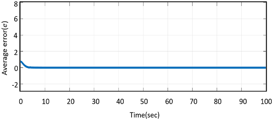
Figure 12. Average error e.

FIGURE 13

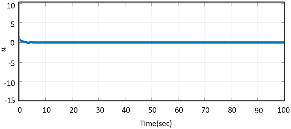
Figure 13. Control effort u.

FIGURE 14

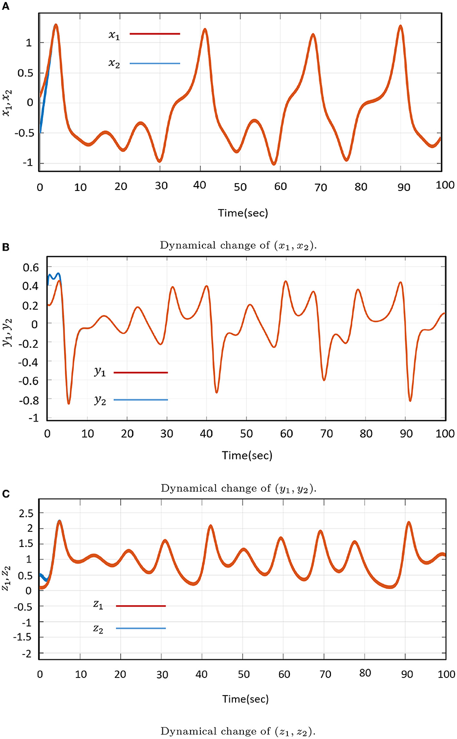
Figure 14. Dynamical change of the states x, y, z after synchronization. (A) Dynamical change of (x₁, x₂). (B) Dynamical change of (y₁, y₂). (C) Dynamical change of (z₁, z₂).

The dynamical change of error state (e_x, e_y, e_z) and new subsystem (κ₁, κ₂, κ₃) with activated control function is shown in Figures 9–14.

The validity of a new subsystem under backstepping control with system equilibrium (0, 0, 0) is examined in Figure 12, along with the magnitude of system synchronization (Equation 34). According to Equation (34), the average error propagation is calculated as follows:

$e=\sqrt{e_x^2+e_y^2+e_z^2}$

The MS–DS system is globally synchronized following an initial momentary time period of approximately t = 2.5s. This is also supported by Figure 15B, where the exponential convergence of the synchronization superiority is determined by the error propagation on average error states:

FIGURE 15

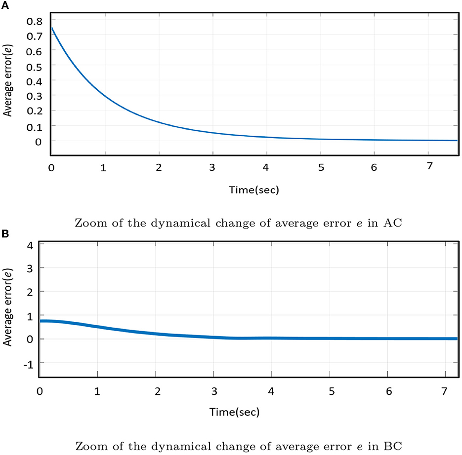
Figure 15. Effectiveness of the synchronization times for (A) the AC approach and (B) the BC approach with the controller turned on for (0 ≤ t ≤ 100).

Figure 15 shows the time response of the control law.

Figure 14 shows the synchronized states of MS–DS of the Shimizu–Morioka system devastating BC process by the activated controller. Thus, it is necessary the effectiveness of the DS is necessary to track the MS with similar characteristics for all future states.

5. Comparing AC and BC strategies

Figures 15A, B demonstrate edge comparisons of the effects of two different approaches on the synchronization time of a given identical MS–DS Shimizu–Morioka chaotic system. Average error (e) is utilized to dynamically analyze the synchronization excellence when the control function is stimulated at t = 0, as shown in Figure 15. At t ≥ 2.5, the control is given by the backstepping controller; however, at t ≥ 4.5, active controllers are used to observe the E₀(0, 0, 0) equilibrium point with a 2 s time delay [55–57]. It can be determined that the backstepping design is more successful in achieving control of the Shimizu–Morioka chaotic system by comparing the active control and backstepping strategy procedures at the same particular time [58]. In AC and BC control, a 3-dimensional autonomous system, the BC formula reduces the number of controllers from 3 to 1, and active control work sequentially. As a result, backstepping control outperforms the active control, thereby reducing controller complexity and cost.

6. Conclusion

This article demonstrates how a single controller operating in a backstepping and following a sequential controller for active control can easily control chaos in a Shimizu–Morioka chaotic system. All theoretical analyzes are validated using simulation results. Furthermore, numerical simulations are used to compare the performance of the projected control approaches. We have shown that the backstepping controller regulates the control of the Shimizu–Morioka chaotic system better than the active controllers, which represents the effectiveness of the backstepping control method. The effects of the two techniques are represented graphically together with a time history (Figures 1–14). Listed are the descriptions:

• The active control design includes sequential controllers and the backstepping design creates one controller by defining the Lyapunov function.

• In both methods, the error dynamic is the tendency toward zero as time goes to infinity, hence the chaos synchronization of the Shimizu-Morioka chaotic system is asymptotically stable.

• The states of MS (master system) and DS (drive system) exhibit similar activities in both instructions.

• The results demonstrated that tracking the backstepping strategy takes much less time than the active control method for detecting the dynamics of transitory errors. Backstepping only needs one controller, and in a few steps, it reaches global stability and asymptotic synchronization. Backstepping outperforms other strategies and is simpler to design.

Data availability statement

The original contributions presented in the study are included in the article/supplementary material, further inquiries can be directed to the corresponding author.

Author contributions

AT: manuscript writing, methodology, and software. MA: overview of the article and methodology. All authors contributed to the article and approved the submitted version.

Conflict of interest

The authors declare that the research was conducted in the absence of any commercial or financial relationships that could be construed as a potential conflict of nterest.

Publisher's note

All claims expressed in this article are solely those of the authors and do not necessarily represent those of their affiliated organizations, or those of the publisher, the editors and the reviewers. Any product that may be evaluated in this article, or claim that may be made by its manufacturer, is not guaranteed or endorsed by the publisher.

References

1. Alligood KT, Sauer TD, Yorke JA. Chaos. Berlin; Heidelberg: Springer (1996).

Google Scholar

2. Peng CC, Hsue AWJ, Chen CL. Variable structure based robust backstepping controller design for nonlinear systems. Nonlinear Dynaics. (2011) 63:253–62. doi: 10.1007/s11071-010-9801-8

PubMed Abstract | CrossRef Full Text | Google Scholar

3. Elabbasy E, Agiza H, El-Dessoky M. Global chaos synchronization for four-scroll attractor by nonlinear control. Sci Res Essays. (2006) 1:065–071.

Google Scholar

4. Uçar A, Lonngren KE, Bai EW. Synchronization of chaotic behavior in nonlinear Bloch equations. Phys Lett A. (2003) 314:96–101. doi: 10.1016/S0375-9601(03)00864-8

CrossRef Full Text | Google Scholar

5. Krstic M, Kokotovic PV, Kanellakopoulos I. Nonlinear and Adaptive Control Design. New York, NY: John Wiley & Sons Inc (1995).

Google Scholar

6. Zhang H, Chen D, Xu B, Wang F. Nonlinear modeling and dynamic analysis of hydro-turbine governing system in the process of load rejection transient. Energy Convers Manag. (2015) 90:128–37. doi: 10.1016/j.enconman.2014.11.020

CrossRef Full Text | Google Scholar

7. Njah A. Tracking control and synchronization of the new hyperchaotic Liu system via backstepping techniques. Nonlinear Dyn. (2010) 61:1–9. doi: 10.1007/s11071-009-9626-5

CrossRef Full Text | Google Scholar

8. Yan Z. Chaos Q-S synchronization between Rössler system and the new unified chaotic system. Phys Lett A. (2005) 334:406–12. doi: 10.1016/j.physleta.2004.11.042

CrossRef Full Text | Google Scholar

9. Wu X, Wang H. A new chaotic system with fractional order and its projective synchronization. Nonlinear Dyn. (2010) 61:407–17. doi: 10.1007/s11071-010-9658-x

PubMed Abstract | CrossRef Full Text | Google Scholar

10. An H, Chen Y. The function cascade synchronization method and applications. Commun Nonlinear Sci Numer Simula. (2008) 13:2246–55. doi: 10.1016/j.cnsns.2007.05.029

CrossRef Full Text | Google Scholar

11. Azar AT, Vaidyanathan S, Ouannas A. Fractional Order Control and Synchronization of Chaotic Systems, Vol. 688. Cham: Springer (2017).

Google Scholar

12. Lungu M. Control of double gimbal control moment gyro systems using the backstepping control method and a nonlinear disturbance observer. Acta Astronautica. (2021) 180:639–49. doi: 10.1016/j.actaastro.2020.10.040

CrossRef Full Text | Google Scholar

13. Olusola OI, Vincent E, Njah AN, Ali E. Control and synchronization of chaos in biological systems via backsteping design. Int J Nonlinear Sci. (2011) 11:121–8.

PubMed Abstract | Google Scholar

14. Fadhel FS, Noaman SF. The generalized backstepping control method for stabilizing and solving systems of multiple delay differential equations. Al-Nahrain J Sci. (2018) 1:150–6. doi: 10.22401/ANJS.00.1.20

CrossRef Full Text | Google Scholar

15. Ai W, Chen W, Hua S. Distributed cooperative learning for a group of uncertain systems via output feedback and neural networks. J Franklin Inst. (2018) 355:2536–61. doi: 10.1016/j.jfranklin.2018.01.030

CrossRef Full Text | Google Scholar

16. Yao Q. Synchronization of second-order chaotic systems with uncertainties and disturbances using fixed-time adaptive sliding mode control. Chaos Solitons Fractals. (2021) 142:110372. doi: 10.1016/j.chaos.2020.110372

CrossRef Full Text | Google Scholar

17. Onma O, Olusola O, Njah A. Control and synchronization of chaotic and hyperchaotic Lorenz systems via extended backstepping techniques. J Nonlinear Dyn. (2014) 2014:861727. doi: 10.1155/2014/861727

CrossRef Full Text | Google Scholar

18. Yassen M. Controlling chaos and synchronization for new chaotic system using linear feedback control. Chaos Solitons Fractals. (2005) 26:913–20. doi: 10.1016/j.chaos.2005.01.047

CrossRef Full Text | Google Scholar

19. Benachour S, Shiromoto HS, Andrieu V. Locally optimal controllers and globally inverse optimal controllers. Automatica. (2014) 50:2918–23. doi: 10.1016/j.automatica.2014.10.019

CrossRef Full Text | Google Scholar

20. Hamiche H, Kemih K, Ghanes M, Zhang G, Djennoune S. Passive and impulsive synchronization of a new four-dimensional chaotic system. Nonlinear Anal Theory Methods Appl. (2011) 74:1146–54. doi: 10.1016/j.na.2010.09.051

CrossRef Full Text | Google Scholar

21. Pecora LM, Carroll TL. Synchronization in chaotic systems. Phys Rev Lett. (1990) 64:821. doi: 10.1103/PhysRevLett.64.821

PubMed Abstract | CrossRef Full Text | Google Scholar

22. Pecora LM, Carroll TL. Driving systems with chaotic signals. Phys Rev A. (1991) 44:2374. doi: 10.1103/PhysRevA.44.2374

PubMed Abstract | CrossRef Full Text | Google Scholar

23. Lorenz EN. Deterministic nonperiodic flow. J Atmosphere Sci. (1963) 20:130–41. doi: 10.1175/1520-0469(1963)020<0130:DNF>2.0.CO;2

CrossRef Full Text | Google Scholar

24. Changaival B, Rosalie M. Exploring chaotic dynamics by partition of bifurcation diagram. In: Workshop on Advance in Nonlinear Complex Systems and Applications (WANCSA). (2017).

PubMed Abstract | Google Scholar

25. Njitacke Z, foz in T, Kengne LK, Leutcho G, Kengne EM, Kengne J. Multistability and its annihilation in the chua's oscillator with piecewise-linear nonlinearity. Chaos Theory Appl. (2020) 2:77–89.

Google Scholar

26. Njitacke ZT, Kengne J. Nonlinear dynamics of three-neurons-based Hopfield neural networks (HNNs): Remerging Feigenbaum trees, coexisting bifurcations and multiple attractors. J Circ Syst Comput. (2019) 28:1950121. doi: 10.1142/S0218126619501214

CrossRef Full Text | Google Scholar

27. Shil'nikov AL. On bifurcations of the Lorenz attractor in the Shimizu-Morioka model. Physica D. (1993) 62:338–346. doi: 10.1016/0167-2789(93)90292-9

CrossRef Full Text | Google Scholar

28. El-Dessoky M, Yassen M, Aly E. Bifurcation analysis and chaos control in Shimizu-Morioka chaotic system with delayed feedback. Appl Math Comput. (2014) 243:283–97. doi: 10.1016/j.amc.2014.05.072

CrossRef Full Text | Google Scholar

29. Kocamaz UE, Uyaroğlu Y, Vaidyanathan S. Control of Shimizu-Morioka chaotic system with passive control, sliding mode control and backstepping design methods: a comparative analysis. In: Vaidyanathan S, Volos C, editors. Advances and Applications in Chaotic Systems. Cham: Springer (2016). p. 409–25.

Google Scholar

30. Codreanu S. Synchronization of spatiotemporal nonlinear dynamical systems by an active control. Chaos Solitons Fractals. (2003) 15:507–10. doi: 10.1016/S0960-0779(02)00128-5

CrossRef Full Text | Google Scholar

31. Bai EW, Lonngren KE. Synchronization of two Lorenz systems using active control. Chaos Solitons Fractals. (1997) 8:51–8. doi: 10.1016/S0960-0779(96)00060-4

PubMed Abstract | CrossRef Full Text | Google Scholar

32. Soong T. Introduction to Active Control. Vienna: Springer (1994).

Google Scholar

33. Mathiyalagan K, Park JH, Sakthivel R. Synchronization for delayed memristive BAM neural networks using impulsive control with random nonlinearities. Appl Math Comput. (2015) 259:967–79. doi: 10.1016/j.amc.2015.03.022

CrossRef Full Text | Google Scholar

34. Mathiyalagan K, Anbuvithya R, Sakthivel R, Park JH, Prakash P. Non-fragile H∞ synchronization of memristor-based neural networks using passivity theory. Neural Networks. (2016) 74:85–100. doi: 10.1016/j.neunet.2015.11.005

PubMed Abstract | CrossRef Full Text | Google Scholar

35. Fu Q, Cai J, Zhong S, Yu Y. Pinning impulsive synchronization of stochastic memristor-based neural networks with time-varying delays. Int J Control Automat Syst. (2019) 17:243–52. doi: 10.1007/s12555-018-0295-3

CrossRef Full Text | Google Scholar

36. Vincent U. Chaos synchronization using active control and backstepping control: a comparative analysis. Nonlinear Anal Model Control. (2008) 13:253–61. doi: 10.15388/NA.2008.13.2.14583

CrossRef Full Text | Google Scholar

37. Yassen M. Chaos control of chaotic dynamical systems using backstepping design. Chaos Solitons Fractals. (2006) 27:537–48. doi: 10.1016/j.chaos.2005.03.046

CrossRef Full Text | Google Scholar

38. Tan X, Zhang J, Yang Y. Synchronizing chaotic systems using backstepping design. Chaos Solitons Fractals. (2003) 16:37–45. doi: 10.1016/S0960-0779(02)00153-4

CrossRef Full Text | Google Scholar

39. Guan H, Zhao D, Wang Y, Yu P. Adaptive anti-synchronization of Cai chaotic systems with fully unknown parameters. In: 2010 International Workshop on Chaos-Fractal Theories and Applications. Kunming: IEEE (2010). p. 53–6.

Google Scholar

40. Al-Sawalha MM, Noorani M, Al-Dlalah M. Adaptive anti-synchronization of chaotic systems with fully unknown parameters. Comput Math Appl. (2010) 59:3234–44. doi: 10.1016/j.camwa.2010.03.010

CrossRef Full Text | Google Scholar

41. Munoz LE, Santos O, Castillo P. Robust nonlinear real-time control strategy to stabilize a PVTOL aircraft in crosswind. In: 2010 IEEE/RSJ International Conference on Intelligent Robots and Systems. Taipei: IEEE (2010). p. 1606–11.

Google Scholar

42. Singh JP, Singh PP, Roy BK. Hybrid synchronization of lu and bhalekar-gejji chaotic systems using nonlinear active control. IFAC Proc Volumes. (2014) 47:292–6. doi: 10.3182/20140313-3-IN-3024.00069

CrossRef Full Text | Google Scholar

43. Ho MC, Hung YC, Chou CH. Phase and anti-phase synchronization of two chaotic systems by using active control. Phys Lett A. (2002) 296:43–8. doi: 10.1016/S0375-9601(02)00074-9

CrossRef Full Text | Google Scholar

44. Jankovic M, Sepulchre R, Kokotovic PV. Constructive Lyapunov stabilization of nonlinear cascade systems. IEEE Trans Autom Control. (1996) 41:1723–35. doi: 10.1109/9.545712

CrossRef Full Text | Google Scholar

45. Nishad C, Prasad R, Kumar P. Synchronization Analysis Chaos of Fractional Derivatives Chaotic Satellite Systems via Feedback Active Control Methods. Authorea [Preprint]. (2022). doi: 10.22541/au.165527106.69915094/v1

CrossRef Full Text | Google Scholar

46. Salih RH. The stability analysis of the shimizu-morioka system with Hopf bifurcation. J Kirkuk Univer Sci Stud. (2011) 6:43161. doi: 10.32894/kujss.2011.43161

CrossRef Full Text | Google Scholar

47. Lei Y, Xu W, Xie W. Synchronization of two chaotic four-dimensional systems using active control. Chaos Solitons Fractals. (2007) 32:1823–9. doi: 10.1016/j.chaos.2005.12.014

CrossRef Full Text | Google Scholar

48. Ahmad I, Saaban AB, Ibrahim AB, Shahzad M. A research on active control to synchronize a new 3D chaotic system. Systems. (2015) 4:2. doi: 10.3390/systems4010002

PubMed Abstract | CrossRef Full Text | Google Scholar

49. Vincent U. Synchronization of identical and non-identical 4-D chaotic systems using active control. Chaos Solitons Fractals. (2008) 37:1065–75. doi: 10.1016/j.chaos.2006.10.005

CrossRef Full Text | Google Scholar

50. Njah A, Vincent U. Chaos synchronization between single and double wells Duffing-Van der Pol oscillators using active control. Chaos Solitons Fractals. (2008) 37:1356–61. doi: 10.1016/j.chaos.2006.10.038

CrossRef Full Text | Google Scholar

51. Khalil HK. Adaptive output feedback control of nonlinear systems represented by input-output models. IEEE Trans Autom Control. (1996) 41:177–88. doi: 10.1109/9.481517

PubMed Abstract | CrossRef Full Text | Google Scholar

52. Yang T, Li XF, Shao HH. Chaotic synchronization using backstepping method with application to the Chua's circuit and Lorenz system. In: Proceedings of the 2001 American Control Conference.(Cat. No. 01CH37148). Vol. 3. Arlington, VA: IEEE (2001). p. 2299–300.

Google Scholar

53. Vaidyanathan S, Azar AT. Backstepping Control of Nonlinear Dynamical Systems. Academic Press (2020).

Google Scholar

54. Yan JJ, Yang YS, Chiang TY, Chen CY. Robust synchronization of unified chaotic systems via sliding mode control. Chaos Solitons Fractals. (2007) 34:947–54. doi: 10.1016/j.chaos.2006.04.003

CrossRef Full Text | Google Scholar

55. Ali MS, Gunasekaran N, Aruna B. Design of sampled-data control for multiple-time delayed generalised neural networks based on delay-partitioning approach. Int J Syst Sci. (2017) 48:2794–810. doi: 10.1080/00207721.2017.1344891

CrossRef Full Text | Google Scholar

56. Syed Ali M, Gunasekaran N, Cao J. Sampled-data state estimation for neural networks with additive time-varying delays. Acta Math Sci. (2019) 39:195–213. doi: 10.1007/s10473-019-0116-7

CrossRef Full Text | Google Scholar

57. Yang X, Cao J, Yang Z. Synchronization of coupled reaction-diffusion neural networks with time-varying delays via pinning-impulsive controller. SIAM J Control Optim. (2013) 51:3486–510. doi: 10.1137/120897341

CrossRef Full Text | Google Scholar

58. Tarammim A, Akter MT. A comparative study of synchronization methods of rucklidge chaotic systems with design of active control and backstepping methods. Int J Modern Nonlinear Theory Appl. (2022) 11:31–51. doi: 10.4236/ijmnta.2022.112003

CrossRef Full Text | Google Scholar