The regime-conversion method: a hybrid technique for simulating well-mixed chemical reaction networks

1. Introduction

A chemical reaction network (CRN) is a representation of a reacting (bio)chemical system of several species interacting via some number of reaction channels. CRNs, such as those found in biological systems, are often represented by continuous time, discrete-state Markov processes [1]. This modeling regime is appropriate when the described system has a small number of interacting particles and provides an exact description of reaction dynamics under appropriate assumptions; specifically, that the inter-event times between the “firing” of reaction channels are independent and exponentially distributed. Such Markov processes are most often simulated via a stochastic simulation algorithm (SSA), the prototypical example of which is the Gillespie direct method [2]. Several improvements to the Gillespie direct method have been proposed for reaction networks with particular structural characteristics. For example, the next reaction method [3] and the optimized direct method [4] are exact and efficient SSAs for systems with a large number of loosely-coupled reaction channels. Further extensions also exist, such as the modified next reaction method [5], that facilitate the simulation of systems with time-dependent reaction rates.

For any reaction network, and under mild differentiability assumptions, one can derive a system of ordinary differential equations called the chemical master equation (CME) that describes the time-evolution of the probability density of the system existing in any given state [6]. The CME, as a single equation that encapsulates all stochastic information of a system, is neither solvable analytically nor practicable to solve numerically in all but the most straightforward of systems. Rather, the practical utility of the CME lies in the ease with which one can derive time-evolution equations for the raw moments of the system. These moment equations take the form of a system of ordinary differential equations (ODEs) that govern the moments of each constituent species. In cases where the CRN contains reactions of at least second-order, these moment equations do not form a closed system; in particular, the equations governing the n^th moments will, in general, depend on the (n + 1)^th or higher-order moments. These systems are not solvable analytically. As such, one generally applies a so-called “moment-closure” that closes the system of moment equations at a given order by making explicit assumptions about the relationships between lower- and higher-order moments. Commmon moment-closures (or, simply, closures) include the mean-field closure, wherein all moments above the first are set to zero, and the Poisson closure, where diagonal cumulants are assumed equal to their corresponding mean and all mixed cumulants are set to zero [7].

In general, determining the most appropriate closure assumptions for a given system can be challenging and higher-order closures often yield systems of moment equations that can be difficult to solve; as such, straightforward closures like the mean-field see the widest application. In the case of the mean-field closure, the resulting system of mean-field ODEs provides an approximate, continuous, and deterministic description of the time evolution of the mean of the underlying Markov process, and can be solved either analytically or numerically.

The primary downside of SSAs is that they may become computationally intractable for large systems of interacting particles. Even for systems with favorable network structures, large systems can quickly become infeasible to simulate exactly. This is contrasted with deterministic modeling techniques that sacrifice accuracy in exchange for computational efficiency where, notably, the efficiency of numerical simulation methods (i.e., those for ODEs and PDEs) is typically independent of copy number. The various advantages and disadvantages of each modeling regime discussed have motivated the development of so-called hybrid methods that combine regimes to leverage their advantages and mitigate their limitations [8]. Several general hybrid approaches have been developed to tackle these issues.

One such approach is to model certain species under a continuous regime (such as an ODE or SDE) and others under a discrete regime (via a SSA). Typically, this extension of the system is accomplished by categorizing reactions as either being “fast” or “slow”, applying a continuous representation to the former and using a discrete method for the latter. Cao, Gillespie, and Petzold [9] pioneered this technique in the development of the ‘slow-scale SSA', a method for simulating dynamically stiff chemical reaction networks. Their method separates reactions and reactant species into fast and slow categories in a manner that allows for only the slow-scale reactions and species to be simulated stochastically, subject to certain stability criteria of the fast system. The fast-slow paradigm was also applied by Cotter et al. [10] for simulating chemical reaction networks that can be extended into fast and slow ‘variables', which may be reactant species or combinations thereof. They define a “conditional stochastic simulation algorithm” that can draw sample values of fast variables conditioned on the values of the slow variables. These samples are then used to approximate the drift and diffusion terms in a Fokker-Planck equation that describes the overall state of the system.

There are a number of other hybrid-type methods in the literature for simplifying the computation of SSAs that do not necessarily partition species into fast/slow reactions. Hellander and Löstedt [11] present a hybrid method for simulating chemical systems with disparities in species copy number or reaction rates that would render pure stochastic simulation extremely expensive. Those species which exhibit both small variance and take part in fast reactions are simulated using approximate reaction rate equations, while the evolution of the probability density function of those species which are involved in slow reactions or have large variance are estimated using a modified SSA to preserve accuracy. Smith et al. [12] take an approach based not on the separation of species by reaction time-scale but on the separation of species by their abundance. This involves forming a “reduced” CME from the non-abundant species by taking a limit of the CME as the number of abundant species tends to infinity. This reduced CME can then be sampled using an SSA. Jahnke [13] contributes to a much-studied line of enquiry investigating approximations of the chemical master equation. Particularly, it provides error bounds for the modeling error of two reduced models from the literature and proposes another, called the model reduction by conditional expectations (MRCE). Roughly, these reduced models partition the species into two subsets: those deemed of interest and the remaining variables. Approximations of the CME occur as different assumptions are made about the overall probability distribution in terms of these two subsets, for example, that it decomposes into a product of probability distributions (the product approximation) and the so-called Hellander-Lötstedt model from [11], which approximates a marginal probability distribution of one subset and the expectation with respect to the other.

In this paper we detail the development of a novel hybrid simulation technique for well-mixed CRNs; that is, systems of interacting (bio)chemical species distributed homogeneously within a reactor vessel of fixed volume. As discussed, continuum methods are advantageous when copy numbers are high and the effects of stochasticity can be safely assumed to be small. Discrete methods, on the other hand, are best applied in low copy number systems and where stochasticity is a critical driver of the dynamics. It is this fundamental tension between computational efficiency and model accuracy that our method seeks to address. Where other, similar methods aim to subdivide species and/or the reactions between them into categories based on reaction rates, we take a simpler approach that is instead based on particle density. Our objective is to create a method that is simple to implement, computationally efficient, accurate, and flexible enough to handle not only reaction networks with fast/slow reactions, but also more uniform reaction networks where no such fast/slow distinctions can be leveraged. Further, the method offers additional flexibility by permitting species to transition between regimes during run-time, as opposed to being fixed in a predetermined regime.

Our method, which we term the regime-conversion method (RCM), consists of a system of ODEs and a discrete-state Markov jump process that, taken together, form an inexact yet computationally amenable representation of a well-mixed CRN. The key idea behind the method is to run, simultaneously, a numerical method for solving the system of ODEs alongside a SSA for simulating stochastic trajectories. Individuals in the system are represented by exactly one of the two regimes at any given time, but are permitted to switch back and forth between each modeling regime in response to the current concentration of their species. To accomplish this, we describe a “network extension” procedure by which one can convert a CRN into a larger network that is probabilistically equivalent to the original in a manner that we describe. The extended network is larger than the original in three specific ways. First, each species in the original corresponds to two species in the extended network, where one species is to be governed by the discrete regime and the other by the continuous. Second, to satisfy the combinatorial requirements that give rise to the probabilistic equivalence of each network, the extension requires that we add additional reactions that allow the continuous and discrete species to interact. The final ingredient in the extended network are first-order conversion reactions that allow discrete species to enter the continuous regime and vice versa, adaptively redistributing species concentrations between regimes to maximize computational efficiency and accuracy.

From the extended network we construct an augmented reaction network (ARN) that governs the same species as the extended network. The critical difference is that we represent the species marked as “continuous” (and the reactions between them) in the extended network by a system of ODEs. This system of ODEs is derived by forming the CME that would govern the continuous species (were they discrete) from the set of reactions that act exclusively on continuous species, deriving the moment equations for these species, and taking an appropriate moment closure. Under this representation, reactions between continuous species are governed exclusively by the continuum approximation, and reactions between discrete species are governed exclusively by the discrete simulation regime. To retain accuracy in bimolecular reactions, and to mitigate the impact of moment closure, reactions that have both a continuous and a discrete reactant are governed by the discrete simulation regime. Given that mass is converted back-and-forth between discrete and continuous representations depending on copy-number, we can reasonably view the ARN as a mechanism for representing “low copy-number reactions” under the discrete simulation regime, and “high copy-number reactions” under the continuum approximation. This new structure, the ARN, provides an intermediate description of a CRN that is both continuous and discrete. The RCM, then, is a method for simulating the trajectories of an ARN. We find that the RCM can indeed strike a balance between efficiency and accuracy.

The remainder of this work is divided into three sections. In Section 2, we outline the construction of an ARN from a CRN alongside the mathematical prerequisites, the theoretical justification, and the specific algorithmic formulation of the RCM. In Section 3, we present numerical results that evaluate the accuracy and bias of our method for a series of test problems of increasing complexity. We conduct this evaluation by comparing the results from the RCM against results from an exact SSA. Finally, in Section 4 we give remarks on the relative advantages and limitations of our method vs. traditional stochastic or numerical methods, and signpost future potential avenues of development and application for the method.

2. Method

In this section we describe the regime-conversion method (RCM) which couples a CRN described by a discrete-state Markov jump process with a system of ordinary differential equations representing the mean dynamics of the same CRN. We begin our discussion of the method with some preliminary information regarding stochastic simulation and continuum modeling before presenting the theoretical justification and implementation of our proposed coupling scheme.

2.1. Stochastic simulation and stoichiometry

We consider a CRN, $\mathcal{N}$, with K chemical species that interact via a set R of reaction channels within a reaction vessel of unit volume. Denote by X_k(t) ∈ ℕ, for k = 1, …, K, the number of individuals of the k^th species at continuous time t, and denote the overall state of the system by X(t): = (X₁(t), …, X_K(t)). We make the assumption that reaction r ∈ R fires with an exponentially distributed waiting time with rate λ_r. The reaction rate coefficient λ_r is typically taken to be constant over time; however, we note that the results in the remainder of this paper hold in the case that λ_r is piecewise constant in time, with the caveat that there are only finitely many such discontinuities. Reactions in the network take the form

$\begin{array}{l}{\displaystyle \sum _{k=1}^K}{\mu }_{rk}{X}_k{\displaystyle \underset{}{\overset{{\lambda }_r}{\to }}}{\displaystyle \sum _{k=1}^K}{\eta }_{rk}{X}_k,\text{for }r\in R,\end{array}$

where μ_r = (μ_rk)_{k = 1, …, K} and η_r = (η_rk)_{k = 1, …, K}. We can thus, for each reaction, define the stoichiometric vector

$\begin{array}{l}{\nu }_r:={\eta }_r-{\mu }_r\end{array}$

which represents the change in state upon the firing of reaction r. These vectors are often collected into a single stoichiometric matrix, which we denote S, where each column in S corresponds to a stoichiometric vector ν_r. To form this matrix, one must decide on an ordering of the reactions in R- we note that this choice is arbitrary and bears no impact on the dynamics of the system.

The most common method for drawing sample trajectories of X(t) is the aforementioned Gillespie direct method (GDM). Whilst the coupling technique for our hybrid method, which we will discuss later, is strictly independent of the choice of SSA, we will describe its implementation under the Gillespie direct method.

2.2. Continuum modeling

Given a CRN, $\mathcal{N}$, we can derive the associated CME as follows. Define for each reaction a propensity function α_r(X(t)), defined such that α_r(X(t))dt is the probability that said reaction occurs within the infinitesimally small time interval [t, t + dt). Under the law of mass-action, the propensity functions are given by

$\begin{array}{l}{\alpha }_r(x):={\lambda }_r{\displaystyle \prod _{k=1}^K}\frac{x_k!}{(x_k-{\mu }_{rk})!},\end{array}$

where for brevity we have subsumed any combinatorial coefficients into the rate coefficient λ_r [14]. Standard techniques [6] reveal that the corresponding CME for this system is given by

$\begin{array}{ll}\frac{\text{d}p(x,t)}{\text{d}t}={\displaystyle \sum _{r\in R}}\left[{\alpha }_r(x-v_r)p(x-v_r,t)-{\alpha }_r(x)p(x,t)\right],& (1)\end{array}$

where p(x, t) is the probability that X(t) = x at time t. Multiplying equation (1) by x_k and summing over the state space x_k, yields the evolution equation for the mean concentration of each species. Denoting by 〈f(x)〉 the expectation of f(x) with respect to p(x, t) for some function f, we have

$\begin{array}{l}\frac{\text{d}\langle x_i\rangle }{\text{d}t}={\displaystyle \sum _{r\in R}}{\nu }_{ri}\langle {\alpha }_r(x)\rangle .\end{array}$

Defining the vector of propensity functions α(x) = (_{αr(x))r ∈ R}, this can be written in matrix form,

$\begin{array}{l}\frac{\text{d}\langle x\rangle }{\text{d}t}=\text{S}\langle \alpha (x)\rangle ,\end{array}$

assuming that the enumeration of reactions in the vector α corresponds to the column order of the stoichimetric matrix S. One can likewise, albeit through a somewhat laborious calculation, obtain higher-order moments of the system. These equations, however, do not in general admit closed-form solutions. Indeed, for CRNs with reactions of at least second-order, the system of moment equations itself is not closed; for example, for species which are reactants in a second-order reaction, the equation governing the evolution of the first moment of that species depends on the equations for the second moments, the equations for the second moments depend on the equations for the third moments, and so on.

Making a moment-closure approximation requires the explicit adoption of some set of assumptions about the moments of a system. As such, these closures are necessarily ad hoc and it is, in general, impossible to quantify a given closure's accuracy a priori. Nevertheless, there are several closures that see wide application. The simplest and possibly most common closure is the so-called “mean-field” closure [15, p. 82]. Under the mean-field closure, all variances and covariances are assumed to be zero, yielding

$\begin{array}{l}\langle x_i{x}_j\rangle =\langle x_i\rangle \langle x_j\rangle ,\end{array}$

for all i, j = 1, …, K. Another common closure is the Poisson closure [16], which assumes that variances are equal to their corresponding means and that all covariances are zero, i.e.:

$\begin{array}{l}\langle x_i^2\rangle =\langle x_i\rangle +{\langle x_i\rangle }^2,\end{array}$

for all i = 1, …, K, and

$\begin{array}{l}\langle x_i{x}_j\rangle =\langle x_i\rangle \langle x_j\rangle ,\end{array}$

for all i, j = 1, …, K where i ≠ j. Both the mean-field and Poisson closures close the system of moment equations at first-order. While there exist several higher-order closures [7], they are generally unsuitable for use in hybrid methods, as there is currently no clear method for coupling higher-order moment equations to SSAs.

2.3. Reaction network extension

We begin our discussion of the RCM by noting that we will henceforth only consider reactions of at most second-order. These are reactions for which at most two individual reactant molecules are present. While a simultaneous interaction of three or more individuals is, in principle, possible, collision theory suggests that the probability of three or more distinct molecules interacting simultaneously is vanishingly small [17]. Accordingly, a more realistic description of interactions of this type involves the formation of a highly reactive intermediary complex that subsequently reacts with the remaining reactants—such a system is of at most second order [18].

The RCM partitions each chemical species X_k into two “partition species”, C_k and D_k, each of which is governed by a different modeling regime, termed continuous and discrete, respectively. On these extension species we define a new reaction network that is both equivalent to the original network and computationally amenable. Further, this new “extended” reaction network contains additional “conversion” reactions that permit individuals to switch their partition at a rate proportional to the species-wise density. To do so, for each reaction in the network, we generate a new extended set of reactions for each possible combination of reactant regimes. In each reaction r, at most two species appear as reactants, which we label without loss of generality X_i and X_j, where i, j ∈ {1, …, K}, and where we may have that i = j. We require that this extended set of reactions obeys the following criteria:

C1 To maximize efficiency, we wish to minimize unnecessary conversion back-and-forth between regimes. We thus determine that all molecules produced by reaction r belonging to the i^th species (resp. j^th) are allocated to the same regime as reactant X_i (resp. X_j).

C2 To maximize accuracy, we aim to retain much of the stochasticity in the system. In particular, for each reaction r, we allocate all product molecules from non-reactant species (i.e. species other than X_i and X_j) to the discrete regime.

C3 Applying C2 without further restriction could yield a “trivial” reaction network wherein all continuous molecules are gradually converted to discrete molecules over time. As such, for reactions r where all reactant molecules are in the continuous regime, we assign all the reaction's products to the continuous regime also.

We begin our exposition of the RCM with reactions of order zero; that is, reactions of the form

$\begin{array}{l}\varnothing \to P\end{array}$

for some set of reaction products P. The choice of whether to place these reaction products into the discrete or continuous regime may be problem dependent; specifically, it may be the case that all products in P belong to species that are known a priori to be of high copy number, and as such might best be placed in the continuous regime. Nevertheless, in light of C2, we place any such products into the discrete regime.

First-order reactions are dealt with trivially when applying the criteria above. Specifically, reactions of the form

$\begin{array}{ll}{X}_i{\displaystyle \underset{}{\overset{{\lambda }_r}{\to }}}{\displaystyle \sum _{k=1}^K}{\eta }_{rk}{X}_k,& (2)\end{array}$

are extended into

$\begin{array}{lll}{C}_i& {\displaystyle \underset{}{\overset{{\lambda }_r}{\to }}}{\displaystyle \sum _{k=1}^K}{\eta }_{rk}{C}_k,& (3)\end{array}$

$\begin{array}{lll}{D}_i& {\displaystyle \underset{}{\overset{{\lambda }_r}{\to }}}{\displaystyle \sum _{k=1}^K}{\eta }_{rk}{D}_k,& (4)\end{array}$

Any second-order reaction r ∈ R can be written uniquely in the form

$\begin{array}{ll}{X}_i+X_j{\displaystyle \underset{}{\overset{{\lambda }_r}{\to }}}{\eta }_{ri}{X}_i+{\eta }_{rj}{X}_j+{\displaystyle \sum _{\begin{array}{c}k=1,\dots ,K\\ k\ne i,j\end{array}}}{\eta }_{rk}{X}_k,& (5)\end{array}$

for some i, j ∈ {1, …, K} with i ≤ j. To extend such a reaction we consider the four possible combinations of reactant regimes and apply C1–C3, yielding

$\begin{array}{lll}{C}_i+C_j& {\displaystyle \underset{}{\overset{{\lambda }_r}{\to }}}{\displaystyle \sum _{k=1}^K}{\eta }_{rk}{C}_k,& (6)\end{array}$

$\begin{array}{lll}{D}_i+C_j& {\displaystyle \underset{}{\overset{{\lambda }_r}{\to }}}{\eta }_{rj}{C}_j+{\displaystyle \sum _{\begin{array}{c}k=1,\dots ,K\\ k\ne j\end{array}}}{\eta }_{rk}{D}_k,& (7)\end{array}$

$\begin{array}{lll}{C}_i+D_j& {\displaystyle \underset{}{\overset{{\lambda }_r}{\to }}}{\eta }_{ri}{C}_i+{\displaystyle \sum _{\begin{array}{c}k=1,\dots ,K\\ k\ne i\end{array}}}{\eta }_{rk}{D}_k,& (8)\end{array}$

$\begin{array}{lll}{D}_i+D_j& {\displaystyle \underset{}{\overset{{\lambda }_r}{\to }}}{\displaystyle \sum _{k=1}^K}{\eta }_{rk}{D}_k,& (9)\end{array}$

Note that in the case of a homodimerisation, where i = j, reactions (7) and (8) are identical. Nevertheless, both must be included in the resultant network—this is explained in detail in Section 2.4. Applying this extension procedure to each reaction in the original network yields a new extended reaction network with chemical species C_k and D_k for k = 1, …, K.

Remaining are the regime conversion reactions that facilitate the conversion of species at high- and low-copy numbers to the continuous and discrete regimes, respectively. To this end, we append to the extended network reactions of the form

$\begin{array}{l}{C}_k\underset{{\kappa }_{b,k}}{\overset{{\kappa }_{f,k}}{\rightleftharpoons }}{D}_k,\end{array}$

where κ_f,k and κ_b,k are non-constant rates of the form

$\begin{array}{ll}\begin{array}{c}{\kappa }_{f,k}\stackrel{\text{def}}{=}{\gamma }_{f,k}{1}_{\left\{C_k+D_k<T_k\right\}},\\ {\kappa }_{b,k}\stackrel{\text{def}}{=}{\gamma }_{b,k}{1}_{\left\{C_k+D_k>T_k\right\}},\end{array}& (10)\end{array}$

for pre-determined regime-conversion rates γ_f,k and γ_b,k, conversion thresholds T_k, and where the subscript characters f and b indicate the “forward” and “backward” conversions, respectively.

The collection of the species C_k and D_k for k = 1, …, K alongside the set of reactions obtained from the procedures detailed above form the extended version of the network $\mathcal{N}$. In completing our description of this network, it is useful at this point to introduce notational conventions that reflect both its structure and its provenance. For a CRN $\mathcal{N}$, we denote its extended version by $\tilde{\mathcal{N}}$. We denote the state vector of $\tilde{\mathcal{N}}$ by Y(t), taking without loss of generality $Y(t)\stackrel{\mathrm{\text{def}}}{=}C(t)\oplus D(t)$, where C(t) = (C₁, …, C_K), D(t) = (D₁, …D_K), and the operator ⊕ denotes vector concatenation. Finally, we denote the collection of reactions in $\tilde{\mathcal{N}}$ by $\tilde{R}$.

2.4. Network equivalence

We claim that the evolution of the quantity X_k in the CRN $\mathcal{N}$ is the same as the evolution of the quantity C_k + D_k in the partitioned version $\tilde{\mathcal{N}}$, for all i = 1, …, K, provided that the species C_k are treated as discrete and simulated using the stochastic simulation algorithm. Before embarking on the derivation of this equivalence, we must first specify what, precisely, we are aiming to demonstrate. Define p(x, t) to be the probability that {X(t) = x} and q(x, t) to be the probability that {C(t)+D(t) = x}. Our aim, therefore, is to demonstrate that for any choice of x ∈ ℕ^K and t > 0 we have q(x, t) = p(x, t), provided that the initial conditions for C_k + D_k are the same as those for X_k.

To this end, consider a CRN $\mathcal{N}$ with K species and |R| = |R₀| + |R₁| + |R₂| reactions, where R₀, R₁, and R₂ are the sets of zeroth-, first-, and second-order reactions in the network, respectively. Recalling that the CME for this network is given by equation (1), we rewrite the CME for $\mathcal{N}$ in the form

$\begin{array}{ll}\begin{array}{c}\frac{\text{d}}{\text{d}t}p(x,t)={\displaystyle \sum _{d=0}^2}{\displaystyle \sum _{r\in R_d}}{\alpha }_r(x-v_r)p(x-v_r,t)\\ -{\displaystyle \sum _{d=0}^2}{\displaystyle \sum _{r\in R_d}}{\alpha }_r(x)p(x,t).\end{array}& (11)\end{array}$

The extension procedure from Section 2.3 gives a CRN $\tilde{\mathcal{N}}$ with 2K species and a set of reactions $\tilde{R}$, where $\left|\tilde{R}\right|=\left|R_0\right|+2\left|R_1\right|+4\left|R_2\right|+2K$. We associate each reaction in $\tilde{\mathcal{N}}$ (excluding the 2K regime conversion reactions) with the original reactions from which they were extended. Each zeroth-order reaction in $\mathcal{N}$ is associated with a zeroth order reaction in $\mathcal{N}$. Similarly, first- and second-order reactions in $\mathcal{N}$ are associated with two first- and four second-order reactions in $\tilde{\mathcal{N}}$, respectively. To track these relationships, we must introduce some new notation. We denote by ${\tilde{\nu }}_{r,\ell }$, where r ∈ R_d, ℓ = 1, …, 2^d, and d = 0, 1, 2, the stoichiometric vectors for the 2^d reactions in $\tilde{\mathcal{N}}$ associated with reaction r in $\mathcal{N}$. In particular, notice that our extension procedure guarantees that

$\begin{array}{ll}{({\tilde{\nu }}_{r,\ell })}_{1:K}+{({\tilde{\nu }}_{r,\ell })}_{K+1:2K}={\nu }_r,& (12)\end{array}$

for all reactions r ∈ R, ℓ = 1, …, 2^d, d = 0, 1, 2, and where v_n:m = (v_n, ..., v_m) for n ≤ m. Additionally, we define the extended set of propensity functions for each reaction r ∈ R via the usual mass-action kinetics, denoted by ${\tilde{\alpha }}_{r,\ell }$ for ℓ = 1, …, 2^d. Note that in both cases, there is an implied ordering on the stoichiometric vectors and propensity functions associated with each reaction that is induced by ℓ - any such enumeration is arbitrary and exists only for notational utility; the only restriction is that the enumerations of stoichiometric vectors and propensity functions match for any given r.

The propensity functions for the forward and backward regime conversion reactions (10) are not strictly governed by mass-action kinetics by virtue of their rates' dependence on the concentration of non-reactant species. Specifically, we choose the propensity functions for the forward and backward reactions for each species k = 1, …, K to take the forms

$\begin{array}{l}{\tilde{\alpha }}_{f,k}(y)\stackrel{\text{def}}{=}{\gamma }_{f,k}{d}_k{1}_{\left\{c_k+d_k>T_k\right\}},\\ {\tilde{\alpha }}_{b,k}(y)\stackrel{\text{def}}{=}{\gamma }_{b,k}{c}_k{1}_{\left\{c_k+d_k<T_k\right\}},\end{array}$

respectively, with associated stoichiometric vectors given by

$\begin{array}{l}{\tilde{\nu }}_{f,k}\stackrel{\text{def}}{=}{e}_k-e_{k+K},\\ {\tilde{\nu }}_{b,k}\stackrel{\text{def}}{=}{e}_{k+K}-e_k,\end{array}$

again respectively, and where e_k denotes the k^th standard basis vector in ℝ^2K. The CME for the network $\tilde{\mathcal{N}}$ can thus be expressed as

$\begin{array}{l}\frac{\text{d}}{\text{d}t}\tilde{p}(y,t)={\displaystyle \sum _{d=0}^2}{\displaystyle \sum _{\ell =1}^{2^d}}{\displaystyle \sum _{r\in R_d}}{\tilde{\alpha }}_{r,\ell }(y-{\tilde{\nu }}_{r,\ell })\tilde{p}(y-{\tilde{\nu }}_{r,\ell },t)\\ -{\displaystyle \sum _{d=0}^2}{\displaystyle \sum _{\ell =1}^{2^d}}{\displaystyle \sum _{r\in R_d}}{\tilde{\alpha }}_{r,\ell }(y)\tilde{p}(y,t)\\ +{\displaystyle \sum _{i=1}^K}{\tilde{\alpha }}_{f,i}(y-{\tilde{\nu }}_{f,i})\tilde{p}(y-{\tilde{\nu }}_{f,i},t)\\ +{\tilde{\alpha }}_{b,i}(y-{\tilde{\nu }}_{b,i})\tilde{p}(y-{\tilde{\nu }}_{b,i},t)\\ -{\displaystyle \sum _{i=1}^K}{\tilde{\alpha }}_{f,i}(y)\tilde{p}(y,t)+{\tilde{\alpha }}_{b,i}(y)\tilde{p}(y,t),\end{array}$

where $\tilde{p}(y,t)$ denotes the probability that {Y(t) = y} at time t, where y = c ⊕ d. Recalling the definition of q(x, t), we can additionally write the master equation governing q(c + d, t),

$\begin{array}{ll}\begin{array}{c}\frac{\text{d}}{\text{d}t}q(c+d,t)={\displaystyle \sum _{d=0}^2}{\displaystyle \sum _{r\in R_d}}q(c+d-{\nu }_r,t){\displaystyle \sum _{\ell =1}^{2^d}}{\tilde{\alpha }}_{r,\ell }(c\oplus d-{\tilde{\nu }}_{r,\ell }^d)\\ -{\displaystyle \sum _{d=0}^2}{\displaystyle \sum _{r\in R_d}}q(c+d,t){\displaystyle \sum _{\ell =1}^{2^d}}{\tilde{\alpha }}_{r,\ell }(c\oplus d),\end{array}& (13)\end{array}$

noticing that the regime conversion reactions contribute nothing to the evolution of q, since each conserves the quantity c(t)+d(t). Comparing equations (11) and (13), the critical step in our proof of equivalence is demonstrating that

$\begin{array}{ll}{\displaystyle \sum _{\ell =1}^{2^d}}{\tilde{\alpha }}_{r,\ell }(c\oplus d)={\alpha }_r(x),& (14)\end{array}$

for all r ∈ R, and for any c, d ∈ ℕ^K where c + d = x. To prove this, we will consider how the sum (14) behaves for each reaction order. To begin, fix c, d ∈ ℕ^K and x = c + d. Consider the case z = 0, where z denotes the reaction order we are considering. For any zeroth order reaction under the law of mass-action, we trivially have that ${\tilde{\alpha }}_{r,1}(c\oplus d)={\lambda }_r={\alpha }_r(c+d)$ for all r ∈ R₀. Since each reaction r ∈ R₀ corresponds with exactly one reaction in $\tilde{R}$, equation (14) holds for d = 0.

We now consider the case z = 1 and consider a reaction r ∈ R₁ of the form (2), taking without loss of generality ℓ = 1 to denote the reaction (3) and ℓ = 2 to denote the reaction (4). Notice that we have ${\tilde{\alpha }}_{r,1}(c\oplus d)={\alpha }_r(c)$ and ${\tilde{\alpha }}_{r,2}(c\oplus d)={\alpha }_r(d)$. Further, under mass-action, the functions α_r are linear for any first-order reaction r. Therefore, we have

$\begin{array}{l}{\tilde{\alpha }}_{r,1}(c\oplus d)+{\tilde{\alpha }}_{r,2}(c\oplus d)={\alpha }_r(c)+{\alpha }_r(d)\\ ={\lambda }_r{c}_k+{\lambda }_r{d}_k={\lambda }_r(c_k+d_k)\\ ={\alpha }_r(c+d)={\alpha }_r(x),\end{array}$

for all r ∈ R₁ and Equation (14) holds for first-order reactions.

Next, consider z = 2 and consider a second-order reaction r of the form (5). Similarly to the first-order case, we enumerate without loss of generality the propensity functions ${\tilde{\alpha }}_{r,\ell }$ by setting ℓ = 1, …, 4 to correspond with reactions (6) through (9), respectively. Note that there are two distinct classes of second-order reaction; namely, homodimerizations, where both reactants are of the same species, and heterodimerizations, where both reactants are of different species. Each class yields propensity functions of a different functional form and must, therefore, be considered separately. For a homodimerization r of reactant species X_k, we have that

$\begin{array}{l}{\tilde{\alpha }}_{r,1}(c\oplus d)={\lambda }_r(c_k^2-c_k),\\ {\tilde{\alpha }}_{r,2}(c\oplus d)={\lambda }_r{d}_k{c}_k,\\ {\tilde{\alpha }}_{r,3}(c\oplus d)={\lambda }_r{c}_k{d}_k,\\ {\tilde{\alpha }}_{r,4}(c\oplus d)={\lambda }_r(d_k^2-d_k),\end{array}$

under mass-action kinetics. Summing these four equations yields

$\begin{array}{l}{\displaystyle \sum _{\ell =1}^4}{\tilde{\alpha }}_{r,\ell }(c\oplus d)={\lambda }_r(c_k+d_k)(c_k+d_k-1)={\alpha }_r(c+d)={\alpha }_r(x),\end{array}$

and therefore Equation (14) holds for homodimerizations. Likewise, for a heterodimerization r and reactant species of reactant species X_i and X_j, we have

$\begin{array}{l}{\tilde{\alpha }}_{r,1}(c\oplus d)={\lambda }_r{c}_i{c}_j,\\ {\tilde{\alpha }}_{r,2}(c\oplus d)={\lambda }_r{d}_i{c}_j,\\ {\tilde{\alpha }}_{r,3}(c\oplus d)={\lambda }_r{c}_i{d}_j,\\ {\tilde{\alpha }}_{r,4}(c\oplus d)={\lambda }_r{d}_i{d}_j,\end{array}$

under mass-action kinetics. Summing these four equations yields

$\begin{array}{l}{\displaystyle \sum _{\ell =1}^4}{\tilde{\alpha }}_{r,\ell }(c\oplus d)={\lambda }_r(c_i+d_i)(c_j+d_j)={\alpha }_r(c+d)={\alpha }_r(x),\end{array}$

and therefore Equation (14) holds for heterodimerizations. The final step of the proof is to observe that the innermost summand in the master equation (13) can be written

$\begin{array}{ll}\begin{array}{c}{\displaystyle \sum _{\ell =1}^{2^d}}{\tilde{\alpha }}_{r,\ell }(c\oplus d-{\tilde{\nu }}_{r,\ell })\hfill \\ ={\displaystyle \sum _{\ell =1}^{2^d}}{\tilde{\alpha }}_{r,\ell }((c-{({\tilde{\nu }}_{r,\ell })}_{1:K})\oplus (d-{({\tilde{\nu }}_{r,\ell })}_{K+1:2K}))\hfill \\ ={\alpha }_r((c-{({\tilde{\nu }}_{r,\ell })}_{1:K})+(d-{({\tilde{\nu }}_{r,\ell })}_{K+1:2K}))\hfill \\ ={\alpha }_r(c+d-{\nu }_r)={\alpha }_r(x-{\nu }_r),\hfill \end{array}& (15)\end{array}$

where the second step follows from equivalence (14) and the third follows from relationship (12). Taken together, Equations (14) and (15) allow us to rewrite (13) as

$\begin{array}{l}\frac{\text{d}}{\text{d}t}q(c+d,t)=\frac{\text{d}}{\text{d}t}q(x,t)={\displaystyle \sum _{d=0}^2}{\displaystyle \sum _{r\in R_d}}{\alpha }_r(x-{\nu }_r,t)q(x-{\nu }_r,t)\\ -{\displaystyle \sum _{d=0}^2}{\displaystyle \sum _{r\in R_d}}{\alpha }_r(x)q(x,t),\end{array}$

which, upon inspection, is identical to the evolution equation that governs p; namely, Equation (11).

2.5. The augmented reaction network

In this subsection, we use the extended network $\tilde{\mathcal{N}}$ to construct an augmented reaction network (ARN), which we denote $\mathcal{M}$, that consists of both a chemical reaction network (simulated stochastically) and a set of ODEs (simulated deterministically) that, taken together, provide an approximation of the original network $\mathcal{N}$ and that can be simulated at lower computational expense. Indeed, simply simulating the network $\tilde{\mathcal{N}}$ using an SSA would be at least as computationally expensive as simply simulating $\mathcal{N}$. Specifically, the ARN contains all 2K species of $\tilde{\mathcal{N}}$ — the key difference is that in forming the ARN we separate out all reactions that contain only continuous species. These “continuous-only” reactions are not simulated using the discrete method; rather, we derive from the continuous-only reactions a system of approximate time-evolution equations that govern (in part) the means of the continuous species C_k. It is this system of equations that we simulate using the continuous method. Note that not all reactions in which the C_k participate are continuous-only; indeed, many of the first- and second-order reactions in $\tilde{\mathcal{N}}$ contain both continuous and discrete species. These reactions that involve both continuous and discrete species are of “mixed-type', and are simulated using the discrete method. In this manner, the discrete species are governed exclusively by the discrete method; on the other hand, the continuous species are governed by the continuous method for all high copy-number reactions (the continuous-only reactions) and by the discrete method for low copy-number reactions (the mixed-type reactions).

We now detail the construction of the ARN. Beginning with a CRN, $\mathcal{N}$, we apply the extension procedure set out in Section 2.3 to produce the extended network $\tilde{\mathcal{N}}$. As before, we denote by C(t) and D(t) the number of individuals in the continuous and discrete regimes at time t, respectively, which we combine into a single state vector Y(t) = C(t)⊕D(t). The complete set of reactions in the extended network numbers |R₀| + 2|R₁| + 4|R₂| + 2K, of which a total of |R₁| + |R₂| are continuously-only — one for each first-order reaction and one for each second-order reaction in the original network. We denote the sets of continuous-only first- and second-order reactions by $R_1^c$ and $R_2^c$, respectively. From $R_1^c\cup R_2^c$ we derive a master equation governing the evolution of ℙ(C(t) = c(t)) under this set of reactions. Finally, we derive mean time-evolution equations and close the system at first-order (via the mean-field or Poisson moment closures, for example). This procedure yields a system of ODEs that will ultimately be simulated by the continuous method. The remaining |R₀| + |R₁| + 3|R₂| + 2K reactions are those aforementioned mixed-type and discrete-only reactions, which will be simulated by the discrete method.

Following this procedure, we find that the mean of the k^th continuous species under the action of the reactions in the set $R_1^c\cup R_2^c$ obeys the following evolution equation,

$\begin{array}{ll}\frac{\text{d}}{\text{d}t}\langle C_i\rangle ={\displaystyle \sum _{r\in R_1^c\cup R_2^c}}{\nu }_{ri}\langle {\alpha }_r(c(t))\rangle .& (16)\end{array}$

Given that this description contains only first and second-order reactions, it is straightforward to derive mean time-evolution equations for each of the C_i under the mean-field and Poisson closures. Define for a reaction r the function π_r(n) that returns the n^th reactant species of said reaction, where n = 1, …, d. For example, for a reaction r of the form (6), the function takes the values π_r(1) = C_i and π_r(2) = C_j. Denote by $R_H^c$ and $R_O^c$ the sets of hetero and homodimerizations, respectively, such that $R_H^c\cup R_O^c=R_2^c$. Note that the definition of a homodimerization guarantees that for any such reaction r, π_r(1) = π_r(2). We can now write the mean time-evolution equations for each of the C_k. Under the mean-field closure, Equation (16) becomes

$\begin{array}{l}\frac{\text{d}}{\text{d}t}\langle C_k\rangle ={\displaystyle \sum _{r\in R_1^c}}{\lambda }_r{\nu }_{rk}\langle {\pi }_r(1)\rangle +{\displaystyle \sum _{r\in R_H^c}}{\lambda }_r{\nu }_{rk}\langle {\pi }_r(1)\rangle \langle {\pi }_r(2)\rangle \\ +{\displaystyle \sum _{r\in R_O^c}}{\lambda }_r{\nu }_{rk}{\langle {\pi }_r(1)\rangle }^2.& (17)\end{array}$

Similarly, under the Poisson closure, Equation (16) becomes

$\begin{array}{l}\frac{\text{d}}{\text{d}t}\langle C_k\rangle ={\displaystyle \sum _{r\in R_1^c}}{\lambda }_r{\nu }_{rk}\langle {\pi }_r(1)\rangle +{\displaystyle \sum _{r\in R_H^c}}{\lambda }_r{\nu }_{rk}\langle {\pi }_r(1)\rangle \langle {\pi }_r(2)\rangle \\ +{\displaystyle \sum _{r\in R_O^c}}{\lambda }_r{\nu }_{rk}\left[\langle {\pi }_r(1)\rangle +{\langle {\pi }_r(1)\rangle }^2\right].& (18)\end{array}$

To complete our description of the ARN, we also must specify the stoichiometry matrix, denoted M, that represents the set of reactions that will be simulated using the discrete method. This matrix may be written in block form,

$\begin{array}{l}\text{M}=\left[{\text{M}}_R{\text{M}}_K\right],\end{array}$

where M_R is the stoichiometric matrix obtained all remaining |R₀| + |R₁| + 3|R₂| discrete reactions in $\tilde{\mathcal{N}}$, and M_K is the stoichiometric matrix representing the regime conversion reactions. Notice that without loss of generality we can write

$\begin{array}{ll}{\text{M}}_K=\left[\begin{array}{cc}{\text{I}}_K& -{\text{I}}_K\\ -{\text{I}}_K& {\text{I}}_K\end{array}\right],& (19)\end{array}$

where I_K is the K × K-dimensional identity matrix.

The ARN corresponding to the CRN $\mathcal{N}$ is thus defined to be the tuple of the set of 2K species C_i, D_i (i = 1, …, K), the stoichiometry matrix M and associated propensity functions ${\tilde{\alpha }}_{r,\ell }$ ($r\in R_d,k=1,\dots ,2^d,d=0,1,2$), and the system of ODEs given by either (17) or (18), depending on the chosen closure. We call these the mean-field ARN (M-ARN) and the Poisson ARN (P-ARN) associated with the CRN $\mathcal{N}$, respectively.

2.6. The regime-conversion method

We now describe in detail our proposed algorithm for the efficient simulation of an ARN $\mathcal{M}$: the regime-conversion method. The method itself resembles that of other hybrid methods based on the Gillespie direct method, and its implementation is straightforward—the mathematical machinery that gives the method its computational efficiency is implicit in the structure of the ARN.

The only strictly numerical parameters in the method are Δt, the ODE update step size, which should be chosen according to the numerical method used for solving the system of ODEs, and; the regime conversion rates γ_f,k and γ_b,k and thresholds T_k, which can be iteratively refined for a given problem of interest over the course of several shorter test runs. In the present description of the method, we take the step size Δt to be fixed; however, we note that all instances of fixed Δt may be replaced with a suitable value to accommodate, for example, adaptive time-stepping methods. We further comment that in all test problems presented here, the forward and backward regime conversion rates γ_f,k and γ_b,k are taken to be equal for each k = 1, ..., K.

The method is initialized by specifying the initial conditions Y(0) = C(0)⊕D(0), the first ODE update time, t_d = Δt, and the initial and final simulation times t₀ and t_f, respectively. We next calculate the value of each propensity function at the initial time t = t₀ and calculate their sum α₀(t). As in the Gillespie direct method, the sum α₀(t) is used to determine the time until the next discrete-regime reaction τ using the formula

$\begin{array}{l}\tau =\frac{1}{{\alpha }_0}ln\left(\frac{1}{u}\right),\end{array}$

where u ~ U(0, 1) is a uniformly distributed random number.

If, at time t, the time of the next reaction is before that of the next ODE update (i.e. t + τ < t_d) then a regular stochastic event is executed. Notice, however, that since the state C is partially governed by the system of ODEs, the mass of any given species C_k is not necessarily integer-valued. It is possible then that the firing of an event in the usual manner may result in C_k < 0 for some k = 1, …, K. To avoid this unphysical occurrence we perform a rejection sampling step when a reaction attempts to destroy or convert a continuous mass molecule of species k when C_k ∈ (0, 1). Specifically, we sample u ~ U(0, 1) – if u < C_k, we execute the reaction and set C_k = 0; otherwise, the reaction does not occur.

If t + τ > t_d we set t = t + τ. Then, we enumerate without loss of generality all reactions by the order in which they appear in the stoichiometry matrix M of $\mathcal{M}$, denoting by ${\tilde{\alpha }}_p(t)$ the value of the propensity function at time t associated with the p^th reaction under said enumeration. The reaction to be executed is then sampled by selecting r ~ U(0, 1) uniformly at random and finding j such that

$\begin{array}{l}{\displaystyle \sum _{p=1}^j}{\tilde{\alpha }}_p(t)<r{\alpha }_0<{\displaystyle \sum _{p=1}^{j+1}}{\tilde{\alpha }}_p(t).\end{array}$

In the case that the next reaction would occur after that of the next ODE update (i.e. t + τ > t_d), an ODE update is performed to calculate the concentrations of the continuous species C. This may be achieved using any suitable numerical method. After this, the time is set to be equal to the current ODE update time t = t_d, the time of the next ODE update is set t_d = t_d + Δt, and the process of sampling a new stochastic event is begun anew at time t. This procedure continues until the final time t_f is reached, and forms the entirety of the RCM. An algorithmic description of the RCM is given in Algorithm 1.

ALGORITHM 1

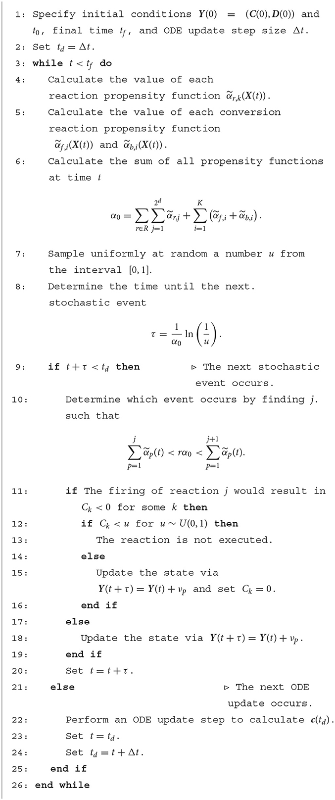
Algorithm 1. The regime-conversion method

3. Results

In this section we demonstrate the accuracy of the RCM for three example problems of increasing complexity. We choose to use the classical fourth-order Runge Kutta method [19, p. 352] for solving the systems of ODEs, and the GDM for simulating stochastic trajectories. We make special note that the validity of our coupling is independent of the chosen numerical method for simulating the system of ODEs. Nevertheless, the accuracy of the method as a whole will naturally depend to a large extent on the accuracy of the underlying numerical techniques; a phenomenon that we explore in Test Case 3.2. To measure the error in a simulation run, we define the relative error between the SSA and the RCM by

$\begin{array}{l}{\epsilon }_{k,\text{RCM}}(t)\stackrel{\text{def}}{=}\frac{f_{k,\text{RCM}}(t)-f_{k,\text{SSA}}(t)}{f_{k,\text{SSA}}(t)},\end{array}$

where f_k,SSA is the computed density of the k^th species at time t as approximated by the SSA (resp. by the RCM). Likewise, we define the relative error between the system of ODEs and the SSA by

$\begin{array}{l}{\epsilon }_{k,\text{ODE}}\stackrel{\text{def}}{=}\frac{f_{k,\text{ODE}}(t)-f_{k,\text{SSA}}(t)}{f_{k,\text{SSA}}(t)},\end{array}$

where f_k,ODE is the computed density of the k^th species at time t according to the system of ODEs as simulated by the numerical method.

3.1. Test case 1—Alternating exponential growth

Our first test case aims to demonstrate the accuracy of the method in the case of network with a single species, where continuous mass is degraded by a first-order degradation reaction to induce a continuous-to-discrete regime conversion, and discrete mass is produced by a zeroth-order production reaction to induce a discrete-to-continuous regime conversion. We thus consider the following simple reaction network $\mathcal{N}$ consisting of a single species X and two reactions,

$\begin{array}{l}\varnothing \underset{{\lambda }_2}{\overset{{\lambda }_1}{\rightleftharpoons }}X,\end{array}$

where the rates are of the form

$\begin{array}{l}{\lambda }_i(t)=\{\begin{array}{ll}{k}_i\hfill & t\in I_i,\hfill \\ 0\hfill & \text{otherwise,}\hfill \end{array}\end{array}$

where k_i > 0 and I_i is some finite, non-empty union of time intervals. In our specific example, we choose these intervals such that the degradation reaction is “on” precisely when the production reaction is “off”, and vice-versa. This network has stoichiometry matrix

$\begin{array}{l}\text{S}=\left[\begin{array}{cc}1& -1\end{array}\right],\end{array}$

and propensity functions

$\begin{array}{l}\begin{array}{cc}{\alpha }_1={\lambda }_1,& {\alpha }_2={\lambda }_{2}x.\end{array}\end{array}$

From this, we form the corresponding M-ARN $\mathcal{M}$ with two species C and D. This network has stoichiometry matrix

$\begin{array}{l}M=\left[\begin{array}{rr}\hfill 1& \hfill 0\\ \hfill 0& \hfill -1\end{array}|M_1\right],\text{ recalling }{M}_1=\left[\begin{array}{cc}1& -1\\ -1& 1\end{array}\right],\end{array}$

and propensity functions

$\begin{array}{l}{\tilde{\alpha }}_{1,1}={\lambda }_1,{\tilde{\alpha }}_{2,1}={\lambda }_{2}d,\end{array}$

corresponding to the zeroth-order production and the first-order degradation of discrete mass, respectively. The first-order degradation of continuous mass is modeled via the ODE

$\begin{array}{l}\frac{\text{d}}{\text{d}t}\langle C\rangle =-{\lambda }_2\langle C\rangle .\end{array}$

We present the results of this test case in Figure 1 using the parameter values given in Table 1. This proof-of-concept example demonstrates the key behavior of the RCM—the conversion between discrete- and continuum-governed mass. As expected, when overall density falls below the threshold value we observe the conversion of continuum to discrete mass, and vice versa when density again becomes sufficiently high. We observe no evidence of bias in the RCM, with the fluctuations away from zero in Figure 1A not persisting between simulation runs.

FIGURE 1

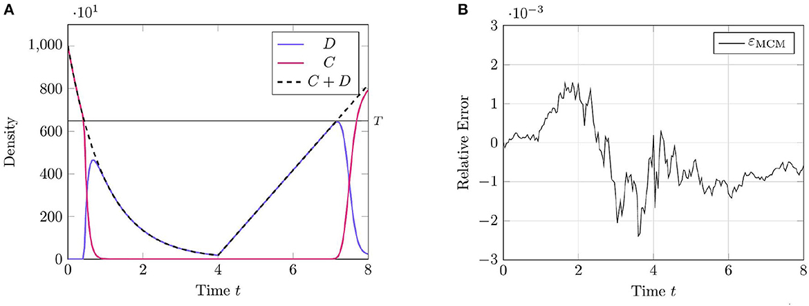
Figure 1. Results of Test Case 1 (Section 3.1) with parameters as specified in Table 1 with conversion threshold T = 650. Simulation results averaged over 10⁵ repeats. (A) Plot of the density of D + C as simulated by the RCM. (B) Relative error in D + C between the RCM and the SSA.

TABLE 1

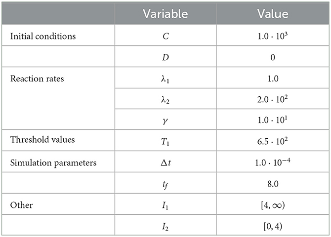
Table 1. Initial and parameter values for test problem 1.

3.2. Test case 2—Alternating logistic growth

Our second test case aims to demonstrate the accuracy of the method in the case of a network with a single species, this time where continuous mass is degraded by a second-order degradation reaction to induce a continuous-to-discrete regime conversion, and discrete mass is produced by a first-order production reaction to induce a discrete-to-continuous regime conversion. As in Test Case 1, we take $\mathcal{N}$ consisting of a single species X, this time with reactions

$\begin{array}{c}X\underset{{\lambda }_2}{\overset{{\lambda }_1}{\rightleftharpoons }}X+X,\end{array}$

where the rate λ₁ is constant over time and λ₂ is governed by

$\begin{array}{c}{\lambda }_2(t)=\{\begin{array}{ll}{k}_2\hfill & t\in I,\hfill \\ 0\hfill & \text{otherwise,}\hfill \end{array}\end{array}$

where k₂ > 0 and I is some finite, non-empty union of time intervals. Again, we select these intervals such that the production reaction is “on” precisely when the degradation reaction is “off”, and vice-versa. This network has stoichiometry matrix

$\begin{array}{c}\text{S}=\left[\begin{array}{cc}1& -1\end{array}\right],\end{array}$

this time with propensity functions

$\begin{array}{c}{\alpha }_1={\lambda }_{1}x,{\alpha }_2={\lambda }_{2}x(x-1).\end{array}$

Following extension, we obtain an ARN $\mathcal{M}$ with two species C and D. This network has stoichiometry matrix

$\begin{array}{c}M=\left[\begin{array}{rrrr}\hfill 1& \hfill 0& \hfill -1& \hfill 0\\ \hfill 0& \hfill -1& \hfill 0& \hfill -1\end{array}|M_1\right],\end{array}$

and propensity functions

$\begin{array}{c}\begin{array}{ccc}{\tilde{\alpha }}_{1,1}={\lambda }_{1}d,& {\tilde{\alpha }}_{2,1}={\lambda }_{2}d(d-1),& {\tilde{\alpha }}_{2,2}={\tilde{\alpha }}_{2,3}={\lambda }_{2}dc,\end{array}\end{array}$

representing the production of a discrete molecule from a discrete molecule, the degradation of a discrete molecule by a discrete molecule, the degradation of a continuous molecule by a discrete molecule, and the degradation of a discrete molecule by a continuous molecule, respectively. We form the equation governing the second-order degradation of continuous mass by continuous mass and the production of continuous mass from continuous mass using the Poisson closure; this equation is given by the ODE

$\begin{array}{c}\frac{\text{d}}{\text{d}t}\langle C\rangle ={\lambda }_1\langle C\rangle -{\lambda }_2{\langle C\rangle }^2.\end{array}$

We present the results of this test case in Figure 2 using the parameter values given in Table 2. The results of this test case demonstrate a particular limitation of the RCM; namely, that the error in the RCM is, in some sense, “tethered” to the error in the solution to the system of ODEs in the associated ARN. We see this most clearly at the parameter transition point t = 20, when the second-order reaction degradation activates.

FIGURE 2

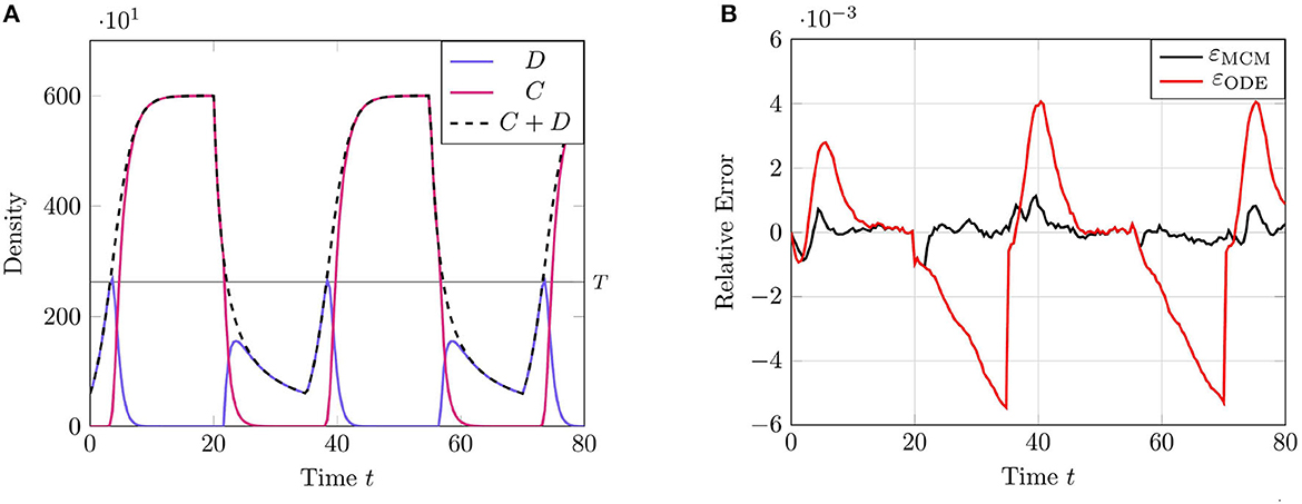
Figure 2. Results of Test Case 2 (Section 3.2) with parameters as specified in Table 2 with conversion threshold T = 300. Simulation results averaged over 10⁵ repeats. (A) Plot of the density of D + C as simulated by the RCM. (B) Relative error in D + C between the RCM and the SSA and between the system of ODEs and the SSA.

TABLE 2

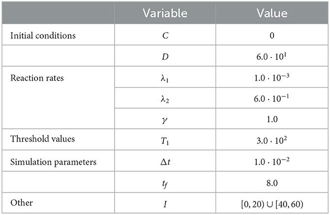
Table 2. Initial and parameter values for test problem 2.

3.3. Test case 3—Chemical signaling

For our third test case, consider a CRN, $\mathcal{N}$, consisting of three chemical species X₁, X₃, and X₂, which we refer to as the signal, intermediate, and product species respectively, within a reactor vessel of unit volume. The product X₂ is produced via the intermediate X₃ and is degraded via a first-order sink reaction. The intermediate is produced via a zeroth-order source reaction.

$\begin{array}{c}\varnothing {\displaystyle \underset{}{\overset{{\lambda }_1}{\to }}}{X}_3{\displaystyle \underset{}{\overset{{\lambda }_2}{\to }}}{X}_2{\displaystyle \underset{}{\overset{{\lambda }_3}{\to }}}\varnothing .\end{array}$

The signal species X₁ is coupled indirectly with X₂ via the following reaction,

$\begin{array}{c}{X}_1+X_3{\displaystyle \underset{}{\overset{{\lambda }_4}{\to }}}{X}_1,\end{array}$

in which the signal degrades the intermediate X₃. Finally, the signal species itself is produced and degraded according to the same reaction system we used in Test Case 1,

$\begin{array}{c}\varnothing \underset{{\lambda }_6}{\overset{{\lambda }_5}{\rightleftharpoons }}{X}_1.\end{array}$

This CRN, $\mathcal{N}$, has stoichiometry matrix

$\begin{array}{c}\mathcal{S}=\left[\begin{array}{cccccc}0& 0& 0& 0& 1& -1\\ 0& 1& -1& 0& 0& 0\\ 1& -1& 0& -1& 0& 0\end{array}\right],\end{array}$

with propensity functions given by

$\begin{array}{l}\begin{array}{ccc}{\alpha }_1={\lambda }_1,\hfill & {\alpha }_2={\lambda }_2{x}_3,& {\alpha }_3={\lambda }_3{x}_2,\\ {\alpha }_4={\lambda }_4{x}_1{x}_3,& {\alpha }_5={\lambda }_5,& {\alpha }_6={\lambda }_6{x}_1.\end{array}\end{array}$

Under the mean-field closure, the means of X₁, X₂, and X₃ are governed by the following system of ODEs

$\begin{array}{ll}\begin{array}{c}\frac{\text{d}\langle X_1\rangle }{\text{d}t}={\lambda }_5-{\lambda }_6\langle X_1\rangle ,\hfill \\ \frac{\text{d}\langle X_2\rangle }{\text{d}t}={\lambda }_2\langle X_3\rangle -{\lambda }_3\langle X_2\rangle ,\hfill \\ \frac{\text{d}\langle X_3\rangle }{\text{d}t}={\lambda }_1-{\lambda }_2\langle X_3\rangle -{\lambda }_4\langle X_1\rangle \langle X_3\rangle .\end{array}\hfill & (20)\end{array}$

As demonstrated in Paulsson et al. [20], the steady-state behavior of $\mathcal{N}$ is determined to a substantial degree by the stochastic fluctuations of X₃. This system, therefore, benefits greatly from a hybrid modeling approach, where the low-copy-number X₁ and X₃ can be modeled discretely. From the CRN $\mathcal{N}$ we form the M-ARN $\mathcal{M}$, which has stoichiometry matrix

$\begin{array}{c}{M}_R=\left[\begin{array}{cccccccc}0& 0& 0& 0& 0& 0& 0& 0\\ 0& 0& 0& 0& 0& 0& 0& 0\\ 0& 0& 0& 0& -1& 0& 0& 0\\ 0& 0& 0& 0& 0& 0& 1& -1\\ 0& 1& -1& 0& 0& 0& 0& 0\\ 1& -1& 0& -1& 0& -1& 0& 0\end{array}|M_3\right],\end{array}$

where M₃ is defined in equation (19); reaction propensities

$\begin{array}{l}\begin{array}{ccc}{\tilde{\alpha }}_{1,1}={\lambda }_1,\hfill & {\tilde{\alpha }}_{2,1}={\lambda }_2{d}_3,& {\tilde{\alpha }}_{3,1}={\lambda }_3{d}_2,\\ {\tilde{\alpha }}_{4,1}={\lambda }_4{d}_1{d}_3,& {\tilde{\alpha }}_{4,2}={\lambda }_4{d}_1{c}_3,& {\tilde{\alpha }}_{4,3}={\lambda }_4{c}_1{d}_3,\\ {\tilde{\alpha }}_{5,1}={\lambda }_5,\hfill & {\tilde{\alpha }}_{6,1}={\lambda }_6{d}_1,\end{array}\hfill \end{array}$

and; the following system of ODEs,

$\begin{array}{l}\begin{array}{c}\frac{\text{d}\langle C_1\rangle }{\text{d}t}=-{\lambda }_6\langle C_1\rangle ,\hfill \\ \frac{\text{d}\langle C_2\rangle }{\text{d}t}={\lambda }_2\langle C_3\rangle -{\lambda }_3\langle C_2\rangle .\hfill \\ \frac{\text{d}\langle C_3\rangle }{\text{d}t}=-{\lambda }_2\langle C_3\rangle -{\lambda }_4\langle C_1\rangle \langle C_3\rangle .\end{array}\hfill \end{array}$

To demonstrate the utility of the RCM in this case, we compare the mean densities of $\mathcal{N}$ as approximated by both the Gillespie SSA and by the mean-field equation (20) with the mean density of $\mathcal{M}$ as approximated by the RCM. For this problem, we wish to simulate the species X₁ and X₃ purely via the discrete regime and the product species X₂ will be permitted to switch regimes dependent on density. The model parameters used for our test case are listed in Table 3. We present the results of this test case in Figure 3. Notice that the density of D₂ appears to decrease before reaching the threshold value. This is to be expected since, as the system is governed wholly by the discrete regime until the threshold is reached, a non-zero number of simulation trajectories reach threshold before the mean trajectory. This manifests as the mean trajectory beginning regime transition before the threshold is actually reached.

TABLE 3

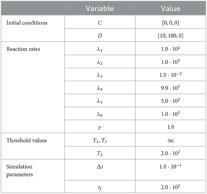
Table 3. Initial and parameter values for test problem 3.

FIGURE 3

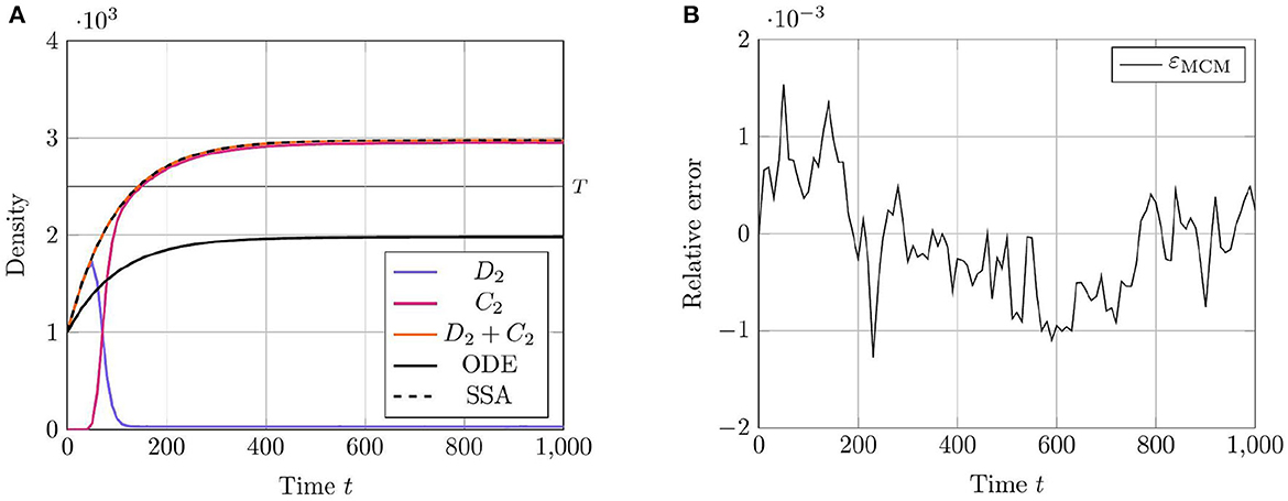
Figure 3. Results of Test Case 3 (Section 3.3) with parameter values given in Table 2. (A) Plot of the density of C₂ + D₂ as simulated by the RCM, SSA, and ODEs. Note that the density as determined by the SSA is indistinguishable at this scale from the density determined by the RCM—as such the trajectory of the RCM obscures that of the SSA in the plot. (B) Relative error in C₂ + D₂ between the RCM and the SSA. Simulation results averaged over 1.6 · 10⁴ repeats.

Evidently, the RCM substantially outperforms the mean-field ODEs at approximating the true trajectory of this reaction network. The reason for this is that the RCM guarantees the simulation of the X₃ species exclusively via the discrete regime by setting the relevant regime conversion threshold values to infinity. As such, the method retains information of the stochastic fluctuations in X₃ where the system of mean-field ODEs does not. We further note the lack of bias in the error of the RCM.

3.4. Test case 4—Michaelis-Menten enzyme kinetics

Here we apply the RCM to the well-studied Michaelis-Menten model of enzyme kinetics [21, 22]. We consider a slight generalization of the classical model wherein the substrate species is continuously supplied to the system. The model can be represented as a CRN with the following reactions:

$\begin{array}{cc}\varnothing \stackrel{{\lambda }_1}{\to }S,E+S\underset{{\lambda }_4}{\overset{{\lambda }_3}{\rightleftharpoons }}M\stackrel{{\lambda }_4}{\to }E+P.& (21)\end{array}$

This network models the conversion of a substrate species S into a product species P via catalysis with some enzyme E. This conversion occurs when a member of the substrate species binds with the enzyme to form an intermediate enzyme-substrate complex M. The complex M can then unbind either into its original constituents E + S or into a new product P, freeing the enzyme E to bind with further substrate. Note that, since E acts only as a catalyst in the above network, the quantity E_T = E + M is conserved over time.

For the purposes of our demonstration, tracking the growth in copy number of the species P is unimportant. Thus, we henceforth neglect to include this species in the network, though we retain the reaction channel to leave the dynamics of the remaining species unchanged. Taking the mean-field closure of the master equation formed from the system of reactions (21), we obtain the following system of ODEs:

$\begin{array}{c}\begin{array}{c}\frac{\text{d}\langle S\rangle }{\text{d}t}={\lambda }_1-{\lambda }_2\langle E\rangle \langle S\rangle +{\lambda }_3\langle M\rangle ,\hfill \\ \frac{\text{d}\langle E\rangle }{\text{d}t}=-{\lambda }_2\langle E\rangle \langle S\rangle +({\lambda }_3+{\lambda }_4)\langle M\rangle ,\hfill \\ \frac{\text{d}\langle M\rangle }{\text{d}t}={\lambda }_2\langle E\rangle \langle S\rangle -({\lambda }_3+{\lambda }_4)\langle M\rangle ,\hfill \end{array}\end{array}$

which can be shown to have a steady-state solution given by

$\begin{array}{c}\langle S\rangle =\frac{{\lambda }_1({\lambda }_3+{\lambda }_4)}{{\lambda }_2({\lambda }_4{E}_T-{\lambda }_1),}\\ \langle M\rangle =E_T-\langle E\rangle =\frac{{\lambda }_1}{{\lambda }_4}.\end{array}$

We now form the M-ARN for system (21), which has stoichiometry matrix

$\begin{array}{l}\begin{array}{c}{M}_R=[\begin{array}{cccccc}0& 0& 0& -1& 0& 0\\ 0& 0& -1& 0& 0& 0\\ 0& 0& 0& 0& 0& 0\\ 1& -1& -1& 0& 1& 0\\ 0& -1& 0& -1& 1& 1\\ 0& 1& 1& 1& -1& -1\end{array}|M_3],\end{array}\end{array}$

reaction propensities

$\begin{array}{c}\begin{array}{ccc}{\tilde{\alpha }}_{1,1}={\lambda }_1,\hfill & {\tilde{\alpha }}_{2,1}={\lambda }_2{d}_E{d}_S,& {\tilde{\alpha }}_{2,2}={\lambda }_2{c}_E{d}_S,\\ {\tilde{\alpha }}_{2,3}={\lambda }_2{d}_E{c}_S,& {\tilde{\alpha }}_{3,1}={\lambda }_3{d}_M,& {\tilde{\alpha }}_{4,1}={\lambda }_4{d}_M,\end{array}\end{array}$

and the following system of ODEs,

$\begin{array}{c}\begin{array}{c}\frac{\text{d}\langle C_S\rangle }{\text{d}t}=-{\lambda }_2\langle C_E\rangle \langle C_S\rangle +{\lambda }_3\langle C_M\rangle ,\hfill \\ \frac{\text{d}\langle C_E\rangle }{\text{d}t}=-{\lambda }_2\langle C_E\rangle \langle C_S\rangle +({\lambda }_3+{\lambda }_4)\langle C_M\rangle ,\hfill \\ \frac{\text{d}\langle C_M\rangle }{\text{d}t}={\lambda }_2\langle C_E\rangle \langle C_S\rangle -({\lambda }_3+{\lambda }_4)\langle C_M\rangle .\hfill \end{array}\end{array}$

As in prior test cases, we again evaluate the accuracy of the RCM against the Gillespie SSA. For this system, we select parameters such that all species except for the enzyme species E are simulated using the continuous regime in order to evaluate how well the RCM performs at estimating both the mean and the variance of E at steady state. We present the results for the mean estimate in Figure 4. The model parameters used for this test case are listed in Table 4. This case highlights a key feature of the RCM. Notice that, despite E having a threshold of ∞ (and therefore suggesting that all mass should be governed by the discrete regime), a small proportion of the mass is nevertheless represented by the continuous regime at steady state. This proportion can be tweaked to different values depending on the specific enzymatic reaction being modeled by increasing or decreasing the regime transition rates γ_f,E and γ_b,E. This non-zero mass C_E, as well as the fact that all other species are governed primarily by the continuous regime, manifests as a slight positive bias in the RCM vs. the SSA (Figure 4B). A parameter sweep demonstrates that this bias is reduced by decreasing the step size used in the numerical method; however, this naturally comes at greater computational cost.

FIGURE 4

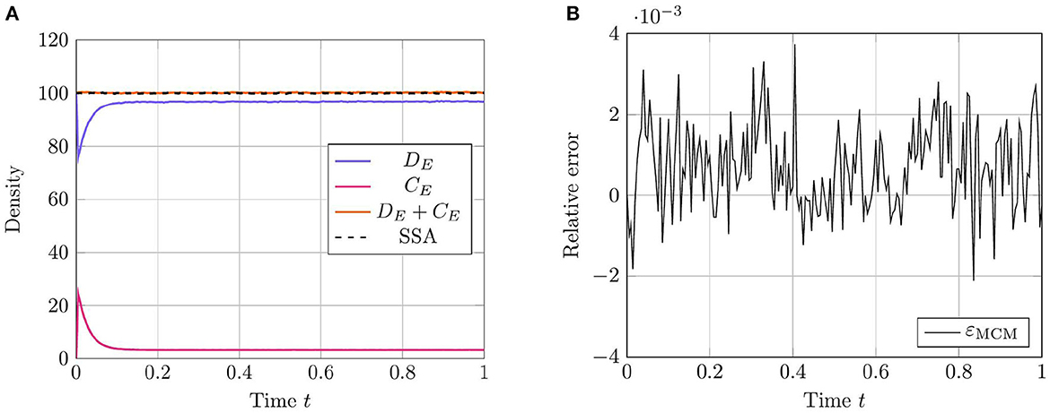
Figure 4. Results of Test Case 4 (Section 3.4) with parameter values given in Table 3. Simulation results averaged over 1 · 10⁵ repeats. (A) Plot of the density of D_E + C_E as simulated by the RCM. Shown is the amount of mass D_E in the discrete regime and the amount of mass C_E in the continuous regime, alongside the total mass D_E + C_E. Results from the SSA over the same time period are overlaid. (B) Relative error in the density of D_E + C_E as predicted by the RCM and vs. the SSA over time.

TABLE 4

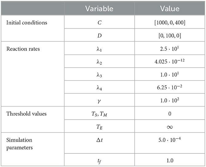
Table 4. Initial and parameter values for test problem 4.

Figure 5 compares the steady-state distribution of the mass of E as estimated by the RCM vs. the SSA. In both cases, we consider the system to have reached steady state by t = 5, and sample the distribution of E at this time. Here, we observe that while the overall shape of the distribution is largely preserved, the variance predicted by the RCM is slightly lower than that predicted by the SSA, as evidenced by the thinner tails of the distribution. Unlike the bias in the mean, this damping of the variance is not dependent on the step size used. This discrepancy in the variance is perhaps unsurprising, given that a proportion of E is governed by the (approximate and deterministic) continuous regime.

FIGURE 5

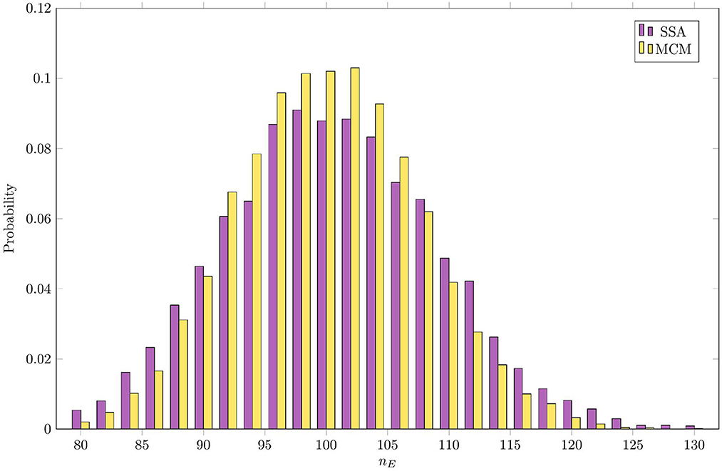
Figure 5. Steady-state distribution of the amount of mass in species E as estimated by the RCM vs. the SSA.

4. Discussion

In this work we introduced a novel hybrid method for simulating well-mixed chemical reaction networks. This method couples a system of ODEs with a Markov process representation of a chemical reaction network by constructing a so-called augmented reaction network that combines both representations. The continuous and discrete components of the augmented network can be simulated simultaneously using different techniques to maximize computational efficiency and minimize the loss of accuracy resultant from taking continuum approximations. We demonstrated the accuracy of the method in three separate test problems of increasing complexity, evidencing in the final test case a substantial improvement in accuracy using our method vs. the standard continuum approximation technique.

While our method demonstrates substantially better accuracy vs. the continuum-only models in the test cases we present, its advantage vs. a traditional SSA is, in general, dependent on network structure. Specifically, in systems where the majority of computation time (when simulated via a SSA) is spent on the simulation of low copy-number species interacting with high copy-number species via bimolecular reaction channels, there is little computational benefit to our approach. The reason for this is that such reactions are (assuming each species is below and above the transition thresholds, respectively) necessarily simulated using the SSA, and therefore may impart no computational benefit in the RCM vs. the SSA alone. In cases where both reactant species in a bimolecular reaction are of sufficiently high concentration to be above their respective transition thresholds, it may be the case that the RCM yields similar accuracy to that of a continuum-based approach. Nevertheless, in neither case is there reason to expect a priori that use of the RCM is necessarily disadvantageous. With these caveats in mind, there are clear instances where the RCM may be suitable to use over traditional methods. In loosely-coupled networks where the majority of interactions are of first-order (networks of this type frequently arise when modeling cellular populations [23–26]), the RCM demonstrates a clear computational advantage.

Another limitation of the RCM is that it may estimate moments of order two and above with some inaccuracy. This is a limitation shared by several other hybrid methods [11, 12]. Indeed, we see that by simulating a significant proportion of the dynamics of a system via the continuous method (as seen in Test Case 3.4, one induces a damping effect on the variance in species numbers. Nevertheless, the results demonstrate that the RCM allows for partial recovery of the distributions of constituent species. A possible solution to this problem would be to replace the system of deterministic, mean-field ODEs governing the continuous regime with appropriate stochastic differential equations. This approach has been used to solve the variance damping problem in spatial hybrid methods [27]. Additional work is required to conduct a full examination of the evolution of higher-order moments in the RCM and to quantify how such evolution is related to model parameters.

Our method differs from similar hybrid methods [11–13] in two crucial ways. First, our method allows for mass to transition dynamically between regimes. While it is possible to set thresholds (by setting threshold values to 0 or ∞) and transition rates (by setting transition rates to particularly small or particularly large values) such that mass is preferentially represented by one of the two regimes, the intended use case of the RCM is for systems where there is significant variability in the copy number of one of more species over the course of a simulation run. Second, in many cases, species simulated by the RCM have both a discrete and a continuous component. This allows for the partial recovery of these species' distributions, which would not be possible with a continuum-only approximation of the first moments of a network.

There are several ways in which the RCM might be extended to accommodate a wider variety of problems and to increase its computational efficiency. The first and most obvious direction is to extend its dimensionality; for example, to a spatial setting. The RCM, being an effective simulation technique for well-mixed reaction networks, might be extended to a spatial reaction-diffusion setting in several ways. Under a mesoscopic modeling regime [8], where individual system components are collected into well-mixed spatial “bins” of fixed size, the RCM could be used to simulate reactions by treating individuals in each bin as distinct species that do not interact with neighboring bins. In this framework, diffusive jumps between bins are simply reactions that convert individuals in one “bin species” to another. A spatial model consisting of binned particles and ordinary differential equations associated with each bin is thereby easily treated via the RCM. Nevertheless, this representation of a reaction-diffusion process is limited - for spatial domains with many bins, simulating large systems of (potentially) non-linear ODEs may be prohibitively expensive. A more sensible choice would be to represent the continuous approximation as a system of partial differential equations on an explicitly spatial domain; indeed, contemporary spatially-extended hybrid methods that couple continuous and mesoscopic regimes generally use this representation [8]. In this case, the matter of coupling the stochastic and diffusive reactions in each bin is not so straightforward, requiring numerical integration of the partial differential equation over relevant spatial regions. Extending the RCM in this manner to a spatially-extended mesoscopic-to-continuous hybrid method will form the basis of an upcoming investigation.

The RCM may also be extended to incorporate additional dimensionality along non-spatial lines. An important class of demographic and biological models are those with size- or age-structure, or a combination thereof. These model systems of interacting individuals (either eukaryotic or prokaryotic cells) undergoing some variant of the classical cell-cycle [28], and for which an individual's size (or age) is an important contributor to overall population dynamics. These systems are often modeled as either discrete-state stochastic processes [26, 29–31] or as continuous partial differential equations via the McKendrick-von Foerster equation [32, 33]. Despite their ubiquity, to the best of the authors' knowledge there exist no hybrid simulation techniques that can accommodate, without modification, size- or age-structure. Depending on the specific functional form of any size- or age-mediated reactions, a method of “spatial” numerical integration over intervals of age or size similar to that proposed for spatial extension may prove fruitful for coupling these two modeling regimes.

An important area of research in numerical methods in general is the development of so-called “adaptive” methods. These are methods for which certain numerical parameters can be changed mid-way through a simulation run to adapt to situations that might otherwise prove numerically challenging or computationally infeasible. The prototypical example of this is in adaptive time-stepping methods for solving systems of ordinary differential equations, wherein the usual fixed time step of a numerical solver is replaced with a variable time step that is recalculated at each update step to ensure stability even when the derivatives of the system undergo large variations [34]. As noted in our description of the RCM, one could apply such an adaptive time-stepping method for computing approximations to the continuum regime description without needing to modify the algorithm. Nevertheless, it is not difficult to conceive of a more specialized form of time-stepping that would take into consideration more than just the mass in the continuous regime and instead consider both the discrete mass and the calculated propensity functions at the time of an update step. For example, large numbers of individuals either entering or leaving the continuous regime may, by affecting the gradient of the continuum approximation, inject undesirable numerical instabilities into the RCM in extreme cases—something that traditional adaptive time-stepping methods are not designed to handle. Adaptivity in terms of time-stepping is not the only potential improvement, however. Presently, the RCM requires that the threshold values for the regime conversion reactions are set and fixed a priori. One can envisage modifications to the RCM where the conversion thresholds vary in response to changes in density, computational cost, rates of density change, and the stochasticity present in the system at any given time.

Finally, the method may be extended to incorporate reactions of arbitrary molecular order. While any reactions of molecular order of at least three can be decomposed into sequences of reactions of molecular order of at most two, these decompositions can be difficult to compute in practice. We conjecture that the same techniques used to demonstrate equivalence between the CRN and its associated ARN apply to higher-order reactions; however, proving this in generality is likely to be cumbersome. Further, one needs 2^d ODEs to satisfy the coupling requirements C1, C2 for a reaction of order d which, while not necessarily impacting computation time, may quickly become impractical to implement for large networks.

To summarize, our method provides a novel and computationally efficient technique for simulating well-mixed chemical reactions networks using a hybrid discrete/continuous methodology. Unlike similar existing methods, ours does not depend on the system of interest possessing certain properties; i.e., a particular decomposability of reactions or species into “fast” and “slow” categories. Further, it represents a promising coupling mechanism between the mesoscopic and macroscopic regimes that may permit for the development of new spatially-extended hybrid techniques that have a particular intrinsic adaptivity; namely, the ability to simulate spatial density distributions with significant and dynamic heterogeneity.

Data availability statement

The raw data supporting the conclusions of this article will be made available by the authors, without undue reservation.

Author contributions

AH performed preliminary investigations. JK performed the numerical and mathematical analysis and took lead in writing and preparing the manuscript. CY and CG provided feedback and suggestions during the analysis. All authors contributed to the design and conception of the method, and read and approved the submitted version.

Funding

JK is supported by a scholarship from the EPSRC Centre for Doctoral Training in Statistical Applied Mathematics at Bath (SAMBa), under the project EP/L015684/1.

Conflict of interest

The authors declare that the research was conducted in the absence of any commercial or financial relationships that could be construed as a potential conflict of interest.

Publisher's note

All claims expressed in this article are solely those of the authors and do not necessarily represent those of their affiliated organizations, or those of the publisher, the editors and the reviewers. Any product that may be evaluated in this article, or claim that may be made by its manufacturer, is not guaranteed or endorsed by the publisher.

References

1. Wilkinson DJ. Stochastic Modelling for Systems Biology. New York: CRC Press. (2020).

Google Scholar

2. Gillespie DT. Exact stochastic simulation of coupled chemical reactions. J Phys Chem. (1977) 81:2340–61. doi: 10.1021/j100540a008

PubMed Abstract | CrossRef Full Text | Google Scholar

3. Gibson MA, Bruck J. Efficient exact stochastic simulation of chemical systems with many species and many channels. J Phys Chem A. (2000) 104:1876–89. doi: 10.1021/jp993732q

CrossRef Full Text | Google Scholar

4. Cao Y, Li H, Petzold L. Efficient formulation of the stochastic simulation algorithm for chemically reacting systems. J Chem Phys. (2004) 121:4059–67. doi: 10.1063/1.1778376

PubMed Abstract | CrossRef Full Text | Google Scholar

5. Anderson DF. A Modified next reaction method for simulating chemical systems with time dependent propensities and delays. J Chem Phys. (2007) 127:214107. doi: 10.1063/1.2799998

PubMed Abstract | CrossRef Full Text | Google Scholar

6. Gillespie DT. A rigorous derivation of the chemical master equation. Physica A. (1992) 188:404–25. doi: 10.1016/0378-4371(92)90283-V

CrossRef Full Text | Google Scholar

7. Schnoerr D, Sanguinetti G, Grima R. Comparison of different moment-closure approximations for stochastic chemical kinetics. J Chem Phys. (2015) 143:185101. doi: 10.1063/1.4934990

PubMed Abstract | CrossRef Full Text | Google Scholar

8. Smith CA, Yates CA. Spatially extended hybrid methods: a review. J R Soc Interface. (2018) 15:20170931. doi: 10.1098/rsif.2017.0931

PubMed Abstract | CrossRef Full Text | Google Scholar

9. Cao Y, Gillespie DT, Petzold LR. The slow-scale stochastic simulation algorithm. J Chem Phys. (2005) 122:014116. doi: 10.1063/1.1824902

PubMed Abstract | CrossRef Full Text | Google Scholar

10. Cotter SL, Zygalakis KC, Kevrekidis IG, Erban R. A constrained approach to multiscale stochastic simulation of chemically reacting systems. J Chem Phys. (2011) 135:094102. doi: 10.1063/1.3624333

PubMed Abstract | CrossRef Full Text | Google Scholar

11. Hellander A, Lötstedt P. Hybrid method for the chemical master equation. J Comp Phys. (2007) 227:100–22. doi: 10.1016/j.jcp.2007.07.020

PubMed Abstract | CrossRef Full Text | Google Scholar

12. Smith S, Cianci C, Grima R. Model reduction for stochastic chemical systems with abundant species. J Chem Phys. (2015) 143:214105. doi: 10.1063/1.4936394

PubMed Abstract | CrossRef Full Text | Google Scholar

13. Jahnke T. On reduced models for the chemical master equation. Multiscale Model Simul. (2011) 9:1646–76. doi: 10.1137/110821500

CrossRef Full Text | Google Scholar

14. Van Kampen NG. Stochastic Processes in Physics and Chemistry. 3rd ed London: Elsevier. (2007). doi: 10.1016/B978-044452965-7/50006-4

CrossRef Full Text | Google Scholar

15. Barrat A, Barthélemy M, Vespignani A. Dynamical Processes on Complex Networks. 1st ed. Cambridge: Cambridge University Press (2008). doi: 10.1017/CBO9780511791383

CrossRef Full Text | Google Scholar

16. Nåsell I. An extension of the moment closure method. Theor Popul Biol. (2003) 64:233–239. doi: 10.1016/S0040-5809(03)00074-1

PubMed Abstract | CrossRef Full Text | Google Scholar

17. Laidler KJ. Reaction Kinetics. 1st ed Pergamon: Elsevier. (1963). doi: 10.1016/B978-1-4831-9738-8.50005-4

CrossRef Full Text | Google Scholar

18. Aris R, Gray P, Scott SK. Modelling cubic autocatalysis by successive bimolecular steps. Chem Eng Sci. (1988) 43:207–11. doi: 10.1016/0009-2509(88)85032-2

CrossRef Full Text | Google Scholar

19. Suli E, Mayers DF. An Introduction to Numerical Analysis. Cambridge: Cambridge University Press. (2003).

Google Scholar

20. Paulsson J, Berg OG, Ehrenberg M. Stochastic Focusing: Fluctuation-Enhanced Sensitivity of Intracellular Regulation. PNAS. (2000) 97:7148–53. doi: 10.1073/pnas.110057697

PubMed Abstract | CrossRef Full Text | Google Scholar

21. Michaelis L, Menten ML. Die Kinetik Der invertinwirkung. Biochem Z. (1913) 49:352.

Google Scholar

22. Murray JD. Reaction Kinetics. In: Murray JD, editor. Mathematical Biology. New York, NY: Springer New York (1993). p. 175–217. doi: 10.1007/978-0-387-22437-4_6

CrossRef Full Text | Google Scholar

23. Simpson MJ, Towne C, McElwain DS, Upton Z. Migration of breast cancer cells: understanding the roles of volume exclusion and cell-to-cell adhesion. Phys Rev E. (2010) 82:041901. doi: 10.1103/PhysRevE.82.041901

PubMed Abstract | CrossRef Full Text | Google Scholar

24. Simpson MJ, Landman KA, Hughes BD. Cell invasion with proliferation mechanisms motivated by time-lapse data. Physica A. (2010) 389:3779–90. doi: 10.1016/j.physa.2010.05.020

CrossRef Full Text | Google Scholar

25. Yates CA, Ford MJ, Mort RL. A multi-stage representation of cell proliferation as a Markov process. Bull Math Biol. (2017) 79:2905–28. doi: 10.1007/s11538-017-0356-4

PubMed Abstract | CrossRef Full Text | Google Scholar

26. Kynaston JC, Guiver C, Yates CA. Equivalence framework for an age-structured multistage representation of the cell cycle. Physical Review E. (2022) 105:064411. doi: 10.1103/PhysRevE.105.064411

PubMed Abstract | CrossRef Full Text | Google Scholar

27. Alexander FJ, Garcia AL, Tartakovsky DM. Algorithm refinement for stochastic partial differential equations: I. Linear Diffusion. J Comp Phys. (2002) 182:47–66. doi: 10.1006/jcph.2002.7149

CrossRef Full Text | Google Scholar

28. Schafer KA. The cell cycle: a review. Vet Pathol. (1998) 35:461–78. doi: 10.1177/030098589803500601

PubMed Abstract | CrossRef Full Text | Google Scholar

29. Stukalin EB, Aifuwa I, Kim JS, Wirtz D, Sun SX. Age-dependent stochastic models for understanding population fluctuations in continuously cultured cells. J R Soc Interface. (2013) 10:325. doi: 10.1098/rsif.2013.0325

PubMed Abstract | CrossRef Full Text | Google Scholar

30. Greenman CD, Chou T. A kinetic theory for age-structured stochastic birth-death processes. Phys Rev E. (2016) 93:012112. doi: 10.1103/PhysRevE.93.012112

PubMed Abstract | CrossRef Full Text | Google Scholar

31. Chou T, Greenman CD. A hierarchical kinetic theory of birth, death and fission in age-structured interacting populations. J Stat Phys. (2016) 164:49–76. doi: 10.1007/s10955-016-1524-x

PubMed Abstract | CrossRef Full Text | Google Scholar

32. Trucco E. Mathematical models for cellular systems. The von Foerster equation Part I B. Math Biophys. (1965) 27:285–304. doi: 10.1007/BF02478406

PubMed Abstract | CrossRef Full Text | Google Scholar

33. Rossini L, Contarini M, Speranza S. A Novel version of the von Foerster equation to describe poikilothermic organisms including physiological age and reproduction rate. Ric Mat. (2021) 70:489–503. doi: 10.1007/s11587-020-00489-6

CrossRef Full Text | Google Scholar

34. Hairer E, Norsett SP, Wanner G. Solving Ordinary Differential Equations I: Nonstiff Problems. New York: Springer. (1987). doi: 10.1007/978-3-662-12607-3

CrossRef Full Text | Google Scholar