Dynamic high-frequency dependence structure of Chinese agricultural commodity futures based on the semi-parametric copula

1. Introduction

The diminishing stocks of agricultural products in recent years have raised concerns about food security, particularly in the developing countries. This in turn has increased the volatility in agricultural commodity prices as evidence in the unprecedented price spikes during the world food crisis (2007–2008)¹ and sharp increases during the period from 2010 to 2011. Moreover, the complexity of agricultural commodity futures markets has increased significantly in recent years. It is known that there were sharp increases in dependence between international equity markets around the world during the global financial crisis (see e.g., [7–9]), more and more investors include commodity futures as a part of their diversified portfolios. Even though agricultural commodity futures seem to provide investors and portfolio managers with additional diversification benefits, if the agricultural commodity futures co-move closely as the underlying agricultural commodities do², the effectiveness of the diversification strategies and hedging potential among those agricultural commodity futures might be low and even disappear. Therefore, given their economic significance and growing importance in investment portfolios, it is vital to investigate the dependence structure between the agricultural commodity futures.

Previous studies mainly focus on the relationship between the spot and the futures prices for agricultural commodities [2] and the dependence between energy and agricultural commodities markets or between the stock and the agricultural commodities markets (e.g., [11–16]). The literature on the dependence between agricultural commodities is limited and most studies use various versions of multivariate GARCH models based on low-frequency data, such as daily or monthly data. Von Ledebur et al. [3] use a MGARCH model with daily price data to examine the volatility linkages between the agricultural commodities during the dramatic price changes in 2008, and find supporting evidence for dependence. Le Pen and Sevi [17] employ a factor model and a dynamic condition correlation (DCC) model with monthly price data to study the interrelationship among eight agricultural and none agricultural commodities and find weak evidence of dependence in price and volatility. Zhao and Goodwin [18] reveal important volatility linkages between the corn and soybean futures by using a threshold and BEKK model with weekly price data. Lahiani et al. [19] find strong evidence of dependence between the four major agricultural commodities including sugar, wheat, cotton, and corn by employing the VAR-GARCH model of Ling and McAleer [20] with daily price data. Beckmann and Czudaj [21] suggest the pairwise short-run volatility linkages between corn, wheat, and cotton futures by employing a bivariate GARCH-in-mean VAR models with daily price data. Using the standard full BEEK and DCC model with daily price data, Hernandez et al. [22] support the volatility linkages between corn, wheat and soybean across different futures markets in the United States, Europe, and Asia as well as an increase in their dependence in recent years. Gardebroek et al. [1] utilize both a full T-BEKK model and various T-DCC models with various data frequencies (daily, weekly, and monthly) to study the market interrelationships and volatility linkages among major agricultural commodities in the United States and find little evidence of dependence in levels but significant volatility linkage, particularly at weekly and monthly frequencies. There are some copula based models proposed in literatures to study dependence between commodities, such as the time-varying copula with a switching dependence [23], wavelet-based copula approach [24].

Chinese agricultural commodity futures market is selected for a few reasons. Agriculture is of special economic and political importance to China due to its large population. Further, the trading volume in Chinese agricultural commodity futures was about 292 trillion Yuan at the end of 2014, and ten out of the top 20 agricultural contracts by volume were traded on the Chinese exchanges according to the Futures Industry Association (FIA) statistics in the USA³. These figures show that Chinese agricultural commodity futures market has become the world's biggest market and has an increasing influence on the global pricing and the decisions on portfolio diversification (e.g., [25]). Finally, it should be noted that the futures trading in China is subject to some unique regulations such as the time-dependent margin rate for deposit, which may make Chinese futures market different from other developed markets. Therefore, it is also of special interest to study the dependence between Chinese agricultural commodity futures and their changing pattern over time.

To Consider the two properties of an agricultural commodity futures market, i.e., property of agricultural commodity due to the underlying asset, and property of finance due to the futures trading, we mainly aims to explore the dependence structure of futures during the world food crisis (2007–2008) and the global financial crisis (2008–2011). The 5-min and daily high frequency trading dataset covers the period from January 2006 to November 2014 are used. This sample period thus allows us to analyze the dynamics of dependence structure between different agricultural commodity futures during the two crisis periods.

This paper investigates the dynamic dependence structure between four Chinese agricultural commodity futures. The main contributions of this paper to reveal the typical characteristics of high frequency dependence structure of Chinese agricultural commodity futures, and to propose the semi-parametric copula-based multivariate model with high-frequency trading data. In contrast to the traditional GARCH approach, this approach has the additional benefit of allowing the investigation of tail and asymmetrical dependence. Further, the use of the high-frequency data not only allows us to observe the evolution of the latent conditional dependence, which is much less sensitive to structural breaks, but also allows us to investigate the intraday dependence patterns between each pair of agricultural commodity futures. To our best knowledge, the copula approach with high frequency data as employed in this paper has not been previously considered in the literature.

The remainder of the paper is organized as follows. Section 2 discusses the models. Section 3 presents the data and descriptive statistics. The empirical results are reported and analyzed in Section 4. The concluding remarks are given in Section 5.

2. Models

Due to the fact that the semi-parametric Copula-Based Multivariate Dynamic (SCBMD) model [26] allows for the conditional mean and conditional variance of the individual futures return series to be modeled, and the dependence of the scale-free residuals to be specified by a copula, we employ the high frequency data in each trading day to estimate this model and then obtain the daily copula dependence between the agricultural commodity futures, which is named the intraday dependence estimators in this paper, just as the daily realized correlation [27] is obtained from the high frequency data.

2.1. The semi-parametric copula model

2.1.1. The copula function

We utilize the copula function to investigate the dependence structure between the agricultural commodity futures in China as it provides the information on the average dependence and tail dependence between two agricultural commodity futures. Based on Sklar [28], we can break down the joint distribution of two continuous random variables X and Y, F_XY(x,y) into the marginal distribution functions F_X(x) and F_Y(y) that describe the individual behavior of each series. The copula function that fully captures the dependence structure between them is given by:

$\begin{array}{ll}F(x,y)=C(F_X(x),F_Y(y)),& (1)\end{array}$

where C(u, v), u = F_X(x) and v = F_Y(y) is the copula function that is solely relied on the ranges of F_X(x) and F_Y(y) if the margins are continuous. Thus, we can also represent the joint density of X and Y variables as:

$\begin{array}{ll}{f}_{XY}(x,y)=c(u,v)f_X(x)f_Y(y),& (2)\end{array}$

where f_X(x) and f_Y(y) are the marginal densities, and c(u, v) = ∂²C(u, v)/∂u∂v.

The copula function has several advantages for investigating the dependence between the agricultural commodity futures. First, by using the copula, we can model the marginal behavior of agricultural commodity futures prices and the dependence structures separately. Thus, the copula approach provides greater flexibility in modeling and estimating the margins and dependence than the parametric multivariate distributions. Second, the copula approach provides the information on both the degree and the structure of dependence, i.e., a more accurate measure of dependence than the traditional dependence measures given by the linear correlation, which only takes into account how agricultural commodity futures prices move together on average across marginal distributions with the assumption of multivariate normality. Third, as the copula is a multivariate distribution function with uniform (0,1) margins that associate the quantiles of the distributions instead of the original variables, the copula function is unaffected by the increasing and continuous transformations of agricultural commodity futures prices while the linear correlation is only invariant to linear transformations. This is important as dependence is the same for agricultural commodity futures prices as for the log returns of agricultural futures. Finally, the copula function allows us to investigate the tail dependence, which measures the probability that agricultural commodity futures go up or down together. The coefficient of upper (right) and lower (left) tail dependence can be described in terms of copula as:

$\begin{array}{l}{\tau }^U\mathrm{\text{=}}{\displaystyle \underset{u\to 1}{lim}}Pr[X\ge {\displaystyle F_X^{-1}}(u)|Y\ge F_Y^{-1}(u)]={\displaystyle \underset{u\to 1}{lim}}\frac{1-2u+C(u,u)}{1-u}\end{array}(3)$

$\begin{array}{l}{\tau }^L\mathrm{\text{=}}{\displaystyle \underset{u\to 0}{lim}}Pr[X\le {\displaystyle F_X^{-1}}(u)|Y\le F_Y^{-1}(u)]={\displaystyle \underset{u\to 0}{lim}}\frac{C(u,u)}{u}\end{array}(4)$

Where $F_X^{-1}$ and $F_Y^{-1}$ are the marginal quantile functions, τ^U and τ^L are always in [0,1]. When τ^U (τ^L) is 0, the two series are upper (lower) tail independent. Otherwise the series are tail dependent with higher values indicating more dependence in extreme events.

Thus, in order to investigate the dependence structure between the agricultural commodity futures through the copula approach, we need to model the marginal distribution and the joint distribution for each pair of agricultural commodity futures series.

2.1.2. The marginal distribution model

In order to capture the properties of intraday returns, such as conditional heteroskedasticity and leverage effects, we use the ARMA(p,q)–EGARCH(r,m) model as the marginal distribution model for asset i on trading day t:

$\begin{array}{ll}{r}_{i,t,j}=c_{i,t}+{\displaystyle \sum _{p_1=1}^p}{\varphi }_{p_1,i,t}{r}_{i,t,j-p_1}+{\epsilon }_{i,t,j}\text{+}{\displaystyle \sum _{q_1=1}^q}{\theta }_{q_1,i,t}{\epsilon }_{i,t,j-q_1},& (5)\end{array}$

$\begin{array}{ll}{\epsilon }_{i,t,j}={\sigma }_{i,t,j}{z}_{i,t,j},& (6)\end{array}$

$\begin{array}{l}log({\sigma }_{i,t,j}^2)={\omega }_{i,t}+{\displaystyle \sum _{r_1=1}^r}{\beta }_{r_1,i,t}log({\sigma }_{i,t,j-r_1}^2)+\\ {\displaystyle \sum _{m_1=1}^m}{\alpha }_{m_1,i,t}\left|\frac{{\epsilon }_{i,t,j-m_1}}{{\sigma }_{i,t,j-m_1}}\right|+{\displaystyle \sum _{m_1=1}^m}{\lambda }_{m_1,i,t}\frac{{\epsilon }_{i,t,j-m_1}}{{\sigma }_{i,t,j-m_1}}\end{array}(7)$

where I = 1, …K, j = 1, …, n, n is the number of intraday returns used in the desired sampled window. c_i,t, ϕ_p1,i,t, θ_q1,i,t, ω_i,t, β_r1,i,t, α_m1,i,t and λ_m1,i,t are different for each asset i, on each day t and are a function of n.

In order to reduce the risk of mis-specifying the marginal distributions of z_i,t,j, following Chen and Fan [26], we adopt the empirical marginal distributions for each day t to estimate F_i,t(z_i,t,j):

$\begin{array}{ll}{\widehat{F}}_{i,t}(x)=\frac{n}{n+1}{\displaystyle \sum _{j=1}^n}I({ẑ}_{i,t,j}\le x),-\infty <x<\infty & (8)\end{array}$

Where ẑ_i,t,j are the estimated standardized intraday residuals from Eq. (6). The numbers of lag p and q in Eq. (5) are selected for each series and each day according to the Bayesian Information Criterion (BIC) up to (5, 5). We also use BIC to select the numbers of lag r and m in Eq. (7) up to (2). Using other maximum lag values for p, q, r and m in our empirical analysis, we find that the optimal lag values for p and q are never larger than 5, and the optimal lag values for r and m are never more than 2. In addition, Akaike Information Criterion (AIC) is also used to select of the optimal lag values for p, q, r, and m, and the results of selection are nearly the same as BIC.

2.1.3. The copula models

After modeling the time-varying dynamics in the conditional mean and conditional variance of the individual return series, we only need to deal with the standardized intraday residuals ẑ_i,t,j by the copula function. As Chen and Fan [26] suggest that these scale-free residuals obtained by passing returns through a GARCH type filter in the SCBMD framework can retain returns' dependence structure with relative stability, and the asymptotic distribution of the estimated dependence parameter is unaffected by the GARCH type estimation, we consider the dependence structure of ARMA-EGARCH residuals instead of returns itself. The copula function of the standardized intraday residuals is specified as:

$\begin{array}{l}{F}_{AB}({ẑ}_{A,t,j},{ẑ}_{B,t,j})=C({\widehat{F}}_A({ẑ}_{A,t,j}),{\widehat{F}}_B({ẑ}_{B,t,j});{\theta }_t),\end{array}(9)$

Where θ_t is the intraday dependence for trading day t, ẑ_A,t,j and ẑ_B,t,j are the estimated standardized intraday residuals from Eq. (6) on trading day t and in intraday period j for assets A and B respectively. ${\widehat{F}}_A$ and ${\widehat{F}}_B$ are the empirical marginal distributions of ẑ_A,t,j and ẑ_B,t,j, respectively.

Several papers, such as Longin and Solnik [29] and Delatte and Lopez [30], find that there is extreme and asymmetrical dependence dynamics in several financial markets. Therefore, it appears to be realistic to investigate the presence of these effects on the agricultural commodity futures markets. In order to capture the different properties of the dependence structure between the agricultural commodity futures in China, we employ seven different copula specifications:

i.    the Gaussian copula with tail independence;

ii.   the Clayton copula with lower tail dependence and upper tail independence;

iii.  the Gumbel copula with upper tail dependence and lower tail independence;

iv.  the Plackett copula with tail independence;

v.   the Frank copula with tail independence;

vi.  the Student-t copula with symmetric tail dependence;

vii. the Symmetrized Joe-Clayton (SJC) with upper tail dependence and lower tail dependence and symmetric dependence as a special case.

Following Patton [31], the dependence parameters and dependence structure for these seven copula specifications are briefly summarized in Table 1.

TABLE 1

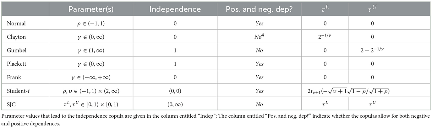
Table 1. Copula models.

2.2. Estimation methods

For the modeling strategy above, we focus on a semi-parametric copula model for each trading day t that combines a nonparametric model for marginal distribution with a parametric model for the copula. Based on Chen and Fan [26], we employ the two-stage maximum likelihood estimation (MLE) method to estimate this semi-parametric copula model for each trading day.

First, the parameters of the ARMA-EGARCH model for the individual return series on each trading day are estimated separately by MLE, and the marginal distributions of the estimated standardized intraday residuals are estimated by using the empirical marginal distributions.

Second, the parameters of a parametric copula are estimated by solving the following problem on every trading day t:

$\begin{array}{ll}{\widehat{\theta }}_t=arg{\displaystyle \underset{{\theta }_t}{max}}\frac{n}{1+n}{\displaystyle \sum _{j=1}^n}log{c}_t({\widehat{F}}_A({ẑ}_{A,t,j}),{\widehat{F}}_B({ẑ}_{B,t,j});{\theta }_t)& (10)\end{array}$

where c_t is the copula density function.

As detailed in Chen and Fan [26], the asymptotic distribution of the MLE of the copula parameter depend on the estimation error in the empirical marginal distributions of ẑ_i,t,j, and is unaffected by the estimated parameters in the ARMA-EGARCH model. Therefore, we ignore the estimation error from ARMA-EGARCH model for the copula estimation and inference. For the statistical inference on the estimated copula parameters, we adopt the bootstrap method as suggested by Chen and Fan [26] and Remillard [4] as follows:

  i. Use i.i.d. bootstrap to generate a bootstrap sample of the estimated standardized intraday residuals ẑ_i,t,j on each trading day t.

 ii. Transform each time series of bootstrap data using its empirical marginal distribution.

 iii. Estimate the copula model based on the transform data.

 iv. Repeat steps 1–3 with S times.

  v. Use the α/2 and quantiles of the distribution of estimated parameters to obtain a 1−α confidence interval for these parameters.

3. Data and descriptive statistics

There are three commodity futures exchanges in China: Zhenzhou Commodity Exchange (ZCE), Dalian Commodity Exchange (DCE) and Shanghai Futures Exchange (SFE). SFE is specialized in metal, energy and chemical-related futures while ZCE and DCE are specialized in agricultural commodity futures. We employ the high frequency data from Wind Financial Terminal for four agricultural commodity futures contracts in Chinese markets: white sugar, soybean, cotton and corn. Soybean and corn are traded in DCE while white sugar and cotton are traded in ZCE. The sample period is from 9 January 2006 to 28 November 2014 for all futures considered. The sample period allows us to analyze whether there have been important changes in the dynamics of dependence structure between agricultural commodity futures during the world food crisis (2007–2008) and the global financial crisis. We eliminate transactions executed during the weekends, public holidays and the days with low trading activity that could lead to estimation bias. After applying this elimination rule, we end up with 2,150 trading days in this study. Following Yang et al. [32], each agricultural commodity futures price series is constructed by rolling over the most liquid and active nearby futures contracts on the first trading day of the contract's expiration month and the prices of all futures are expressed in Chinese Yuan.

We follow the algorithm detailed in Barndorff-Nielsen et al. [33] to clean the high frequency data, and include only the observations for each trading day from 9:00 to 15:00 with a two-hour break between 11:30 and 13:30 and omit the overnight observations so as to reduce the effect of asynchronous trading. In order to obtain regularly spaced observations, we adopt the calendar time sampling and the last-tick interpolation method. We use the 5-min sampling frequency in an attempt to strike a reasonable balance between two potential effects: at very high sampling frequency, we confront a positive bias as detailed in Nelson [34], and at too low sampling frequency, we end up with a small sample and face a positive in estimating the intraday dependence.

Figure 1 shows the evolution of four agricultural commodity futures prices at 5-min frequency. It follows that the prices in all four futures appear to move in a similar fashion, with a big spike in 2008 when the food price crisis occurred, and a sharp increase between 2010 and 2011. Figure 2 further displays the 5-min and daily log returns time series of the four agricultural futures. The j^th 5-min intraday log returns for asset i on trading day t are obtained as r_i,t,j = 100 × (p_i,t,j−p_i,t,j−1), where p_i,t,j is the j^th log price sampled at 5-min frequency on trading day t for asset i. Our daily returns are simply computed as a sum of 5-min intraday log returns, $r_{i,t}={\displaystyle \sum _{j=1}^n{r}_{i,t,j}}$. From Figure 2, we can see that the volatility of returns for both daily and 5-min intraday data is time-varying, with significant fluctuations during the period of 2007–2008 and 2010–2011.

FIGURE 1

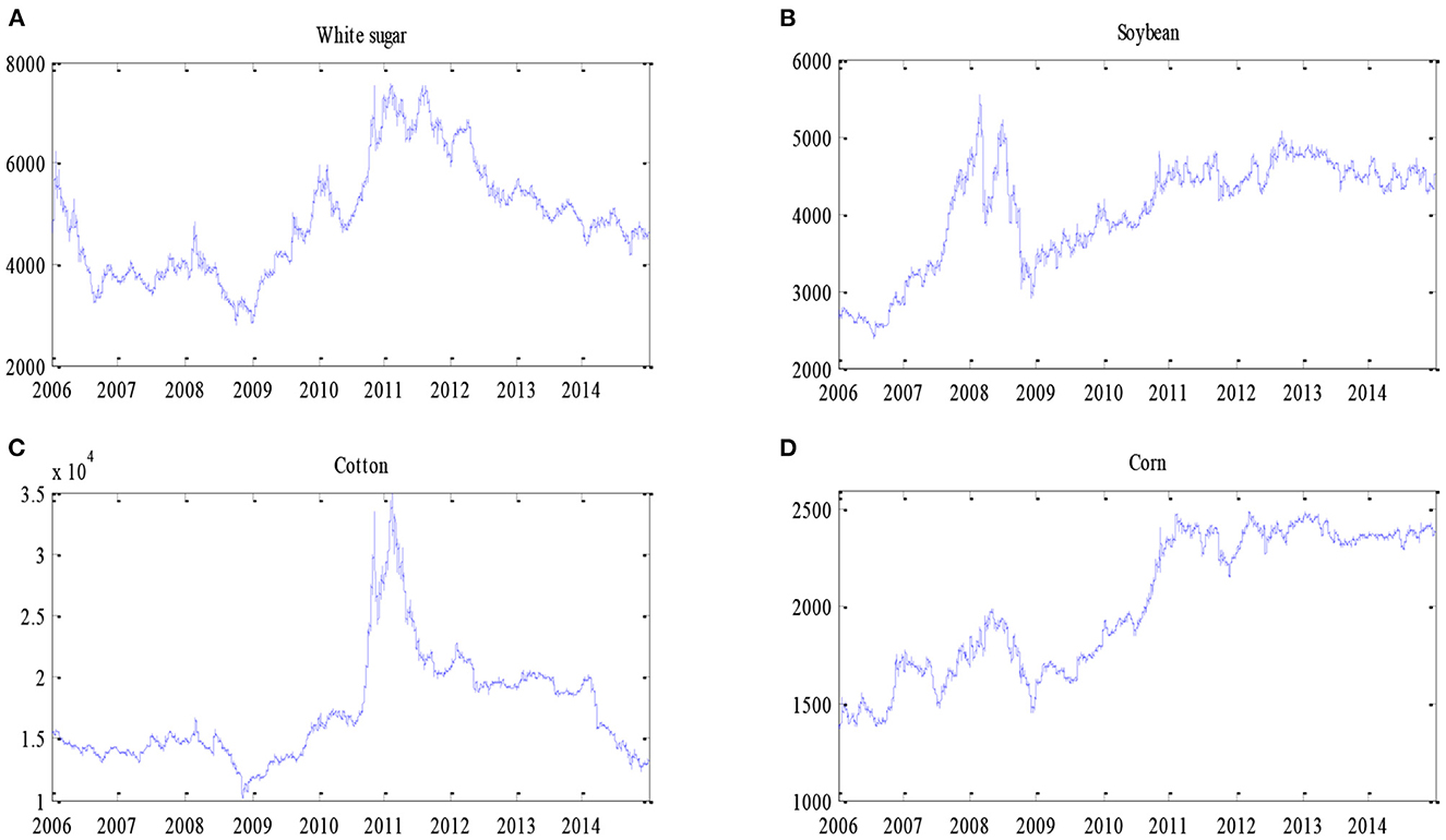
Figure 1. White sugar (A), soybean (B), cotton (C), and corn (D) futures prices at 5 min frequency.

FIGURE 2

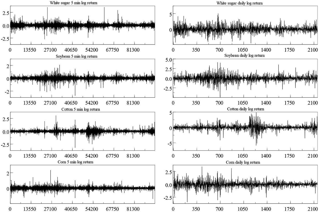
Figure 2. Return series of four agricultural commodity futures.

Table 2 reports the descriptive statistics of the agricultural commodity futures return series and the estimated standardized residuals from ARMA-EGARCH model at daily and 5-min sampling frequencies. The means of all returns series and residual series at both daily and 5-min sampling frequencies are close to zero and the corresponding standard deviations are greater in an order of several magnitudes, implying no significant trend in the data. The standard deviations of residual series at both daily and 5-min sampling frequencies are greater than those of the returns series. The return series for all agricultural commodity futures at 5-min sampling frequencies tend to have smaller standard deviations than the daily returns. However, the estimated standardized residuals from the ARMA-EGARCH model display the reverse characteristics. All series display high values for the kurtosis statistics consistent with fat tails in their distributions, and the estimated standardized residuals tend to have thinner tail⁴ than the returns at both daily and 5-min sampling frequency. For all series at both daily and 5-min sampling frequencies, both skewness and kurtosis indicate that these series are not normally distributed, and thus we need the copula approach.

TABLE 2

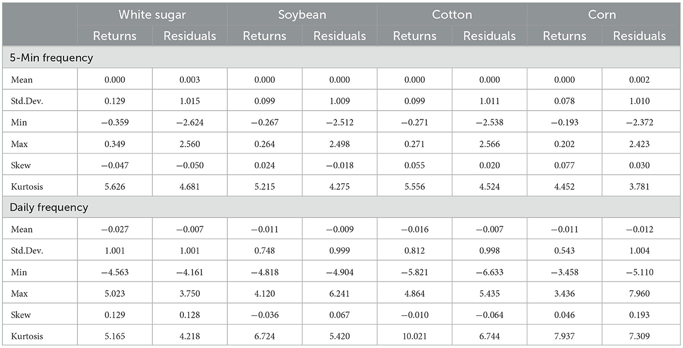
Table 2. Descriptive statistics.

4. Empirical results

4.1. Preliminary analysis

As discussed in Andersen and Bollerslev [35], it is important to consider intraday seasonality before using standard volatility models for the intraday returns. However, we find that the seasonality correction removes the extreme tail observations which are important for the copula estimation. In addition, the marginal distribution model in this paper for the conditional mean and variance is estimated by using intraday returns on each trading day and this provides some forms of adjustments for the intraday seasonality pattern. Therefore, we decide not to make seasonal adjustment for the intraday returns before passing through the ARMA-EGARCH filter in our research.

Figure 3 displays the daily realized correlation as suggested in Barndorff-Nielsen and Shephard [27] and the intraday dependence estimator based on Gaussian copula for each pair of agricultural commodity futures for a period from 9 January 2006 to 28 November 2014 by using 5-min sampling frequency. The red line is the daily realized correlation while the blue line is the Gaussian copula intraday dependence. The realized correlation between each two agricultural commodity futures A and B for a given day t is computed in the usual way:

$\begin{array}{ll}RCor{r}_t=\frac{{\displaystyle \sum _{j=1}^n}{r}_{A,t,j}{r}_{B,t,j}}{\sqrt{{\displaystyle \sum _{j=1}^n}{r}_{A,t,j}^2{\displaystyle \sum _{j=1}^n}{r}_{B,t,j}^2}}& (11)\end{array}$

where n is the number of 5-min returns on a trade day, $\sqrt{{\displaystyle \sum _{j=1}^n{r}_{A,t,j}^2}}$ is the daily realized volatility for futures A.

FIGURE 3

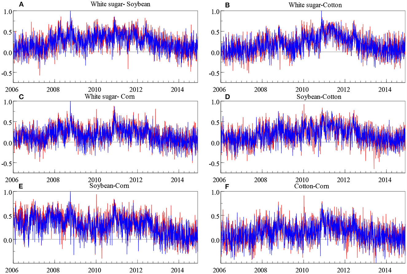
Figure 3. Realized correlation (red line) and the intraday dependence (blue line) of white sugar-soybean (A), white sugar-cotton (B), white sugar-corn (C), soybean-cotton (D), soybean-corn (E), and cotton-corn (F).

As we can see in Figure 3, for all pairs of agricultural commodity futures, the Gaussian copula intraday dependence and the realized correlation are closely following each other. This indicates that the dependence between agricultural commodity futures is preserved after the univariate ARMA-EGARCH filtration. The dependence of each agricultural commodity futures pair varies significantly over time, with an increase after the food price crisis of 2007–2008 and a steady decrease during the period 2013–2014.

To illustrate the advantage of using the high-frequency data, we use the pair of white sugar-soybean futures as an example. Figure 4 presents the scatter plots of the intraday residuals in three days (9 January 2006, 1 August 2007, and 9 October 2008) and the daily residuals during period of 2006–2008 for the white sugar-soybean pair. On 9 January 2006, the scatter plot is relatively elliptical and shows little tail dependence. However, the plots on 1 August 2007 and 9 October 2008 show that the dependence between the white sugar-soybean pair is evident. These variations in the dependence over time cannot be captured based on daily data as shown in the plot of the daily residuals in Figure 4.

FIGURE 4

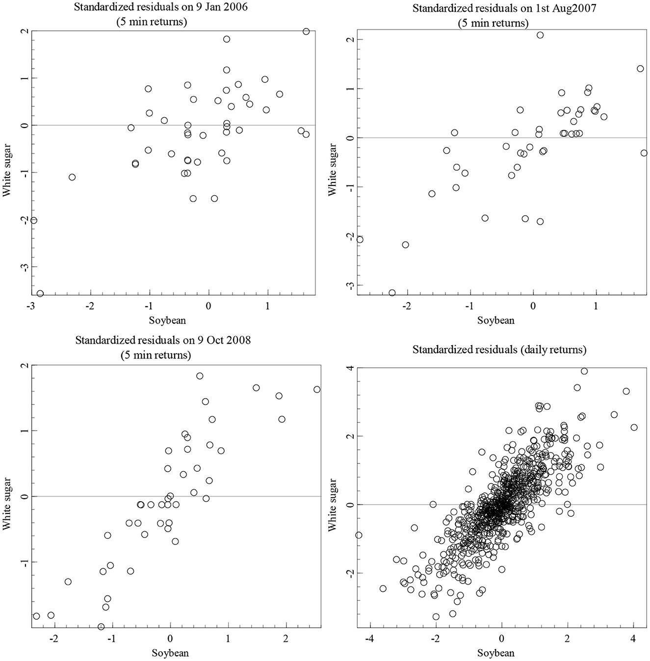
Figure 4. Scatter plots of 5-min and daily residuals for white sugar-soybean pair.

4.2. Model selection

In order to investigate the dependence between the agricultural commodity futures in China, we estimate the dependence estimation (${\widehat{\theta }}_t$) results of the SCBMD model based on the high frequency data implemented on each trading day as detailed in Section 2. Further, we examine the evolution of daily dependence between agricultural commodity futures by contrasting with the constant unconditional dependence estimator (${\widehat{\theta }}_t^{con}$), the rolling window dependence estimator (${\widehat{\theta }}_t^{RW}$) and the autoregressive dependence estimator (${\widehat{\theta }}_t^{AR}$). The constant unconditional dependence estimator is obtained by estimating the SCBMD model over the whole daily return series. The rolling window estimator is calculated by estimating the SCBMD model over a rolling window of 100 daily return observations. The autoregressive estimator is based on Patton [36].

For each pair of agricultural commodity futures, we estimate seven copula models as discussed in Section 2, and select the two copulas that give the two greatest average log likelihoods. Table 3 reports the average log likelihood estimates of the six agricultural commodity futures pairs. We find that the Student's-t copula and the SJC copula significantly outperform all five other models for all six pairs of agricultural commodity futures. Further, we use the Student's-t copula and the SJC copula to estimate ${\widehat{\theta }}_t$, ${\widehat{\theta }}_t^{con}$, ${\widehat{\theta }}_t^{RW}$, and ${\widehat{\theta }}_t^{AR}$ for each pair of agricultural futures. We use the dependence estimators (ρ) from the Student's-t copula and tail dependence estimators (upper tail dependence τ^Uand lower tail dependence τ^L) from the SJC copula to investigate the dependence and tail dependence between each pair of agricultural futures respectively.

TABLE 3

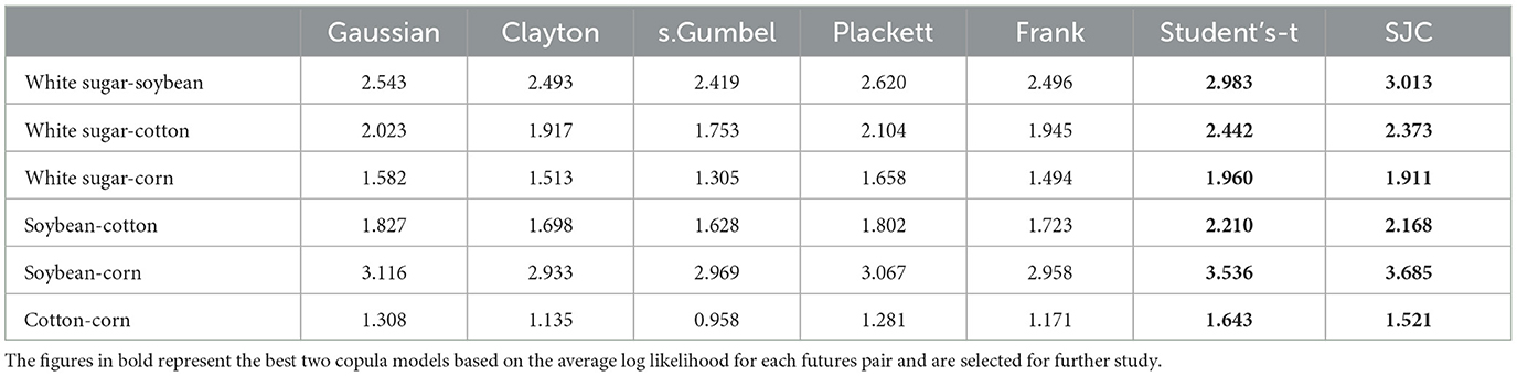
Table 3. Average log likelihood for the seven copulas.

As the effects of time aggregation of the ARMA-EGARCH model is limited and can be ignored [see 5, 34, 37], the proposed intraday dependence estimator is a good estimator for time-varying dependence. In order to deal with the multiple sources of possible biasness simultaneously in the intraday dependence estimator, motivated by Martens et al. [38], we estimate the rescaling factor a_f by using the mean of ${\widehat{\theta }}_t$/${\widehat{\theta }}_t^{con}$ estimated in the initial 100 trading days, i.e., between 9 January 2006 and 26 June 2006, and assume that it remains constant throughout the remaining period to adjust the intraday dependence estimator by ${\widehat{\theta }}_t^{*}={\widehat{\theta }}_t/a_f$ over the period of 27 June 2006 through 28 November 2014 (totally 2050 trading days).

4.3. Daily dependence

Figure 5 shows the evolution of the estimated dependence measure ρ for the Student's-t copula and tail dependence measures τ^U and τ^L for the SJC copula with the constant unconditional dependence estimator (black dotted horizontal lines), intraday dependence estimator (red dotted lines), rolling window estimator (blue solid lines) and autoregressive estimator (black solid lines). Some key points need to be highlighted. First, the dependence between all pairs of agricultural commodity futures is dynamic, and the time-varying copula parameters tend to trend together. Second, the intraday dependence estimator for each pair of agricultural commodity futures tends to be more volatile than other estimators. Third, in general, the intraday dependence estimator for each pair of agricultural commodity futures tends to be lower than other estimators in most trading days, but increases dramatically during the crisis periods (the world food crisis of 2007–2008 and the global financial crisis of 2008–2011). This shows how the intraday dependence estimator effectively reflects the increasingly occurrence in risk quickly when agricultural commodity futures have large negative dependence.

FIGURE 5

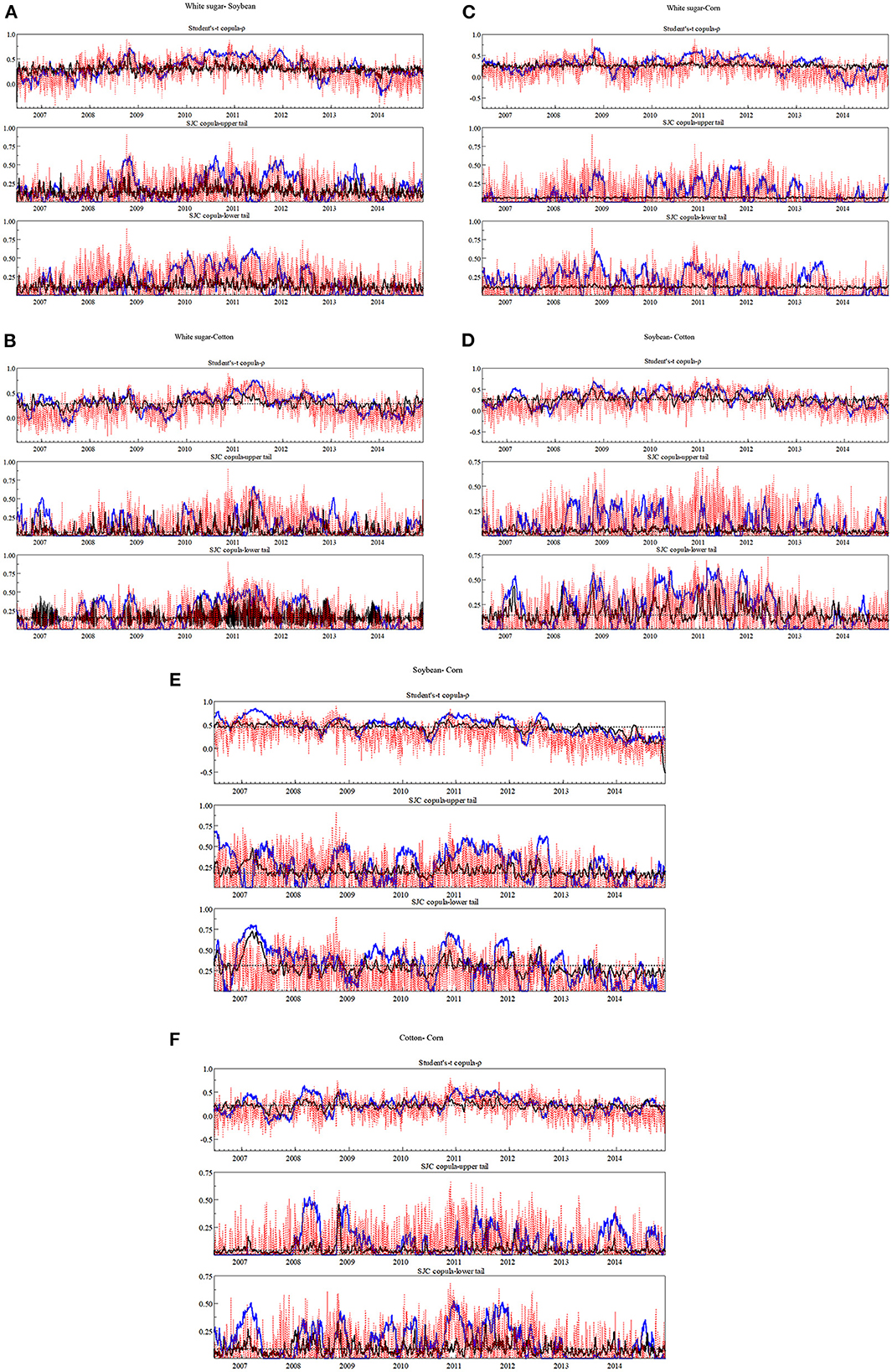
Figure 5. Evolution of the estimated dependence of white sugar-soybean (A), white sugar-cotton (B), white sugar-corn (C), soybean-cotton (D), soybean-corn (E), and cotton-corn (F). Measure ρ for the Student's-t copula and tail dependence measures τ^U and τ^L for the SJC copula with the constant unconditional dependence estimator (black dotted horizontal lines), intraday dependence estimator (red dotted lines), rolling window estimator (blue solid lines) and autoregressive estimator (black solid lines).

In order to observe the time-varying dependence structure between each pair of agricultural commodity futures more clearly and to assess the effects of crisis, Table 4 reports the mean of all dependence measures (ρ_t, ${\tau }_t^U$, and ${\tau }_t^L$) and its corresponding standard deviations for whole sample period and four sub-periods: (i) June 2006-December 2006, (ii) January 2007-August 2008 (the world food crisis), (iii) September 2008-December 2011 (global financial crisis), and (iv) January 2012-November 2014. As suggested in Patton [36], Table 4 also reports the mean of average tail dependence measure (defined as $({\tau }_t^U+{\tau }_t^L)/2$) with its corresponding standard deviations, and the mean of the difference between the upper and lower tail dependence measures (defined as ${\tau }_t^U-{\tau }_t^L$), which describes the degree of asymmetry, with its corresponding standard deviation for each periods.

TABLE 4

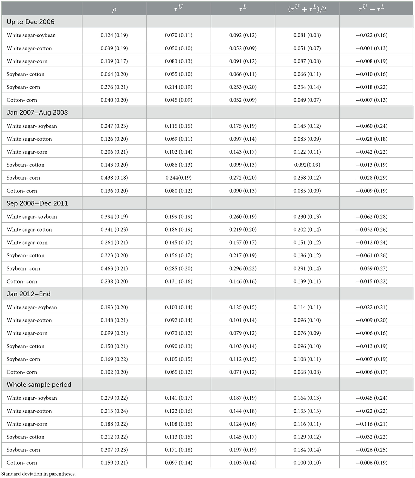
Table 4. Mean of dependence measures and its corresponding standard deviations for whole sample period and four sub-periods.

Figures 5A–C illustrate the changes in the dependence and tail dependence between white sugar future and other three agricultural futures. Their overall pattern is quite similar as they show a sharp increase in ρ_t during the two crisis periods (the world food crisis period and the global financial crisis period) relative to the period of June 2006-December 2006, and then a sharp decrease relative to these two crisis periods during January 2012-November 2014. More specifically, regarding the white sugar-soybean futures pair, the average dependence tends to strengthen in the middle of 2007 (${\bar{\rho }}_{06}\cong 0.12$, ${\bar{\rho }}_{07-08}\cong 0.25$), which is still less than the average dependence level for whole sample period, and clearly further strengthens during the global financial crisis period (${\bar{\rho }}_{08-11}\cong 0.39$), which is more than the average dependence level for whole sample period, and then weakens to below the overall average dependence level during the last period (${\bar{\rho }}_{12-14}\cong 0.19$). The average dependence results are quite similar for the white sugar-corn futures pair (${\bar{\rho }}_{06}\cong 0.14$, ${\bar{\rho }}_{07-08}\cong 0.21$, ${\bar{\rho }}_{08-11}\cong 0.26$, ${\bar{\rho }}_{12-14}\cong 0.10$). In contrast, the dependence strength (ρ_t) between the white sugar-cotton futures pair goes from being almost nonexistent during the first period (${\bar{\rho }}_{06}\cong 0.04$) to relatively strong and positive during the period of the world food crisis (${\bar{\rho }}_{07-08}\cong 0.13$) and clearly further strengthen during the global financial crisis period (${\bar{\rho }}_{08-11}\cong 0.34$), and then sharply weakens during the last period (${\bar{\rho }}_{12-14}\cong 0.10$). From the results of the average tail dependence ($({\tau }_t^U+{\tau }_t^L)/2$) as reported in Table 4, we confirm that the changing pattern of the dependence strength (ρ_t) between the white sugar futures and other three agricultural commodity futures also take place in tail dependence. More specifically, regarding the white sugar-soybean futures pair, the average tail dependence goes from being relatively weak during the first period (${\bar{\tau }}_{06}\cong 0.08$) to relatively strong during the world food crisis period (${\bar{\tau }}_{07\mathrm{\text{-}}08}\cong 0.15$), and clearly further strengthen during the global financial crisis period (${\bar{\tau }}_{08\mathrm{\text{-11}}}\cong 0.23$), and then sharply weakens during the last period (${\bar{\tau }}_{12\mathrm{\text{-}}14}\cong 0.11$). The results of the average tail dependence are quite similar for the white sugar-cotton future pair (${\bar{\tau }}_{06}\cong 0.05$,${\bar{\tau }}_{07\mathrm{\text{-}}08}\cong 0.08$, ${\bar{\tau }}_{08\mathrm{\text{-11}}}\cong 0.20$, ${\bar{\tau }}_{12\mathrm{\text{-}}14}\cong 0.10$) and white sugar-corn future pair (${\bar{\tau }}_{06}\cong 0.09$, ${\bar{\tau }}_{07\mathrm{\text{-}}08}\cong 0.12$,${\bar{\tau }}_{08\mathrm{\text{-11}}}\cong 0.15$,${\bar{\tau }}_{12\mathrm{\text{-}}14}\cong 0.08$). From the results of average asymmetric degree measured by the mean of the difference between the upper and lower tail dependence measures (${\tau }_t^U-{\tau }_t^L$) as reported in Table 4, we find that, for white sugar-soybean, white sugar-cotton, and white sugar-corn futures pairs, the upper tail dependence is less than the lower tail dependence during all four periods, implying that the white sugar is more dependent on the other three agricultural commodity futures during the upward market condition than downward market condition, and the degree of asymmetric strengthens during the two crisis periods.

Figures 5D, E report the changes in the dependence and tail dependence between the soybean and cotton futures, and the soybean and corn futures. The overall pattern of the dependence strength (ρ_t) between these two future pairs show a sharp increase during the world food crisis period (${\bar{\rho }}_{06}\cong 0.06,0.38$ and ${\bar{\rho }}_{07-08}\cong 0.14,0.44$ respectively) and further increase in the global financial crisis period (${\bar{\rho }}_{08-11}\cong 0.32,0.46$ respectively), and then a clearly decrease during the last period (${\bar{\rho }}_{12-14}\cong 0.15,0.17$ respectively). Similarly to the dependence strength, the overall pattern of the average tail dependence between these two futures pairs also tends to strengthen during the two crisis periods, and clearly weakens during the last period. The upper tail dependence between these two futures pairs are less than the lower tail dependence during all four periods, and the asymmetric degree also strengthen during the two crisis periods. Figure 5F reports the changes in the dependence and tail dependence between the cotton and corn futures. Similar observations can be made for this pair of futures.

Comparing the average dependence measures for all pairs of agricultural commodity futures, we find that both the average dependence and the average tail dependence between the soybean and corn futures display higher values than those between other pairs for whole sample period and all four sub-periods. Moreover, the average asymmetric degree between the white sugar and soybean pair show a higher value than this between the other pairs for whole sample period and all four sub-periods.

Finally, unlike the dependence strength (ρ_t) and the average tail dependence ($({\tau }_t^U+{\tau }_t^L)/2$) themselves, their volatility remain quite stable for all future pairs considered over the four periods while the standard deviations of the difference between the upper and the lower tail dependence are quite heterogeneous across different periods. However, the standard deviations of the dependence strength and the average tail dependence are also quite heterogeneous across different future pairs.

In summary, the above analysis uncovers several stylized facts. First, each agricultural futures pair exhibits average positive time-varying dependence for most of the time, indicating that agricultural commodity futures dynamically co-move with different intensity. In fact, the estimations in this paper show that the dependence between these agricultural commodities futures are best captured by a relationship that varies over time while being slightly asymmetric in tail dependence. That is, we find relative strong average tail dependence between each agricultural commodity futures pair during all four periods considered, especially during the two crisis periods, and the upper tail dependence between each agricultural future pair is less than the lower tail dependence for most of the time. In average, the dependence between soybean-corn pair is the strongest in all six pairs of agricultural futures.

Second, we find that the dependence between these agricultural commodity futures has clearly increased during the world food crisis in 2007–2008 and the global financial crisis in 2008–2011, and this change also takes place in tail dependence with its asymmetry. In an economic sense, the futures prices tend to co-move more not only during the period of underlying asset crisis i.e. food crisis, but also during the period of financial crisis. In fact, we find that the intensity of the dependence differs relying on the period considered. During the first period considered, agricultural commodity futures tend to show on average almost no relationship or relative weak relationship, with the exception of the pair of soybean-corn futures that shows a strong dependence during this period. Then, we discover a stronger dependence for all agricultural future pairs during the world food crisis and the global financial crisis period, and the average tail dependence between these agricultural commodity futures with its asymmetry also increases during these two crisis periods. The finding that the dependence measure between all agricultural futures pairs unambiguous increases indicate a growing integration between these agricultural futures markets. These growing dependences may be due to so called “financialization” of agricultural markets and higher volume of agricultural commodity futures contracts traded in China in 2008–2011. Following the global financial crisis, many investors shifted from mortgage markets to agriculture commodities. This higher activity in financial agricultural markets in China may be further stimulating dependence in price returns between agricultural futures.

Third, the intraday dependence estimator (red dotted lines in Figure 5) tends to be more volatile than the constant unconditional dependence estimator (black dotted horizontal lines), rolling window estimator (blue solid lines), and autoregressive estimator (black solid lines). The intraday dependence estimator effectively reflects the quickly increasement in risk during the time when agricultural commodity futures have high negative dependence. These results indicating that the intraday dependence estimated with high-frequency data better identify the dynamic interactions between futures prices, which can be smoothed by the long-time window or rolling method used by the other estimators. Therefore, intraday dependence estimator provides more information for short-term especially the intraday trader.

4.4. Intraday dependence

Many studies have concentrated on the intraday patterns of volatilities based on intraday data. Andersen and Bollerslev [35] and Tsay [39], find that the intraday volatility typically exhibit a U-shape, i.e., higher during the opening and closing hours and lower around the midday. Similar the effects have been documented for other measures of intraday trading activity such as bid-ask spreads (e.g., [40]), various types of durations (e.g., [41]) and transaction volumes (e.g., [42]). However, fewer studies have worked on the intraday pattern of the dependence structure between the assets. In this section, we consider the intraday dependence patterns in Chinese agricultural futures markets. Following Bubak et al. [43], we first compute the intraday realized correlation, which can give us a preliminary understanding of the intraday dependence patterns. For further understanding of the intraday dependence patterns, we estimate the SCBMD model, as detailed in Section 2.

Figure 6 displays the evolution of the intraday realized correlation for each of the six pairs of agricultural commodity futures. Particularly, it shows the evolution of the average 30-min realized correlation, calculated by averaging the intraday realized correlation over 30-min intraday intervals during the whole sample period. One can observe a lopsided inverted U-shaped pattern for the intraday realized correlation between almost all pairs of agricultural commodity futures. Notably, the peak of the average 30-min realized correlations for all pairs occur during midday (13:35–14:00), and the average 30-min realized correlations around the closing time (14:35–15:00) tend to be much lower than those of other trading times. Thus, the intraday dependence between each pair of agricultural commodity futures is much stronger around midday and much weaker around the closing time than other trading time.

FIGURE 6

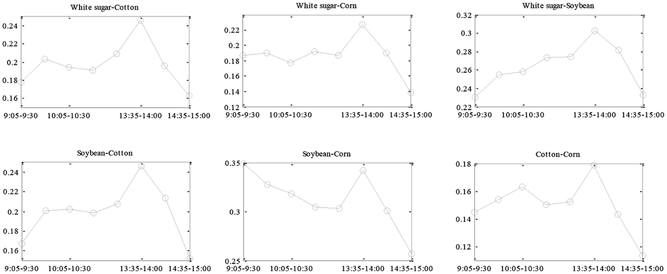
Figure 6. The evolution of average intraday realized correlation. The intraday realized correlation is computed over 30-min intraday intervals and then averaged across each interval over the whole sample.

To further assess this specific intraday pattern, we both consider the constant unconditional dependence estimators and the average of the autoregressive dependence estimators at a given sampling time point over the sample period. The constant unconditional dependence estimators are obtained by using the SCBMD model over the whole time series of each intraday return, while the autoregressive dependence estimators are calculated by using the SCBMD model with AR specification based on Patton [36]. Figure 7 plots the average dependence estimators from the Student's-t copula and the average tail dependence estimators from the SJC copula for each of the six pairs of agricultural futures.

FIGURE 7

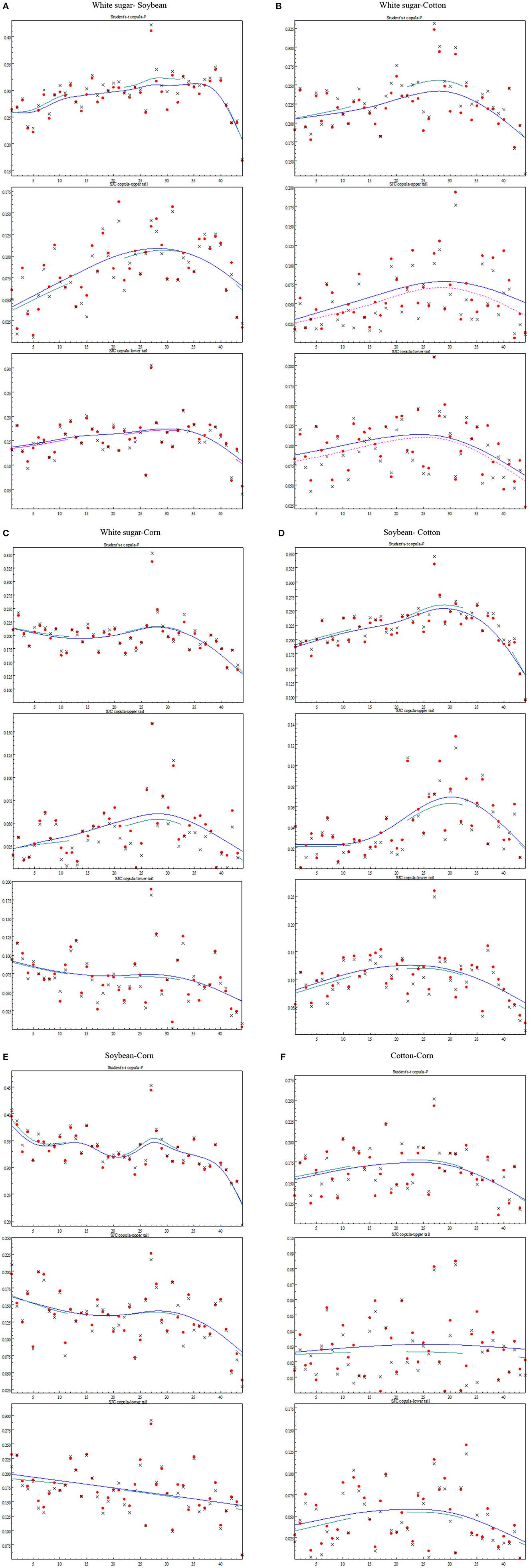
Figure 7. The evolution of intraday dependence estimator of white sugar-soybean (A), white sugar-cotton (B), white sugar-corn (C), soybean-cotton (D), soybean-corn (E), and cotton-corn (F). For a given time point, we consider the time series of returns at this point over the sample period. The black points marked with x are the constant unconditional dependence estimators using the SC BMD model. The red dotted points are the average of the autoregressive dependence estimators using the SCBMD model with AR specification based on Patton [36]. Using the cubic spline method, we smooth the constant unconditional dependence estimators to obtain the blue solid lines and the average of the autoregressive dependence estimators to obtain the red dotted lines.

Similar to the results of the average 30-min intraday realized correlation, both the overall dependence estimators and (upper- and lower-) tail dependence estimators exhibit a lopsided inverted U-shaped pattern for almost all pairs of agricultural commodity futures based on either the unconditional estimators or the averaged autoregressive estimators. To be more specific, we find that the average dependence and the average tail dependence tend to be low around the opening time, and then increase gradually until reaching the peaks around the midday, after which they tend to decrease until the closing time. This intraday dependence pattern is evident for nearly all pairs of agricultural futures.

This specific intraday pattern for the dependence structure between the pairs of the agricultural commodity futures can be explained by the flow of information during a trading day. First, the opening hours are normally dominated by idiosyncratic effects with little surprises, resulting in the lower dependence level. In particular, a relatively higher percentage of idiosyncratic and sector-specific news is impounded at the opening of the trading day. Such idiosyncratic components may play a dominant role around the opening hours, which result in lower levels of dependence between agricultural commodity futures. Second, the influences of the market-wide information such as macro-economic announcements are more likely to increase as the trading proceeds. The market mode components can eventually play a dominant role around the midday. Thus the dependence level is likely to increase after the opening time and reach a peak around the midday. Third, idiosyncratic components may become dominant again around the closing time. In particular, as discussed in Bibinger et al. [44], in order to limit the (overnight) risk, many traders tend to unwind their inventory positions that are built up over the trading day after midday. Hence, the idiosyncratic effects become stronger and stronger after the midday until the closing time. This can lead to the decreasing of dependence after the midday and the dependence at the end of the day is therefore likely the lowest in the afternoon trading session. The intraday pattern of the dependence structure between soybean-corn futures pair is slightly different, i.e., the dependence level is relatively higher than other futures pairs during the opening hours. The reason for this difference may be due to the relatively higher substitution effect between soybean and corn.

5. Concluding remarks

Difference from the previous studies which mainly focus on the relationship between the spot and the futures prices for agricultural commodities, This paper examines the daily and intraday dependence structure between the agricultural commodity futures in China by employing the semi-parametric copula models and high frequency data. In contrast to various versions of the multivariate GARCH models widely used in the literature, the semi-parametric copula model estimated with the high frequency data provides a flexible and comprehensive description of the dependence between the agricultural futures, and allows us to observe the latent conditional dependence as well as the intraday dependence patterns between each pair of agricultural futures.

The empirical results show that each pair of agricultural commodity futures exhibits positive time-varying dependence for most of the time, indicating that agricultural commodity futures dynamically co-move with different intensities. We also find the relatively strong tail dependence between each pair of agricultural commodity futures during all four sub-periods considered, especially during the world food crisis and the global financial crisis. We also find that the upper tail dependence between each pair of agricultural futures is less than the lower tail dependence for most of the time. The overall dependence as well as (upper and lower) tail dependence between these pairs of agricultural commodity futures has increased significantly during the world food crisis and the global financial crisis. Moreover, the intraday dependence between each pair of the agricultural commodity futures exhibits a lopsided inverted U-shaped pattern in most cases with relatively lower dependence levels around the opening and the closing time, and a peak around the midday. This special intraday dependence pattern between the agricultural futures may be due to the existence of more idiosyncratic components during the opening and closing hours of trading and more market mode components during the midday. This paper only explores the dynamic dependence between agricultural futures, the possible underlying determinants of this dynamics like trading micro-structure [45], the possible information content of dependence or correlations [46] or behavior characteristic like herding [6, 47] are further extensions. The semi-parametric copula model with high-frequency data applies to the dependence structure of general commodity futures such as gold and silver, whose dynamics may show a different pattern due to price behavior of its underlying assets.

Data availability statement

The original contributions presented in the study are included in the article/supplementary material, further inquiries can be directed to the corresponding author.

Author contributions

The author confirms being the sole contributor of this work and has approved it for publication.

Conflict of interest

The author declares that the research was conducted in the absence of any commercial or financial relationships that could be construed as a potential conflict of interest.

Publisher's note

All claims expressed in this article are solely those of the authors and do not necessarily represent those of their affiliated organizations, or those of the publisher, the editors and the reviewers. Any product that may be evaluated in this article, or claim that may be made by its manufacturer, is not guaranteed or endorsed by the publisher.

Footnotes

1. ^During 2007–2008 food prices rose dramatically worldwide, creating a global food crisis and causing political and economic instability and social unrest in both poor and developed countries. Between early 2006 and 2008, the average world price for rice rose by 217%, wheat by 136%, maize by 125% and soybeans by 107% respectively. In late April 2008, rice prices hit 24 cents a pound, twice the price that it was seven months earlier. See http://www.world-crisis.net/food-crisis.html, accessed on 16 January, 2016.

2. ^Gilbert [10] find that the prices of various agricultural commodities regularly move together although there are many different causes that give rise to the increases (and fluctuations) of agricultural commodity prices.

3. ^See https://fimag.fia.org/articles/2014-fia-annual-global-futures-and-options-volume-gains-north-america-and-europe-offset, accessed on 16 January, 2016.

4. ^Although the Clayton copula allows for negative dependence for γ ∈ (−1, 0), the form of this dependence is different from the positive dependence case (γ > 0), and is not generally used in empirical works.

References

1. Gardebroek C, Hernandez MA, Robles LM. Market interdependence and volatility transmission among major crops. Agric Econ. (2016) 47:141–55. doi: 10.1111/agec.12184

CrossRef Full Text | Google Scholar

2. Hernandez M, Torero M. Examining the dynamic relationship between spot and future prices of agricultural commodities (No. 988). Washington, DC: International Food Policy Research Institute (IFPRI). (2010).

Google Scholar

3. Von Ledebur O, Schmitz J. Corn Price Behavior—Volatility Transmission During the Boom on Futures Markets. In: 113th EAAE Seminar “A Resilient European Food Industry and Food Chain in a Challenging World.” (Crete: European Association of Agricultural Economists) (2009) p. 3–6.

Google Scholar

4. Rémillard B. Goodness of fit tests for copulas of multivariate time series. Econometrics, MDPI. (2017) 5:1–3.

Google Scholar

5. Alexander C, Lazar E. On the continuous limit of GARCH. Discussion Papers in Finance, ICMA Centre, University of Reading. Reading, UK: ICMA Centre, The University of Reading (2005). doi: 10.2139/ssrn.569081

CrossRef Full Text | Google Scholar

6. Sibande X, Gupta R, Demirer R, Bouri E. Investor sentiment and (anti) herding in the currency market: evidence from twitter feed data. J Behav Finance. (2023) 24: 56–72. doi: 10.1080/15427560.2021.1917579

CrossRef Full Text | Google Scholar

7. Loh L. Co-movement of Asia-Pacific with European and US stock market returns: a cross-time-frequency analysis. Res Int Bus Finance. (2013) 29:1–13. doi: 10.1016/j.ribaf.2013.01.001

CrossRef Full Text | Google Scholar

8. Kiviaho J, Nikkinen J, Piljak V, Rothovius T. The co-movement dynamics of European frontier stock markets. Eur Financial Manag. (2014) 20:574–95. doi: 10.1111/j.1468-036X.2012.00646.x

CrossRef Full Text | Google Scholar

9. Zhang B, Li XM. Has there been any change in the comovement between the Chinese and US stock markets? Int Rev Econ Finance. (2014) 29:525–536. doi: 10.1016/j.iref.2013.08.001

CrossRef Full Text | Google Scholar

10. Gilbert CL. How to understand high food prices. J Agri Eco. (2010) 61:398–425. doi: 10.1111/j.1477-9552.2010.00248.x

CrossRef Full Text | Google Scholar

11. Serra T. Volatility spillovers between food and energy markets: a semi-parametric approach. Energy Econ. (2011) 33:1155–64. doi: 10.1016/j.eneco.2011.04.003

CrossRef Full Text | Google Scholar

12. Du X, Cindy LY, Hayes DJ. Speculation volatility spillover in the crude oil and agricultural commodity markets: a Bayesian analysis. Energy Econ. (2011) 33:497–503. doi: 10.1016/j.eneco.2010.12.015

CrossRef Full Text | Google Scholar

13. Nazlioglu S, Erdem C, Soytas U. Volatility spillover between oil and agricultural commodity markets. Energy Econ. (2013) 36:658–65. doi: 10.1016/j.eneco.2012.11.009

PubMed Abstract | CrossRef Full Text | Google Scholar

14. Mensi W, Beljid M, Boubaker A, Managi S. Correlations volatility spillovers across commodity and stock markets: Linking energies, food, and gold. Econ Model. (2013) 32:15–22. doi: 10.1016/j.econmod.2013.01.023

CrossRef Full Text | Google Scholar

15. Creti A, Joëts M, Mignon V. On the links between stock and commodity markets' volatility. Energy Econ. (2013) 37:16–28. doi: 10.1016/j.eneco.2013.01.005

PubMed Abstract | CrossRef Full Text | Google Scholar

16. Abdelradi F, Serra T. Asymmetric price volatility transmission between food and energy markets: the case of Spain. Agric Econ. (2015) 46:503–13. doi: 10.1111/agec.12177

CrossRef Full Text | Google Scholar

17. Le Pen Y, Sevi B. Revisiting the Excess Co-Movement of Commodity Prices in a Data Rich Environment. (2010). Available online at: http://ideas.repec.org/p/dau/papers/123456789-6800.html

Google Scholar

18. Zhao J, Goodwin B. Volatility Spillovers in Agricultural Commodity Markets: An Application Involving Implied Volatilities from Options Markets. In: Selected Paper prepared for presentation at the AAEA and NAREA Joint Annual Meeting, Pittsburgh, Pennsylvania. (2011) p. 24–26.

Google Scholar

19. Lahiani A, Nguyen DK, Vo T. Understanding return and volatility spillovers among major agricultural commodities. J Appl Busi Res. (2013) 29:1781–90. doi: 10.19030/jabr.v29i6.8214

CrossRef Full Text | Google Scholar

20. Ling S, McAleer M. Asymptotic theory for a vector ARMA-GARCH model. Econ Theory. (2003) 19:280–310. doi: 10.1017/S0266466603192092

CrossRef Full Text | Google Scholar

21. Beckmann J, Czudaj R. Volatility transmission in agricultural futures markets. Econ Model. (2014) 36:541–6. doi: 10.1016/j.econmod.2013.09.036

PubMed Abstract | CrossRef Full Text | Google Scholar

22. Hernandez MA, Ibarra R, Trupkin DR. How far do shocks move across borders? Examining volatility transmission in major agricultural futures markets. Eur Rev Agric Econ. (2014) 41:301–25. doi: 10.1093/erae/jbt020

CrossRef Full Text | Google Scholar

23. Ji Q, Bouri E, Roubaud D, Shahzad S. Risk spillover between energy and agricultural commodity markets: a dependence-switching covar-copula model. Energy Econ. (2018) 75:14–27. doi: 10.1016/j.eneco.2018.08.015

PubMed Abstract | CrossRef Full Text | Google Scholar

24. Mensi W, Tiwari A, Bouri E, Roubaud D, Al-Yahyaee KH. The dependence structure across oil, wheat, and corn: a wavelet-based copula approach using implied volatility indexes. Energy Econ. (2017) 66:122–39. doi: 10.1016/j.eneco.2017.06.007

CrossRef Full Text | Google Scholar

25. Cheung CS, Miu P. Diversification benefits of commodity futures. J Int Financial Mark Inst. (2010) 20:451–74. doi: 10.1016/j.intfin.2010.06.003

CrossRef Full Text | Google Scholar

26. Chen X, Fan Y. Estimation model selection of semi-parametric copula-based multivariate dynamic models under copula misspecification. J Econom. (2006) 135:125–54. doi: 10.1016/j.jeconom.2005.07.027

CrossRef Full Text | Google Scholar

27. Barndorff-Nielsen OE, Shephard N. Econometric analysis of realized covariation: High frequency based covariance, regression, and correlation in financial economics. Econometrica. (2004) 72:885–925. doi: 10.1111/j.1468-0262.2004.00515.x

CrossRef Full Text

28. Sklar A. Fonctions de Riépartition á n Dimensions et Leurs Marges. Paris: Publications de l'Institut Statistique de l'Université de Paris. (1959) p. 229–31.

Google Scholar

29. Longin F, Solnik B. Extreme correlation of international equity markets. J Finance. (2001) 56:649–76. doi: 10.1111/0022-1082.00340

CrossRef Full Text | Google Scholar

30. Delatte AL, Lopez C. Commodity equity markets: Some stylized facts from a copula approach. J Bank Finance. (2013) 37:5346–56. doi: 10.1016/j.jbankfin.2013.06.012

CrossRef Full Text | Google Scholar

31. Patton A. Copula methods for forecasting multivariate time series. Handb Econ Forecast. (2012) 2:899–960. doi: 10.1016/B978-0-444-62731-5.00016-6

CrossRef Full Text | Google Scholar

32. Yang J, Bessler DA, Leatham DJ. Asset storability and price discovery of commodity futures markets: a new look. J Futures Markets. (2001) 21:279–300. doi: 10.1002/1096-9934(200103)21:3<279::AID-FUT5>3.0.CO;2-L

CrossRef Full Text | Google Scholar

33. Barndorff-Nielsen OE, Hansen PR, Lunde A, Shephard N. Realized kernels in practice: trades and quotes. Econom J. (2009) 12:C1–C32. doi: 10.1111/j.1368-423X.2008.00275.x

CrossRef Full Text

34. Nelson DB. ARCH models as diffusion approximations. J Econom. (1990) 45:7–38. doi: 10.1016/0304-4076(90)90092-8

CrossRef Full Text | Google Scholar

35. Andersen TG, Bollerslev T. Intraday periodicity and volatility persistence in financial markets. J Empirical Finance. (1997) 4:115–58. doi: 10.1016/S0927-5398(97)00004-2

CrossRef Full Text | Google Scholar

36. Patton AJ. Modelling asymmetric exchange rate dependence. Int Econ Rev. (2006) 47:527–56. doi: 10.1111/j.1468-2354.2006.00387.x

CrossRef Full Text | Google Scholar

37. Drost FC, Nijman TE. Temporal aggregation of GARCH processes. Econometrica. (1993) 61:909–927. doi: 10.2307/2951767

CrossRef Full Text | Google Scholar

38. Martens M, Chang YC, Taylor SJ. A comparison of seasonal adjustment methods when forecasting intraday volatility. J Financial Res. (2002) 25:283–99. doi: 10.1111/1475-6803.t01-1-00009

CrossRef Full Text | Google Scholar

39. Tsay RS. Analysis of Financial Time Series (Vol. 543). New York, NY: John Wiley and Sons. (2005). doi: 10.1002/0471746193

CrossRef Full Text | Google Scholar

40. Chan KC, Christie WG, Schultz PH. Market structure and the intraday pattern of bid-ask spreads for NASDAQ securities. J Business. (1995) 68:35–60. doi: 10.1086/296652

CrossRef Full Text | Google Scholar

41. Engle RF, Russell JR. Autoregressive conditional duration: a new model for irregularly spaced transaction data. Econometrica. (1998) 66:1127–62. doi: 10.2307/2999632

CrossRef Full Text | Google Scholar

42. Brownlees CT, Cipollini F, Gallo GM. Intra-daily volume modeling and prediction for algorithmic trading. J Financial Econo. (2011) 9:489–518. doi: 10.1093/jjfinec/nbq024

CrossRef Full Text | Google Scholar

43. Bubák V, Kočenda E, Žikeš F. Volatility transmission in emerging European foreign exchange markets. J Banking Finance. (2011) 35:2829–41. doi: 10.1016/j.jbankfin.2011.03.012

CrossRef Full Text | Google Scholar

44. Bibinger M, Hautsch N, Malec P, Reiss M. Estimating the spot covariation of asset prices–statistical theory empirical evidence. Discussion paper. Vienna: University of Vienna. (2014). Available online at https://homepage.univie.ac.at/nikolaus.hautsch/media/files/Spot_Corr%20_PM071014.pdf (accessed March 2, 2023).

Google Scholar

45. Gu G-F, Xiong X, Zhang W, Zhang Y-J, Zhou W-X. Empirical properties of inter-cancellation durations in the Chinese stock market. Front Physics. (2014) 2:16. doi: 10.3389/fphy.2014.00016

CrossRef Full Text | Google Scholar

46. Cai Y, Cui X, Huang Q, Sun J. Hierarchy, cluster, and time-stable information structure of correlations between international financial markets. Int Rev Economics Finance. (2017) 51:562–73. doi: 10.1016/j.iref.2017.07.024

CrossRef Full Text | Google Scholar

47. Kumar A, Badhani KN, Bouri E, Saeed T. Herding behavior in the commodity markets of the Asia-Pacific region. Finance Res Letter. (2021) 41:101813. doi: 10.1016/j.frl.2020.101813

CrossRef Full Text | Google Scholar