Data-driven reduced order modeling for mechanical oscillators using Koopman approaches

1. Introduction

The growing availability and quality of data in many fields of science throughout the last decades [1, 2] causes the emergence of data-driven techniques for understanding and analyzing dynamical systems [1–3]. In order to facilitate accurate and fast predictions of system dynamics, efficient reduced order models (ROM) are required [4]. Currently, many system identification methods that aim at generating ROM are limited to linear models or require prior information on the model structure [5, 6]. While neural network-based techniques are very popular, they are limited in their applicability to dynamical tasks [2] and often lack interpretability [7, 8]. Several deep-learning based reduced order modeling methods have evolved, such as deep learning based reduced order model (DL-ROM) [9], where autoencoders are applied for generating ROM of non-linear parameter-dependent partial differential equations, or its expansion using proper orthogonal decomposition (POD) to avoid an expansive training stage, called POD-DL-ROM [10]. However, these methods might also lack interpretability and have limited generalization capability beyond the time and parametric domain contained in the training data set [4]. In the pursuit of generating data-based models that generalize well, data-based reduced order modeling techniques which try to extract governing equations or laws of physics from measurement data gain popularity [6]. For example, an adaptive approach for inference of dynamics from time series data is presented in [11], a method for quantification of the reliability of the model learned from data is given in [12], and an algorithm for identifying non-linear dynamical system from data is proposed in [13]. Methods such as symbolic regression [14], which can be applied to determine the structure of the underlying dynamics from data remain computationally expensive [6]. Other equation-free or data-based reduced order modeling methods include dynamic mode decomposition (DMD) [15, 16] for periodic or quasi-periodic systems, its extension EDMD to non-periodic systems [17], or the Hankel-DMD algorithm [18]. The sparse identification of non-linear dynamics (SINDy) algorithm [6] used sparse regression for the identification of governing equations from data, exploiting the fact that most dynamical systems can be described by only a few non-linear terms [6]. This method has been widely applied for identifying linear, non-linear, and chaotic oscillators as well as fluid flows [6]. As the initial version of SINDy requires measurements of the full state space of a dynamical system, several extensions for sparse measurements have evolved. Here, sparsity is meant as a limitation in system observability, i.e., measuring only a fraction of all degrees of freedom is possible. A version using higher order derivatives is developed in [19]. Other variations deploy autoencoders to learn suitable coordinate transformations in combination with the SINDy method to obtain a low-dimensional model that generalizes well [4, 8, 20]. The HAVOK (Hankel Alternative View of Koopman) algorithm [1] can also be interpreted as an extension of the SINDy algorithm for sparse data. The relation to Koopman operator theory [2, 21] has also been made for DMD and EDMD [16, 22], and autoencoders have previously been applied for learning Koopman eigenfunctions [23]. From one univariate measurement time series of a dynamical system, the HAVOK-algorithm retrieves a low-order model in the form of a forced state-space system by combining time-delay embedding, Koopman analysis, and sparse regression. The resulting state-space model is not a black-box system, but a system of equations comparable to classical analytical descriptions for dynamical systems. In the original study by Brunton et al. [1], the algorithm was applied to chaotic systems such as the Lorenz and Rössler system, the double pendulum, and real-world measurements such as electroencephalogram and electrocardiogram data, just to name a few.

In this study, the potential of HAVOK for identifying low-rank models for mechanical oscillators is investigated, starting from small analytical systems to measurement data from a real-world friction brake system. The main focus lies in the interpretation of the resulting state-space models, and how these relate to those models that one would achieve through a physics-based modeling approach using first principles. Extensive studies of the effects of tuning parameters of the algorithm and changes in model parameters on the resulting HAVOK models are performed. These yield insights as to the information of the underlying dynamical system that can be gathered from a HAVOK model, as well as the conditions under which those can be obtained. Chances and pitfalls of the application of the HAVOK-algorithm to mechanical oscillators are pointed out, along with recommendations concerning the optimal choice of tuning parameters.

2. Methods

The HAVOK-algorithm presented by Brunton et al. in [1] combines Koopman operator theory, embedding techniques, and sparse regression into a data-driven system identification approach that facilitates the recovery of a low-order state-space system from a given measurement time series. This study is concerned with dynamical systems in the form

$\begin{array}{ll}\frac{d}{\text{d}t}x(t)=F(x(t)),\forall t\in I,I\in (0,\tau ),\tau >0& (1)\end{array}$

where I defines a time interval and F:ℝⁿ → ℝⁿ is a time-invariant flow map. In the following, a multi-variate time series is denoted as x(t)∈ℝⁿ, ∀t∈I and uni-variate time series as x(t)∈ℝ, ∀t∈I. This section is dedicated to presenting the HAVOK-algorithm and its parameters. Where possible, ways to compute optimal values of the parameters are pointed out. To illustrate the relation of the algorithm with Koopman operator theory, a short introduction to said theory will be given first.

2.1. Koopman operator theory

First introduced in 1931 by Koopman in [24], the Koopman operator faces a growing interest in recent years [2] as a method for learning dynamical systems from data [2, 25]. A detailed description of the Koopman operator and its history can be found in [2, 21]. The basic idea of Koopman analysis is illustrated in Figure 1. Koopman analysis is the transformation of a non-linear system described by a discrete, time-invariant, non-linear flow map F:ℝⁿ → ℝⁿ and states z∈ℝⁿ into a linear system by considering observables $s\in {ℝ}^{\mathcal{K}}$ defined by measurement functions of the states $g(z):{ℝ}^n\to {ℝ}^{\mathcal{K}}$ instead of the states z themselves. In the space of observables, the dynamics propagate in time through the linear Koopman operator $\mathcal{K}:{ℝ}^{\mathcal{K}}\to {ℝ}^{\mathcal{K}}$. The measurement functions g which link the space of states z with the space of observables s can be any functions from the Hilbert space of functions of the state [1]. In specific cases, inverse measurement functions $g^{-1}:{ℝ}^{\mathcal{K}}\to {ℝ}^n$ may exist, which allows for a transform from the Koopman space ${ℝ}^{\mathcal{K}}$ back into the space of states ℝⁿ. The relationship between the Koopman operator $\mathcal{K}$ and the functions F can be described by

$\begin{array}{ll}Kg(z(t_i))=g(F(z(t_i))=g(z(t_{i1}))=s(t_{i+1}),& (2)\end{array}$

where z(t_i) and s(t_i) denote the system state or respective observables at a discrete point t_i in time.

FIGURE 1

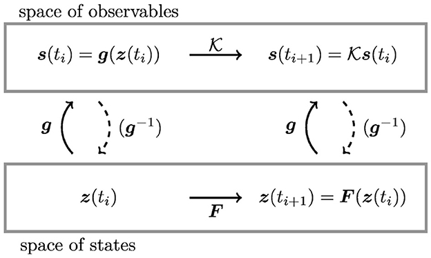
Figure 1. Illustration of Koopman operator theory. A finite, non-linear system described by states z∈ℝⁿ and a non-linear function F:ℝⁿ → ℝⁿ can be transformed into an often infinite-dimensional, linear system described by observables $s\in {ℝ}^{\mathcal{K}}$ and Koopman operator $\mathcal{K}:{ℝ}^{\mathcal{K}}\to {ℝ}^{\mathcal{K}}$. The measurement functions $g:{ℝ}^n\to {ℝ}^{\mathcal{K}}$ and their inverse counterparts $g^{-1}:{ℝ}^{\mathcal{K}}\to {ℝ}^n$ link between the two spaces.

For most systems, the Koopman operator is infinite-dimensional, as illustrated in [21], but in some cases, a finite-dimensional representation can be found, as an example in [6] shows. Essentially, the Koopman operator exists, if one can find a transformation of the non-linear system F into a linear one using the measurement functions g. The main challenge in Koopman operator theory is, thus, identifying a set of functions g for which the Koopman operator is finite [1, 21]. Many approaches to this challenge have been developed [2, 26], such as (Empirical) Dynamic Mode Decomposition (DMD) [17], Hankel-DMD [18], and the HAVOK-algorithm [1], which is the object of this study. If a finite-dimensional representation of the dynamical system at hand can be found, Koopman operator theory facilitates the identification of a global linear representation of the given non-linear system [1]. As the toolset and theoretical basis for linear system analysis are much larger and more robust, one would in many cases prefer a linear system description over a non-linear one. Even if an exact and finite-dimensional representation may not exist for a given system, the approximation of a finite-dimensional Koopman operator can still yield accurate system state-space models.

2.2. Time series similarity measures

Throughout this study, it is often necessary to estimate the accuracy of a model or an algorithm by comparing a ground truth time series x_true, typically the one measured, to the approximated time series x_approx, typically the one generated by HAVOK. To do so, the normalized mean absolute error is used, which is defined as

$\begin{array}{ll}\text{nMAE}=\frac{1}{l}{\displaystyle \sum _{t_i=1}^l}\frac{x_{\text{true}}(t_i)-x_{\text{approx}}(t_i)}{\text{max}(x_{\text{true}})},& (3)\end{array}$

where $x(t_i)\in {ℝ}^n$ is one uni-variate measurement within a time series x at time t_i. Each time series contains l different measurements at l different points t_i in time. This equation results in an error measure that is normalized to both the number of sampling points, i.e., the time series length, and the maximum amplitude of a time series. This choice is beneficial for measuring similarity across oscillatory time series of different lengths.

2.3. HAVOK and its parameters

After the basics of Koopman operator theory and the error measure have been explained, the HAVOK-algorithm [1] and its parameters will be described in the following. Figure 2 shows a flow chart of the HAVOK-algorithm, illustrating the six steps from data generation via the setup of the Hankel matrix, singular value decomposition, differentiation, sparse regression using the SINDy algorithm [6], to the compilation of the state-space system. The parameters of each individual step are marked on the left-hand side of the diagram.

FIGURE 2

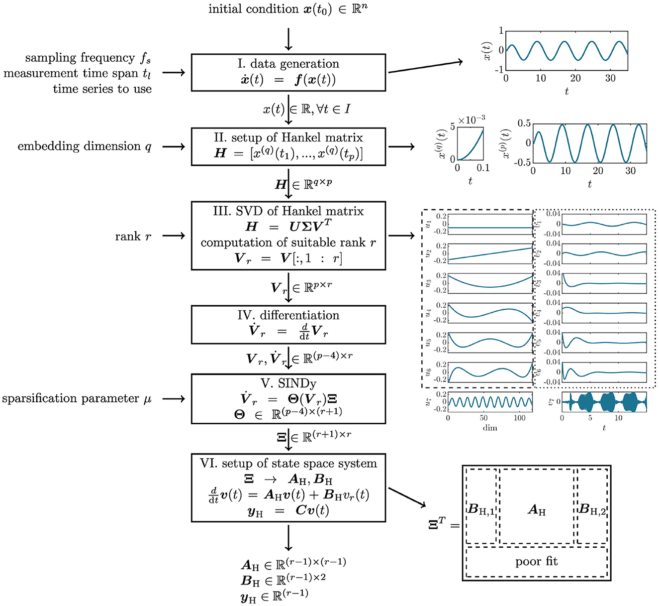
Figure 2. The six steps of the HAVOK algorithm, the parameters, and exemplary images of the data processed in each step. The vertical flow-chart illustrates the six steps data-generation, setup of the Hankel matrix, singular value decomposition (SVD) of the Hankel matrix, differentiation, sparse regression using the SINDy algorithm, and finally the setup of the state space system. On the left, the tuning parameters for each step are introduced. The images on the right-hand side of the figure illustrate the data each step is concerned with. From top to bottom. (1) The time series x(t) generated is the first step. (2) The time series sections x^(q)(t) and x^(p)(t) that form a column and a row of the Hankel matrix H, respectively. (3) The results of the SVD, represented by columns u_j and v_j of the matrices U and V. The u_j represents a coordinate system, while the v_j represents the evolution of these coordinates in time t. (4) The state space matrices A_H and B_H are setup by dividing up the matrix of sparse coefficients Ξ. The bottom row of Ξ is dropped as it represents a poor fit. Each step is described in detail in the respective section of the methods part of this study.

2.3.1. Data acquisition

The input to the HAVOK-algorithm is a one-dimensional time series x(t) of length t_l and sampled with frequency f_s. In theory, any measurement from a deterministic dynamical system could be used, as long as the dynamics are observable through that time series, as will be shown in detail later on. For the purpose of understanding the inner workings of the algorithm and its parameters, this study uses synthetic data generated through the integration of a known system of equations $\stackrel{•}{x}=f(x(t))$ in the first part, and measurement data from a real-world brake system in the second part. An exemplary time series is shown in the top right of Figure 2.

The data acquisition step has three parameters: the time series length t_l, the sampling frequency f_s, and the choice of degree of freedom from which the measurement is taken, although in practice, the latter two might be fixed by the sensor location. Naturally, those parameters will have an effect on the state-space model that is identified in the final step of the algorithm.

2.3.2. Time embedding

In a second step, the time series data x(t) is stacked with q time-shifted copies of itself into a Hankel matrix H∈ℝ^q×p, where the second dimension p is computed from the number of input samples l minus the embedding dimension q, such that p = l−q. Generally, the adaptive parameter of this step, i.e., the embedding dimension q is chosen such that q < < p. Figure 2 shows the resulting time series segments $x^{(q)}(t)\in ℝ,t\in \left[0,t_q\right],t_q>0$ and $x^{(p)}(t)\in ℝ,t\in \left[0,t_p\right],t_p>0$ which are contained in a column and a row of the Hankel matrix, respectively.

The procedure of using time-delayed observable as approximations of the Koopman operator was first introduced by Mezić and Banaszuk in [27] and is based on Takens' embedding theorem [28], which states that the state-space of a deterministic system can be uncovered from measurements in only one point. The relation of the Hankel matrix to the Koopman operator becomes apparent when rewriting the Hankel matrix H with the Koopman operator $\mathcal{K}$ to

$\begin{array}{ll}H=\left[\begin{array}{ccccc}x(t_1)& x(t_2)& x(t_3)& \mathrm{...}& x(t_p)\\ x(t_2)& x(t_3)& x(t_4)& \mathrm{...}& x(t_{p+1})\\ ⋮& ⋮& ⋮& \ddots & ⋮\\ x(t_q)& x(t_{q+1})& x(t_{q+2})& \mathrm{...}& x(t_l)\end{array}\right]=\left[\begin{array}{ccccc}x(t_1)& Kx(t_1)& K^{2}x(t_1)& \mathrm{...}& K^{p-1}x(t_1)\\ Kx(t_1)& K^{2}x(t_1)& K^{3}x(t_1)& \mathrm{...}& K^{p}x(t_1)\\ ⋮& ⋮& ⋮& \ddots & ⋮\\ K^{q-1}x(t_1)& K^{q}x(t_1)& K^{q+1}x(t_1)& \mathrm{...}& K^{l-1}x(t_1)\end{array}\right],& (4)\end{array}$

such that the states are propagated in time by the Koopman operator $\mathcal{K}$. Reordering the resulting matrix to

$\begin{array}{l}H=\left[\begin{array}{cccc}|& |& |& |\\ x^{(q)}(t)& K{x}^{(q)}(t)& \mathrm{...}& K^{p-1}{x}^{(q)}(t)\\ |& |& |& |\end{array}\right],\\ \text{where} x^{(q)}(t)=\left[\begin{array}{r}\hfill x(t_1)\\ \hfill Kx(t_1)\\ \hfill K^{2}x(t_1)\\ \hfill ⋮\\ \hfill K{x}^{q-1}x(t_1)\end{array}\right]=\left[\begin{array}{r}\hfill x(t_1)\\ \hfill x(t_2)\\ \hfill x(t_3)\\ \hfill ⋮\\ \hfill x(t_q)\end{array}\right]& (5)\end{array}$

shows that the matrix H consists of p time series sections x^(q)(t)∈ℝ, which could be interpreted as q-dimensional snapshots of the system. In the next step, a singular value decomposition is performed on the Hankel matrix in order to determine a q-dimensional function basis for these system snapshots.

2.3.3. Singular value decomposition

A singular value decomposition (SVD) is performed on the Hankel matrix H in the third step, which yields both a function basis for the snapshots x^(q)(t) and a description of the observed dynamics in the determined function space. The SVD decomposes the Hankel matrix H∈ℝ^q×p into three matrices

$\begin{array}{ll}H=U\Sigma V^T,& (6)\end{array}$

where U∈ℝ^q×q, Σ∈ℝ^q×p, and V∈ℝ^p×p. The orthonormal columns of the unit matrices U and V form a basis for the column- and row-space of the Hankel matrix H, respectively. The matrix Σ contains q so-called singular values σ_j on the main diagonal, which can be interpreted as representing the relative importance of the respective columns in U and V for representing the data in H. The singular values are ordered from largest to smallest, and, accordingly, the columns of U and V are ordered by their importance for representing the data in H. For a more detailed description of the SVD, see for example [21].

In the context of the HAVOK-algorithm, the columns $u_j\in {ℝ}^{q\times 1}$ of the matrix U form a basis for the column space of H and, thus, for the snapshots x^(q)(t), representing the Koopman observables $s(t_i)=g(x^{(q)}(t))$ as introduced in Figure 1. The vectors u_j provide a Koopman invariant subspace for the non-linear dynamics in the Hankel matrix. The time evolution of each u_j is described by the respective column $v_j\in {ℝ}^{p\times 1}$ of the matrix V. The vectors v_j can thus be interpreted as time series in the new coordinate system formed by the vectors u_j. Note that the transformation H = UΣV^T is unique up to simultaneously switching the signs of a column in U and V. Some exemplary observables u_j and new dynamics v_j are shown in Figure 2.

In [1], it was shown that only a small number of the columns of U and V are necessary to describe the dynamics of the different systems at hand. The model rank r, which also defines the size of the final state-space model, is determined from the singular values σ_j. Depending on the dynamical system at hand, the singular values may form an elbow curve, clearly separating more important columns from less important ones. In the original paper by Brunton et al. [1], the optimal rank r_{opt, GD} is computed by hard-thresholding the singular values with a method proposed in [29], where the threshold is computed as a function of the Hankel matrix dimensionality ratio q/p as

$\begin{array}{l}{\sigma }_{\text{thresh}}=(0.56{\left(\frac{q}{p}\right)}^3-0.95{\left(\frac{q}{p}\right)}^2+1.82\left(\frac{q}{p}\right)\\ +1.43{\sigma }_{\text{thresh}})·\text{median}({\sigma }_j).& (7)\end{array}$

However, it was found in the course of this study that this method often fails to locate the elbow in the curve, which is usually easy to determine visually. Figure 3 shows the singular values obtained with data from the double mass oscillator presented in Section 3.1. The rank r_{opt, GD} = 51 is located far away from the elbow. For the purpose of this study, the r_opt = 7, which is located at the elbow or kink of the curve, is used.

FIGURE 3

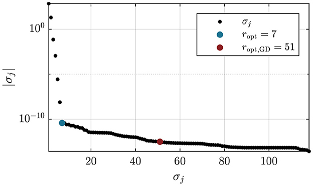
Figure 3. Determination of model rank r for the double mass oscillator system introduced in Section 3.1. The absolute values of the σ_j form an elbow curve. The method proposed in [1] yields the rank r_opt,GD = 51 which is much higher than the suitable model rank r_opt = 7 determined visually.

Implementing an elbow-finding algorithm such as the one proposed in [30] would help the automation of the HAVOK-algorithm at this point but is beyond the scope of this study. For the course of this study, the rank r for each system is chosen manually. Independent of which algorithm is chosen for the computation of the model rank, we recommend analyzing the singular values to confirm the choice of model rank for each new system.

With the obtained rank r, a matrix V_r = V[:, 1:r] is set up using the first r columns of V. The matrix $V_r\in {ℝ}^{p\times r}$ is a representation of the dynamics in the space of observables u_i and can be interpreted as an approximation of the Koopman operator in a Koopman-invariant subspace. In the remaining steps of the algorithm, a state-space system representing the dynamics in V_r is sought.

2.3.4. Time differentiation

In this step, the time derivative ${\stackrel{•}{V}}_r$ of the matrix V_r is computed, which is required for the computation of the linear system representation in the next step. As suggested in [1], a fourth-order central difference method

$\begin{array}{l}\dot{f}(x(t_i))=\frac{1}{12\Delta t}(f(x(t_i-2\Delta t))\\ -8f(x(t_i-\Delta t))+8f(x(t_i+\Delta t))-f(x(t_i+2\Delta t)))& (8)\end{array}$

is implemented, where $\Delta t=\frac{1}{f_S}$ denotes the time step size. The derivative ḟ(x(t_i)) of a state x(t_i) at time t_i is computed using two past and two future steps. The resulting matrix ${\stackrel{•}{V}}_r\in {ℝ}^{(p-4)\times r}$ is, thus, slightly reduced in dimension.

2.3.5. Sparse identification of non-linear dynamics

A sparse linear system representing the system dynamics contained in V_r is recovered using the matrix V_r and the matrix of derivatives ${\stackrel{•}{V}}_r$ using the sparse identification of non-linear dynamics (SINDy) algorithm, which was introduced by Brunton et al. in [6]. Sparse denotes a system description that comprises only a small number of terms compared to the space of ansatz functions used in the regression, thus yielding a very compact and simple set of differential equations. The SINDy algorithm is an equation-free method for obtaining differential equations describing the observed dynamics of a system from measurement data. First, a library of candidate functions $\Theta (V_r)\in {ℝ}^{(p-4)\times (r+1)}$ is set up from the matrix of measurements V_r, which for the HAVOK-algorithm is defined as

$\begin{array}{ll}\Theta (V_r)=\left[1V_r\right],& (9)\end{array}$

where 1∈ℝ^{(p−4) × 1} represents a bias matrix containing only entries of 1. SINDy will then identify the linear combination of those candidate functions that can represent the dynamics in V_r. As the goal of the HAVOK-algorithm is identifying a linear system, only linear terms are included here, even though the SINDy algorithm would allow for including non-linear terms in the function library, such as ${(v_{r,j})}^2$, where v_{r, j} denotes a column of the matrix V_r. With this function library and the state derivatives, a system of equations

$\begin{array}{ll}{\stackrel{•}{V}}_r=\Theta (V_r)\Xi & (10)\end{array}$

is set up. The matrix Ξ∈ℝ^{(r+1) × r} contains sparse vectors of coefficients ξ_j which are computed using a thresholded sequential least squares algorithm. The SINDy algorithm seeks to find a solution to this system of equations that minimizes the L¹-norm of the coefficients, promoting sparsity. Only a few terms in the coefficient vectors are non-zero for generating a sparse model ${\stackrel{•}{V}}_r=\Theta (V_r)\Xi$ with as less terms as possible. The sparsification knob μ, which is another important parameter of the HAVOK-algorithm, is introduced. After an initial least-squares guess $\Xi =\Theta {(V_r)}^{+}{\stackrel{•}{V}}_r$, all entries of Ξ smaller than μ are set to zero. The regression is performed again on the non-zero entries of Ξ, and once again, the resulting entries in Ξ are set to zero if their values are below the sparsification threshold μ. This process is repeated until it converges to a final sparse matrix Ξ, i.e., until no more small entries are set to zero within one iteration. The matrix Ξ now contains the few coefficients that govern the observed dynamics. With the final coefficients Ξ, it is possible to describe the system dynamics in the form of

$\begin{array}{ll}{\stackrel{•}{v}}_r={\Xi }^T{(\Theta (v_r^T))}^T,& (11)\end{array}$

where ${\stackrel{•}{v}}_r$ and v_r are no longer matrices containing time series measurement and their derivatives, but state vectors $v_r={\left[v_1,v_2,...,v_r\right]}^T$ forming the dynamical system described in state-space form.

The challenge in this step is to identify a Pareto-optimal μ that balances model accuracy, which is achieved with a smaller μ (deleting fewer terms), and model sparsity, which is implied by a larger μ (deleting more terms). In the original study, the authors propose increasing the sparsification threshold for each column, such that μ_j = jμ₀ and μ₀ = 0.02, while noting that μ = 0 yields better results, even though sparsity is not ensured in that case. In this study, an additional function is implemented to identify optimal sparsification parameters μ_j. Each column of the SINDy regression is considered separately. A set of 100 candidate sparsification thresholds μ∈[0.0001, 1] is tested. The SINDy algorithm is applied using each threshold, such that 100 different versions of a vector or sparse coefficients ξ_j are obtained. As a measure for model accuracy, the approximated derivative

$\begin{array}{ll}{\stackrel{•}{v}}_{\text{lin},j}={\xi }_j^T{(\Theta (V_r^T))}^T& (12)\end{array}$

is computed and compared to the original derivative v_{r, j}

$\begin{array}{ll}{\text{nMAE}}_j({\mu }_1)=\text{nMAE}({\stackrel{•}{v}}_{r,j}({\mu }_1),{\stackrel{•}{v}}_{\text{lin},j}({\mu }_1)),& (13)\end{array}$

using the normalized mean error. The result is a vector of normalized mean errors

$\begin{array}{ll}{\text{nMAE}}_{\mu ,j}=\left[{\text{nMAE}}_j({\mu }_1){\text{nMAE}}_j({\mu }_2)...{\text{nMAE}}_j({\mu }_{100})\right]\in {ℝ}^{1\times 100}.& (14)\end{array}$

As a measure for sparsity, the number of non-zero elements (NZE) in ξ_j normalized to the length r+1 of the vector is computed. By comparing these measures, nMAE for accuracy and NZE for sparsity, a suitable threshold value can be determined for each column of the sparsification. This procedure is repeated for each column separately, ultimately yielding a vector of threshold values μ_opt. The process would be rendered more exact by comparing the initial columns v_r with the HAVOK trajectories y_H instead of comparing the derivatives ${\stackrel{•}{v}}_{\mathrm{\text{lin}},j}$ and ${\stackrel{•}{v}}_{r,j}$ for the error measure, thus taking the interplay of the different columns into account. However, this expansion drastically increases the number of necessary computations and renders the numerical cost too high. Both the evolution of nMAE and NZE for one exemplary column are shown in Figure 4A. The smaller the sparsification parameter μ, the more terms are included, and the better the fit. On the other hand, if too few terms remain for large μ, the fit is not satisfying anymore. An optimal selection of μ will balance both competing quantities. For each column, an optimal sparsification parameter μ is obtained as the largest μ to yield an nMAE below a threshold value nMAE_thresh. This hard-thresholding of the nMAE results in an optimal μ_i for each column i that will satisfy that heuristic goodness of fit, see Figure 4B. As the magnitude of the nMAE is different for each dynamical system, it is necessary to adjust the sparsification threshold μ_thresh for each new system. We recommend studying the resulting nMAE for each column and choosing a threshold nMAE_thresh that is optimal for your individual purpose. A higher nMAE_thresh results in a larger μ and thus in a less accurate, but more sparse result, and vice versa.

FIGURE 4

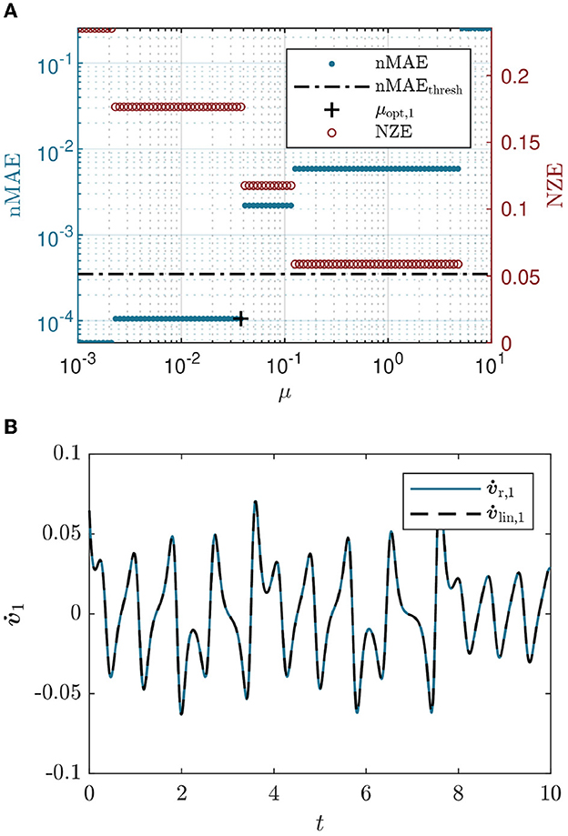
Figure 4. (A) Determination of an optimal sparsification threshold μ. The optimization is performed for each column of the sparse regression separately, the image shows the process for the first column only. The sparse regression is performed 100 times with different values of μ ∈ [0.0001,1] to obtain 100 different versions of a vector of sparse coefficients ξ_j. As a measure for accuracy, the nMAE of the resulting approximated derivative ${\stackrel{•}{v}}_{\text{lin},1}$ with its corresponding true derivative ${\stackrel{•}{v}}_{\text{r},1}$ is computed for each variation of μ. The relative number of non-zero elements (NZE) in the vector of sparse coefficients is a measure for model sparsity. By hard-threshold the nMAE at a value nMAE_thresh, a suitable μ for the given column is chosen. (B) Results of the sparse regression. The approximated derivative ${\stackrel{•}{v}}_{\text{lin},1}$ obtained with the indicated μ_{opt, 1} compared to the corresponding true derivative ${\stackrel{•}{v}}_{\text{r},1}$.

2.3.6. Construction of state-space representation

In the last step of the HAVOK-algorithm, a forced linear state-space system describing the system dynamics is set up from the matrix of sparse coefficients Ξ obtained through SINDy. To do so, the matrix Ξ^T is split into a state matrix $A_{\mathrm{\text{H}}}\in {ℝ}^{(r-1)\times (r-1)}$ and an input matrix $B_{\mathrm{\text{H}}}\in {ℝ}^{(r-1)\times 2}$ as illustrated in Figure 2. Precisely, the matrix B_H is set up from two sections of Ξ^T, B_{H, 1} and B_{H, 2}, each ∈ℝ^{(r−1) × 1}, such that B_H = [B_{H, 1}, B_{H, 2}]. The result is a forced state-space system representation in the form of

$\begin{array}{ll}\begin{array}{ll}\frac{\text{d}}{dt}v(t)\hfill & =A_{\text{H}}v(t)+B_{\text{H}}\left[\begin{array}{c}1\\ v_r(t)\end{array}\right]\hfill \\ y_{\text{H}}(t)\hfill & =Cv(t),\hfill \end{array}& (15)\end{array}$

with states v(t)∈ℝ^{(r−1) × 1} and a square r−1-dimensional identity matrix C. The output of the system is given by $y_{\mathrm{\text{H}}}\in {ℝ}^{(r-1)\times 1}$. The forcing v_r(t) is given by the last column of the matrix V_r. The forcing term is necessary for the reconstruction of the system dynamics when no closed-form representation of the Koopman operator can be found, i.e., to compensate for the approximation error. It was found by Champion et al. in [7], that a linear HAVOK model without forcing is sufficient to reconstruct the dynamics for quasi-periodic systems. For most cases, however, the forcing is necessary and the main drawback of this modeling approach as it is a priory only available for the time span t_l measured initially. There are different approaches to computing the forcing term beyond merely inserting the last column of V_r, including learning a forcing u^disc from the prediction error [31] and modeling the forcing using a second Hankel matrix [32].

The setup of the state-space system concludes the description of the HAVOK-algorithm and its parameters, specifically the sampling frequency f_s, measurement time span t_l, and chosen degree of freedom from the data acquisition step, the embedding dimension q, which is chosen during the setup of the Hankel matrix, the model rank r which has to be fixed after the SVD of the Hankel matrix, and the sparsification knob μ, which impacts the results of the sparse regression in the SINDy-step. Currently, the optimal selection, and the impact of a specific selection on the resulting model are unknown. In the previous paragraphs, possibilities for the computation of suitable values for these parameters have been introduced, sometimes beyond the original algorithm from [1]. In the next section, a deep dive into those parameters and how they influence each other will be taken.

2.4. Counter-intuitive action of embedding parameters

To illustrate the inner workings of the algorithm, several parameter studies have been performed that show how the parameters interact with each other and the final reduced-order model. In particular, some interrelations between parameters that are not obvious right away are pointed out here. These studies help to understand how the algorithm works and might thus help in choosing parameters for new systems.

First, it is important to note that the time spans contained in the rows and columns of the Hankel matrix, t_q and t_p, do not solely depend on the choice of the embedding dimension q, but also on the sampling frequency f_s. Essentially, more modes of vibration can be discovered if the sampling frequency is high. For a fixed embedding dimension q, a smaller sampling rate leads to less time series information in a column of the Hankel matrix H, while a larger sampling rate leads to a larger time span x^(q)(t). To cancel out the effect of the sampling frequency f_s on further results, it is prudent to define the time span in a column of H, x^(q)(t) instead of the embedding dimension q. For periodic motions, it is not necessary to use more than half a period of vibration in that column time span.

Second, the optimal rank r, i.e., the number of relevant modes u_i that results from the SVD, depends on the amount of information contained in x^(q)(t). If little information is contained in x^(q)(t), only a small number of basis functions are necessary to span the function space, but as the information in a column of H grows, so does the size of the space of basis functions, and thus the rank r. However, studies that were performed in the course of this study indicate that there is a maximum model rank r for a given system, which does not increase further even as x^(q)(t) is increased. These findings agree with assertions in the literature [31].

The combination of these two observations leads to the (at first counter-intuitive) observation that decreasing the sampling frequency f_s yields a larger number of relevant basis functions u_j and a larger model. This is because a larger sampling frequency f_s, together with a fixed embedding dimension q, results in a larger time span in x^(q)(t) and thus is a larger model rank r. If the time span x^(q)(t) is kept constant instead of the embedding dimension q when varying f_s, the obtained model rank r becomes independent of the sampling frequency f_s, up to a value when the sampling frequency becomes too coarse to accurately represent the core dynamics of the system. In realistic settings, the sampling frequency will be fixed, and a limited time series measurement will be available. Our recommendations for an optimal embedding process are given in Section 4.2.2.

3. Results

In this section, the results of the application of the HAVOK-algorithm to different mechanical oscillators are presented. Starting with a linear double-mass oscillator, the analytical model and the low-dimensional HAVOK model will be compared with a focus on which information of the analytical model can be extracted from the HAVOK model. Moving on, the dependence of the results on the algorithmic parameters is studied and the impact of varying model parameters such as initial conditions, damping, forcing type, and non-linearity is analyzed. These studies foster conclusions about which information of the true underlying dynamical system can be drawn from the data-driven reduced-order HAVOK model, and under which conditions this is possible. The exemplary application of HAVOK to real-world brake data, illustrating how parameters can be chosen for an unknown system, concludes this section.

3.1. Application to mechanical oscillators

The first step in the study of the application of HAVOK to mechanical oscillators is the double mass oscillator (DMO), which is shown in Figure 5. Two masses m_a and m_b are connected to each other and to the fixation points via spring-damper systems with linear spring constants k_j, j∈{1, 2, 3} and damping parameters d_j, j∈{1, 2, 3}. The displacement of the two masses in the horizontal direction is denoted by x_a and x_b, respectively. A forcing ψ, which in this first study is considered to be harmonic such that ψ(t) = Ψcos(Ωt) with amplitude Ψ and frequency Ω. Initially, the parameters are considered to be homogeneous, i.e., m_a = m_b = m, k₁ = k₂ = k₃ = k, and d₁ = d₂ = d₃ = d. The equations of motion for this system are given by

$\begin{array}{l}\underset{M_{\text{DMO}}}{\underbrace{\left[\begin{array}{cc}{m}_a& 0\\ 0& m_a\end{array}\right]}}\underset{{\ddot{x}}_{\text{DMO}}(t)}{\underbrace{\left[\begin{array}{c}{\ddot{x}}_a(t)\\ {\ddot{x}}_b(t)\end{array}\right]}}\\ +\underset{D_{\text{DMO}}}{\underbrace{\left[\begin{array}{cc}2d& -d\\ -d& 2d\end{array}\right]}}\underset{{\dot{x}}_{\text{DMO}}(t)}{\underbrace{\left[\begin{array}{c}{\dot{x}}_1(t)\\ {\dot{x}}_2(t)\end{array}\right]}}+\underset{K_{\text{DMO}}}{\underbrace{\left[\begin{array}{cc}2k& -k\\ -k& 2k\end{array}\right]}}\underset{x_{\text{DMO}}(t)}{\underbrace{\left[\begin{array}{c}{x}_1(t)\\ x_2(t)\end{array}\right]}}=\underset{{\psi }_{\text{DMO}}(t)}{\underbrace{\left[\begin{array}{c}\psi (t)\\ 0\end{array}\right]}},& (16)\end{array}$

FIGURE 5

Figure 5. The HAVOK model (bottom) for a double mass oscillator compared to its analytical basis (top). The state matrix A and input matrices B are shown in color code where red, white, and blue squares denote negative, zero, and positive entries of the matrices, respectively. To ensure that small values don't get lost in the color scale, all non-zero entries are marked with gray dots additionally. The eigenvalues of the two systems match. State-space representations and the time series comparisons show that the reduced-order model reproduces the dynamics of the original system well, except for a difference in amplitude, which is visible in the state space plots. For better visualization, the time series data of both x_a(t) and y_H,1(t) is normalized to have zero mean and a standard derivation of one.

where M_DMO is the mass matrix, D_DMO the damping matrix, and K_DMO the stiffness matrix. The states and their time derivatives are given by the vectors x_DMO, ẋ_DMO, and ẍ_DMO, respectively. The forcing vector is denoted by ψ_DMO. The damping is assumed to be in the form of Rayleigh damping, i.e., proportional to mass and spring stiffness

$\begin{array}{ll}{D}_{\text{DMO}}=\alpha M_{\text{DMO}}+\beta K_{\text{DMO}}& (17)\end{array}$

with stiffness- and mass-proportional damping parameters α and β. The system parameters are chosen such that the first damped eigenfrequency ω_{d, 1} = 1 rad/s and the mass m = 1 kg. The Lehr damping factors D_j [33] of the two eigenmodes of the DMO are 0 < D_j < 1, such that both modes are weakly damped. The forcing frequency is chosen to lie in between the damped eigenfrequencies such that ω_{d, 2} < Ω < ω_{d, 1}. The default parameters used with the DMO, the undamped eigenfrequencies ω_{0, j}, damped eigenfrequencies ω_{d, j}, and damping factors are listed in Table 1.

TABLE 1

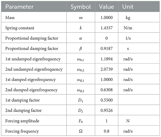
Table 1. Default parameters and resulting properties of the double mass oscillator.

The state-space model of the analytical DMO is set up as

$\begin{array}{ll}\begin{array}{ll}\underset{{\dot{x}}_{\text{DMO}}(t)}{\underbrace{\left[\begin{array}{c}{\dot{x}}_a(t)\\ {\dot{x}}_b(t)\\ {\ddot{x}}_a(t)\\ {\ddot{x}}_b(t)\end{array}\right]}}\hfill & =\underset{A_{\text{DMO}}}{\underbrace{\left[\begin{array}{rrrr}\hfill 0& \hfill 0& \hfill 1& \hfill 0\\ \hfill 0& \hfill 0& \hfill 0& \hfill 1\\ \hfill -\frac{2k}{m}& \hfill \frac{k}{m}& \hfill -\frac{2d}{m}& \hfill \frac{d}{m}\\ \hfill \frac{k}{m}& \hfill -\frac{2k}{m}& \hfill \frac{d}{m}& \hfill -\frac{2d}{m}\end{array}\right]}}\underset{x_{\text{DMO}}(t)}{\underbrace{\left[\begin{array}{c}{x}_a(t)\\ x_b(t)\\ {\dot{x}}_a(t)\\ {\dot{x}}_b(t)\end{array}\right]}}\hfill \\ +\underset{b_{\text{DMO}}}{\underbrace{\left[\begin{array}{c}0\\ 0\\ \frac{1}{m}\\ 0\end{array}\right]}}\underset{w_{\text{DMO}}(t)}{\underbrace{F_0\text{cos}(\Omega t)}}\hfill & \hfill \\ y_{\text{DMO}}(t)\hfill & =C_{\text{DMO}}{x}_{\text{DMO}}(t)\hfill \end{array}& (18)\end{array}$

where C_DMO is a 4 × 4 unitary matrix. Figure 5 shows a representation of the state matrix A_DMO and the input vector b_DMO in color-code: Red and blue squares mark negative and positive entries in the matrices, respectively. White squares denote zero entries, while gray dots mark all non-zero entries to ensure that no small entries are lost in the color scale. A state-space image of the dynamics of the system with $x_0={\left[0,0,0,0\right]}^T$ is also shown.

For this first study, the input to the HAVOK model is a time series of the x₁-coordinate, with an input time span t_l = 5T which is five times the forcing period $T=\frac{2\pi }{\Omega }$ and the sampling frequency f_s = 1 kHz. The parameters of the algorithm are set to the embedding dimension q = 118, the model rank r = 7, and the sparsification threshold $\text{nMA}{\text{E}}_{\mathrm{\text{thresh}}}=3.5·10^{-3}$, yielding a sparsification parameter μ = [0.0044, 0.0196, 0.2915, 0.0236, 0.3854, 1.0723, 0]^T. How changing those parameters affects the results will be studied in the next subsection. The resulting HAVOK model is shown in Figure 5, where the HAVOK state-space matrices A_H and B_H are depicted in the same color-code as previously, showing that the input matrix B_H is completely empty. The state matrix A_H has an almost block-diagonal shape, where the first two states are only connected to the rest of the states via two very small entries. The state-space formed by the first two states y_{H, 1} and y_{H, 2} of the HAVOK model resembles the state-space of the analytical model up to a scaling of the axes. The difference in scaling stems from the orthonormalization of the modes v_j during the SVD in the third step of the HAVOK algorithm, see Figure 2. The results from the SVD can be related to the input time series, both in terms of amplitude and dynamics, as the projection of the input time series onto a mode u_j fits the respective mode v_j multiplied with the singular value σ_j. Unfortunately, it is not as straightforward to regain this difference in amplitude for the final HAVOK model time series. Integrating a correction for this effect would be an interesting point for future research. The HAVOK eigenvalues match the true eigenvalues of the analytical model exactly, and an additional eigenvalue-pair on the imaginary axis matches the forcing frequency, as illustrated in Figure 5. For the linear DMO with harmonic forcing, the HAVOK-algorithm yields an unforced state-space model whose eigenvalues match the analytical eigenvalues exactly. This is an interesting finding, as we only observed a single degree of freedom, and did not specify the true dimensionality of the system, or any system parameters. Still, HAVOK is able to correctly identify the dynamic properties of the underlying system accurately (eigenvalues encode modal properties and stability).

3.1.1. Influence of HAVOK parameters

The results presented in the previous subsection are obtained with specific settings of parameters. In the following, the influence of the tuning parameters input time span t_l, input degree of freedom, model rank r, and sparsification parameter μ on the resulting HAVOK model and the information which can be extracted from it, are studied. These studies yield important insights into how to choose those parameters in order to determine a good low-rank representation of the dynamics. Figure 6A shows the results of varying each of these tuning parameters separately, which will be discussed in the following.

FIGURE 6

Figure 6. (A) HAVOK model results for variations of the algorithm parameters, studied by computing the model for a range of values. The state matrix A_H and HAVOK model eigenvalues for different input time spans t_l∈[T:10T]. In the figure, one column represents one matrix A_H, with the rows stacked on top of each other. This view allows for a direct comparison of the matrix entries. (B) HAVOK model results for variations of the algorithm parameters, studied by computing the model for a range of values. The state matrix A_H obtained when using different input time series x_a(t), x_b(t) or x_c(t) from the 3MO illustrated that the model rank can depend on the choice of input degree of freedom. (C) HAVOK model results for variations of the algorithm parameters, studied by computing the model for a range of values. HAVOK model matrices A_H and B_H obtained when varying only the model rank r∈[3:7], while using the x_a(t) time series of the DMO. It is shown that the magnitude of the matrix entries do not change when increasing rank. (D) The sparsification parameter μ and NZE for each column of the sparse regression when using the x_a(t) time series of the DMO and a model rank r = 7.

The measurement time length {t_l∈ρ·T|ρ∈ℕ, ρ ≤ 10} is varied in integer multiples of the forcing period. It controls the ratio of transient and steady state (periodic) motion that is contained in the input time span. The shorter the input time span, the larger the relative importance of the transient motion in the time series. Figure 6A shows the resulting state matrices A_H, and the respective eigenvalues for this variation. To visualize the variations of the matrix A_H, each matrix is represented as one column. For example, the left column in the Figure shows the matrix A_H for the first variant of t_l row-by-row. The evolution of each matrix entry for parameter variations becomes clearly visible since the corresponding entries lie directly next to each other. The input matrix B_H is not depicted as it remains all-zero over all variations. Only absolute values of the matrix entries are shown. It can be seen that as the input time span (and thus the relative importance of the periodic motion in the input time span) increases, the resulting state matrix becomes more sparse and for t_l>8T, HAVOK no longer correctly identifies the system eigenvalues. The forcing-related eigenvalues are identified correctly for all variations of the input time span.

To visualize the impact of the chosen measurement degree of freedom on the resulting system, a three-mass oscillator (3MO) is considered. We study each state as input to HAVOK separately. The three-mass oscillator model has the same structure as the DMO seen before, but with one additional mass. This dynamical system has three eigenmodes, where in the second eigenmode, only the two exterior masses at the two sides move. For the three depicted state matrices in Figure 6B, the input time series was taken to be the displacement of each of the masses x_a(t), x_b(t) and x_c(t). The dynamical system obtained with the two exterior measurements x_a(t) and x_c(t) has rank r = 8, while the middle degree of freedom x_b(t) results in a smaller r = 6 dimensional system. Analysis of the eigenvalues shows that while all models correctly contain the forcing frequency and the eigenvalues associated with the first and third eigenmodes, only the models obtained with x_a(t) and x_c(t) also contain the eigenvalue pair related to the second eigenmode, which is a physically consistent result with respect to the mode shapes.

The effect of varying the embedding dimension q, or time series section x^(q)(t), has already been discussed in a previous section, but the question of how to choose an optimal embedding dimension for a given measurement time series remains. Here, a large range of q was tested and the evolution of singular values σ_j and coordinates u_j was observed. Finally, an embedding dimension was chosen such that the coordinates u_j resemble Legendre polynomials, and the singular values yield a suiting rank value.

A study of the impact of the model rank of the system, where the model rank is varied such that {r∈ℕ|3 ≤ r ≤ 7} demonstrates that the chosen rank does not affect the magnitude of the values in the state-space matrix A or the input matrix. Instead, the non-zero part of the state matrix remains constant when increasing the rank, only adding values that were previously observed in the input matrix, see Figure 6C. Concerning the eigenvalues, it was found that the HAVOK model first contains the eigenvalue pair on the imaginary axis, which is related to the forcing frequency, and then adds the system-related, that is damped, eigenvalues.

The determination of the sparsification parameter has been described in a previous section. Figure 6D shows the chosen optimal sparsification parameter μ_opt for each column of the sparse regression along with the relative number of non-zero elements in the resulting matrix column. It shows that the sparsification parameter has an increasing trend with increasing column number and that its value is directly related to the sparsification process: For the last column, where μ₇ = 0, the column appears fully populated, as no sparsification takes place. Physically speaking, the dynamics contained in the last column are too complex to be matched by the simple linear ansatz space, even when fully populated. In the case of the linear oscillator with monochromatic forcing, the last column of the sparse regression does not contain physically meaningful information, it is simply a relic of the algorithm. However, for more general systems, e.g., when including non-linearities, this column contains the more complex dynamics which cannot be matched by the linear ansatz.

3.1.2. Dependence on physical model properties

After the dependence of the HAVOK results on the tuning parameters of the algorithm has been established, this section explores the evolution of the HAVOK model as the parameters of the analytical model itself change. The aim is to explore the limits of the HAVOK-algorithm as a method for obtaining low-order models that correctly represent the properties of the underlying system. The sensitivity of the HAVOK model for the double mass oscillator to changes in initial conditions, damping, and different forcing types is explored as well as the HAVOK model for non-linear double mass oscillators. The results are shown in Figures 7A, 9.

FIGURE 7

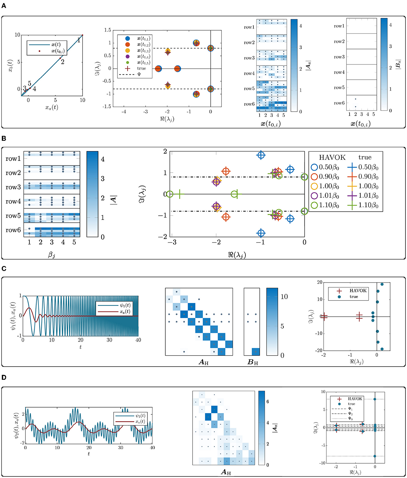
Figure 7. (A) Dependence of the HAVOK model on changes in the physical parameters of the analytical model. For each study, the double mass oscillator is used, varying one of the system parameters only. The HAVOK-DMO for different initial conditions along one trajectory result in different input time series. The resulting HAVOK model state and input matrices are show following the convention introduced in Figure 5. The respective model eigenvalues are compared to the forcing frequency and the eigenvalues of the underlying DMO system. (B) The HAVOK-DMO model for different damping values is illustrated by the state matrix. The all-zero input matrix is not represented. The eigenvalues for each model are shown in different colors, where circles represent the HAVOK model eigenvalues and crosses the true eigenvalues. One pair of HAVOK model eigenvalues lies on the imaginary axis for every model variation. (C) The application of HAVOK to a DMO forcing with a frequency-sweep type forcing shows entries on the sub-diagonal of the state matrix. In the representation of the eigenvalues, no forcing frequency is shown as it is varied continuously. (D) HAVOK-DMO model for a system that is forced with three superimposed sinusoids, where the HAVOK model catches both the system eigenvalues and the forcing frequency.

To study the dependency of the HAVOK model on the initial conditions, five exemplary initial conditions along one trajectory starting from $x(t_{0,1})={\left[10,10,0,0\right]}^T$ are chosen, where the first x(t_{0, 1}) is quite far away from the steady-state motion and the last x(t_{0, 5}) lies exactly on the steady-state, as shown in Figure 7A. The measurement time span t_l is kept constant while varying the initial conditions, such that the initial conditions further away yield an input time series with a larger fraction of transient motion. The resulting matrices and eigenvalues shown in Figure 7A illustrate that the state matrix becomes more sparse as the initial conditions approach the steady-state. While the forcing frequency and the first eigenvalue pair are always identified correctly, the second eigenvalue pair is not detected correctly for the time series with large transients, which originate from the initial conditions further away.

For the study of the damping parameter, the proportional damping factor β is varied such that β∈{0.5β₀, 0.9β₀, β₀, 1.01β₀, 1.1β₀}. A variation of the damping factor changes the damped eigenfrequencies of the system and with it the damping factors for both eigenmodes. With increasing β, the damped eigenfrequencies ω_d decrease, while the respective damping factor D increases. For β₅, the damping factor D₂>1, indicates that this mode becomes strongly damped. The second panel of Figure 7B shows the evolution of the state matrix A_H and the eigenvalues for the changes in the damping parameter. For all values of β, B_H is all-zero. The bottom rows of the state matrix change slightly, but the overall structure of the matrix remains the same. HAVOK correctly identifies all eigenvalues, except for the second eigenvalue pair for the strongest damping factor, which has been noted to correspond to a strongly damped mode.

Thus far, only harmonic monochromatic forcing has been considered. To analyze the influence of the forcing on the HAVOK model, two different cases are considered. First, a frequency-sweep forcing with ${\psi }_1(t)=\text{Ψ}\mathrm{\text{cos}}({\Omega }_0\frac{t}{2}t)$, where Ω₀ = 0.8 rad/s and second, a harmonic forcing with three superimposed frequencies given by ψ₂(t) = Ψ(cos(Ω₁t)+cos(Ω₂t)+cosΩ₃t)), with Ω₁ = 8 rad/s, Ω₂ = 0.8 rad/s and Ω₃ = 0.4 rad/s. The respective forcing and input time series are shown in Figures 7C, D along with the resulting HAVOK model matrices and eigenvalues. The HAVOK model for the system excited with three superimposed sinusoids is an unforced model with rank r = 11, and three eigenvalue pairs corresponding to the forcing frequencies on the imaginary axis. As before, HAVOK correctly identifies the eigenfrequencies of the system. The picture is very different for the frequency-forcing sweep excited model. Here, the structure of the resulting—now forced—state-space model of rank r = 10 is similar to the structure of the model that was identified for the chaotic Lorenz63 [34] system in the original [1] article. The HAVOK eigenvalues do not correspond to the system eigenvalues but include unstable eigenvalue pairs.

Non-linearity is introduced into the system by adding a cubic spring stiffness k_nl to the first spring k₁. The equations of motion are now given by

$\begin{array}{l}m{\ddot{x}}_a(t)+2d{\dot{x}}_a(t)-d{\dot{x}}_b(t)+2k{x}_a(t)-k{x}_b(t)-k_{\text{nl}}{x}_a^3(t)=\psi (t)\\ m{\ddot{x}}_b(t)-d{\dot{x}}_a(t)+2d{\dot{x}}_b(t)-k{x}_a(t)+2k{x}_b(t)=0& (19)\end{array}$

with a non-linearity $k_{\text{nl}}{x}_a^3$ in the first line. Two versions, a weakly non-linear model with k_{nl, 1} = 2k and a strongly non-linear model with k_{nl, 2} = 20k, are considered. The resulting HAVOK models are shown in Figure 8. Here, A_{H, lin}, A_{H, wnl}, and A_{H, snl} denote the system matrices of the linear, weakly non-linear, and strongly non-linear system, respectively. With a stronger non-linearity, the model rank increases, while the overall structure of the state matrix remains the same. As soon as a non-linearity is introduced, the HAVOK model becomes forced, i.e., B_H is no longer all-zero. At the same time, the non-linearity seems to keep the algorithm from correctly identifying the eigenvalues of the system. Instead, the HAVOK eigenvalues correspond to the forcing frequency and its higher-order harmonics, marked in the Figure by dotted lines.

FIGURE 8

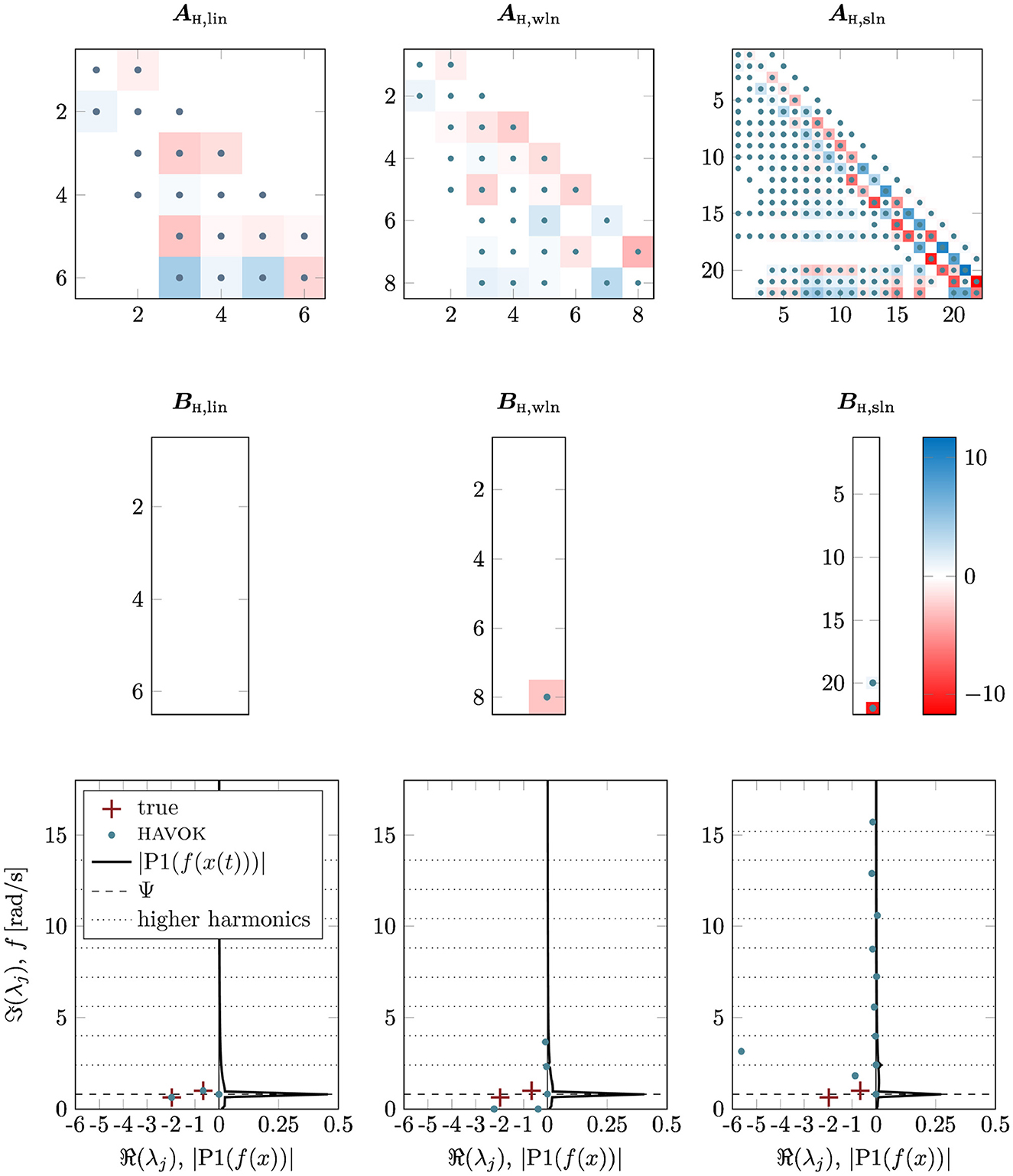
Figure 8. HAVOK models a linear, weakly non-linear, and strongly non-linear double mass oscillator. The state matrices A_H,lin, A_H,wnl, and A_H,snl are shown on top, with the input matrices B_H,lin, B_H,wnl, and B_H,snl below. The system eigenvalues λ_j of the true underlying DMO system, and the HAVOK model are shown on the bottom, along with a frequency spectrum of the input time series P1|f(x(t))|, the forcing frequency Ψ and its higher harmonics.

Two additional case studies with systems including non-linearity, the first neglecting all transient motion and the second moving the non-linearity to the spring k₃ on the other end of the oscillator chain, conclude the studies of parameter dependence. The resulting HAVOK models and their eigenvalues are both shown in Figure 9. The first two trajectories of the HAVOK model are shown as y_{H, wnl, 1}(t) and y_{H, wnl, 2}(t). The HAVOK model obtained from only the steady-state oscillation of the non-linear oscillator has a dominant off-diagonal structure, where the states as strongly coupled pair-wise. Its eigenvalues correspond to the forcing frequency and its higher harmonics on the imaginary axis, there is no signature of the linearized system's eigenvalues. For the model with the non-linearity away from the excitation and the measurement time series, the structure of the state matrix resembles the structure of previous state matrices, i.e., is less dominated by the diagonal. The eigenvalues of this system correspond closely to the eigenvalues of the analytical model, the forcing frequency, and one higher-order harmonic. Both these HAVOK models are forced, the same as the previous non-linear models.

FIGURE 9

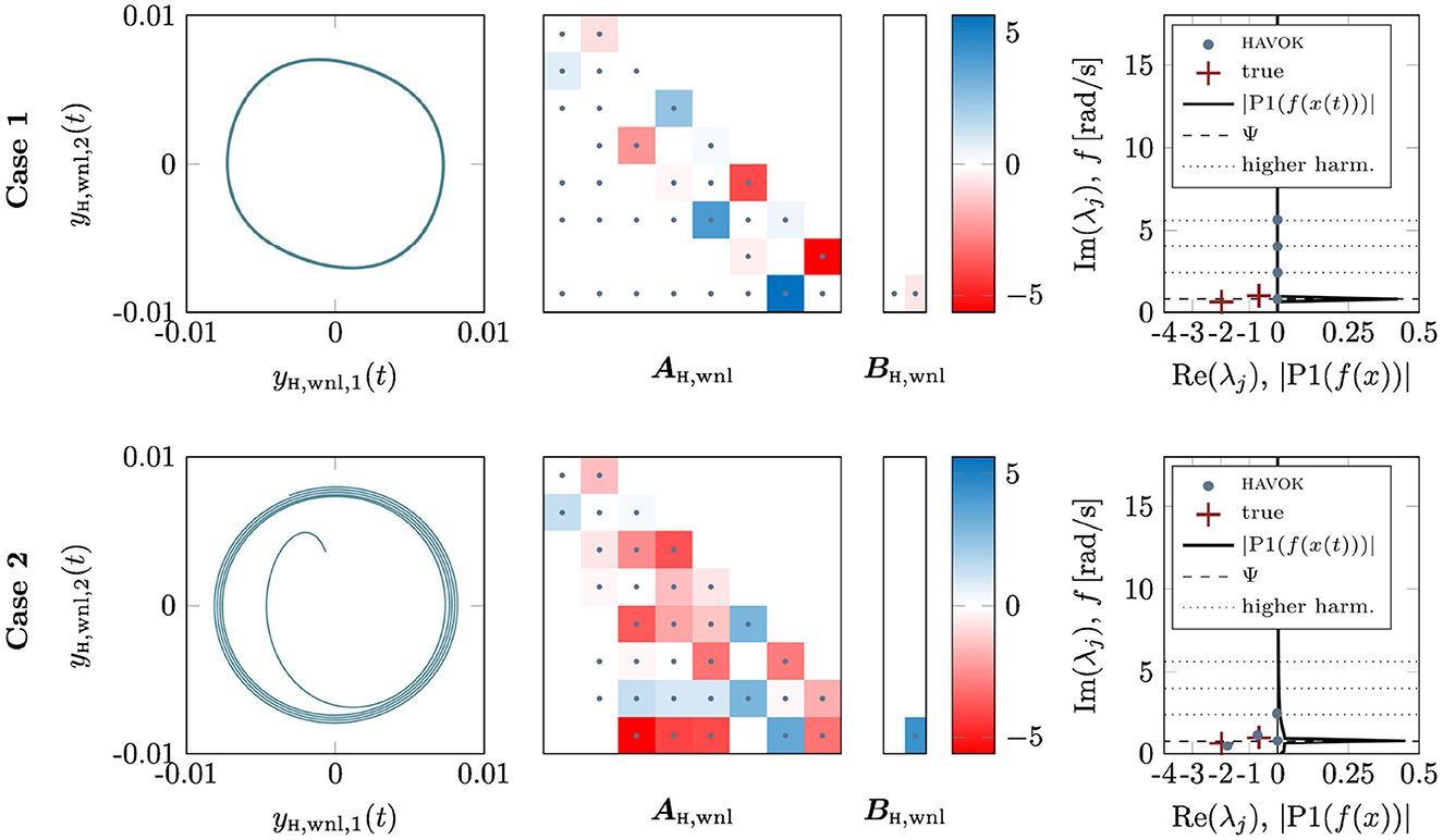
Figure 9. Case studies of the weakly non-linear double-mass-oscillator. (Top) The HAVOK model obtained when omitting all transient motion in the input time series. (Bottom) The HAVOK model for a DMO when the non-linearity is moved to the other end of the oscillator chain, away from the excitation and the input time series. For both systems, the state space resulting from the first two HAVOK trajectories y_H,wnl,1 and y_H,wnl,2 are shown, as well as the state and input matrices. On the right, the HAVOK model eigenvalues are compared to the true DMO system eigenvalues, the frequency spectrum P1|f(x)| of the input time series and the forcing frequency.

3.2. Application to a real-world brake system

Thus far, the low-order HAVOK models obtained from synthetic data have been considered, which enabled the comparison of the true analytical model (generating the data) and the HAVOK model. To round off this study, HAVOK is applied to real-world measurement data obtained with a microphone during the actuation of a friction disc brake system of a passenger car. For details regarding the experimental setup, see [35] and [36]. Friction brakes can exhibit squeal noises during braking, resulting from complex self-excited machine dynamics whose mechanisms have not yet been fully understood today [35]. There are two different prominent theories as to the process that yields brake squeal. Both of these theories are based on studying the silent (not squealing) and the squealing section of a brake stop separately and agree on a regime shift between the two dynamical states, which leads to qualitatively different dynamics in the two regimes. One theory states that the squealing, which is represented by a low-dimensional attractor, originates from the equilibrium-point dynamics in the non-squealing regime losing its stability [37], for example through a Hopf bifurcation. The other theory identifies 8–12-dimensional attractors in the silent regime, which transition toward a lower-dimensional attractor of 3–6 dimensions in the squealing regime [35, 38, 39]. These studies all agree on signs of chaotic dynamics in both the silent and the squealing regimes. As the realistic brake system is comprised of multiple components, actuation and a complex friction interface, the identification of a reduced order model using only measurement data is highly interesting, also to study the aforementioned root causes of the vibrations.

The microphone data was sampled at 51.2 kHz and bandpass-filtered with cutoff frequencies at 1 and 20 kHz. Two exemplary samples are taken from a single brake stop that is not squealing in the beginning and then exhibiting strong squeal events toward the end. To obtain a sufficient quality of the numerical derivatives during the application of HAVOK, it is necessary to upsample the data to 5,120 kHz for the silent and 512 kHz for the squealing region. The upsampling was performed using a Matlab spline interpolation function. The entire microphone signal and the two exemplary snippets are shown in Figure 10. Characteristic differences are visible in both time series.

FIGURE 10

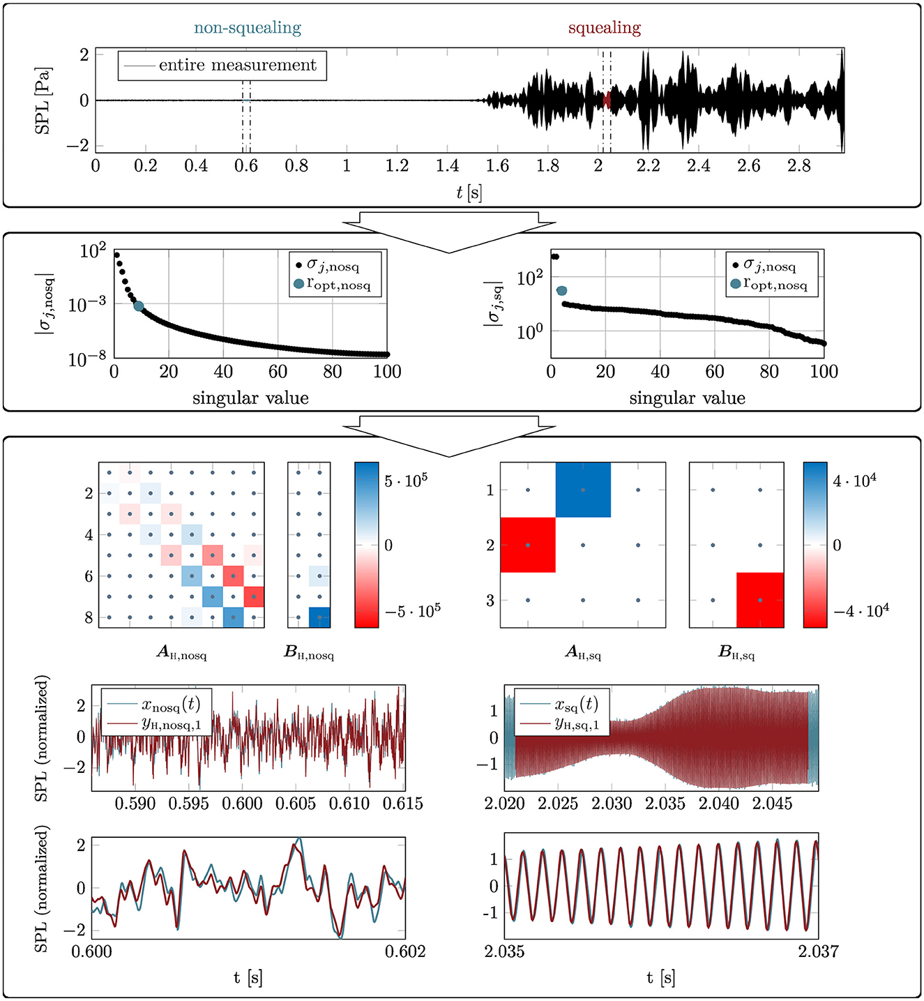
Figure 10. Application of the HAVOK algorithm to real-world measurement data. The sound pressure level (SPL) obtained with a microphone during the actuation of the friction brake of a passenger car is shown on the top. The dash-dotted lines indicate the sections from the silent and squealing regime used as input to the HAVOK algorithm. The singular values for each regime are visible in the center panel. In the bottom panel, the HAVOK model state matrices A_H and the input matrices B_H are shown, along with the resulting time series y_H,1(t) compared to the input time series x(t). As before, both time series are normalized to have zero mean and a standard derivation of 1.

The tuning parameters of the HAVOK algorithm are chosen as follows. For the input data, only the chosen time span t_l remains a flexible parameter, as the sampling frequency is fixed. Section lengths of 150,000 samples and 15,000 samples are taken from the silent and the squeal region, respectively, resulting in t_l≈0.03 s for both regimes. This time length was shown to yield consistent results with time delay embedding in [35]. As has been explained in the previous sections, the embedding dimension q and the model rank r are closely related, as the model rank is obtained from the results of the SVD, which depend on the embedding dimension q. To find an optimal embedding dimension and rank, the embedding dimension is initially set to q = 100 and varied over a large value range. The optimal values are determined based on the ability of the final HAVOK model to represent the measured dynamics, computed as the fit between the measurement data and the trajectory of the first HAVOK state y_{H, 1}(t). For the silent section, q = 100 and r = 9 are found, and q = 1, 000 and r = 4 for the squealing section. Note that the time span x^(q)(t) in a column of the Hankel matrix H is very different between the two regimes due to the different embedding dimensions. Figure 10 shows the first 100 singular values for each section which lead to the choice of model rank. For the squealing regime on the right, the choice of rank is obvious through the elbow-like formed curve. For the silent region, no clear kink in the curve is visible, making the choice of rank more heuristic. The sparsification parameter μ is set to zero for this initial study because the computational cost of obtaining an optimal μ is very high and was beyond the scope of this study. Due to this setting, no sparsification takes place in the SINDy regression, but a dominant structure of the state matrices is still clearly visible, see Figure 10. In the original study by Brunton et al. [1], where the algorithm was first introduced, the sparsification parameter μ was often kept at zero, too.

For both regimes, the HAVOK model reproduces the measured dynamics well except for a difference in amplitude which has been elaborated on in Section 3.1. Figure 10 shows the state matrix A_H and the input matrix B_H of the low-order HAVOK model as well as the attractors build from the first three states y_{H, 1}(t), y_{H, 2}(t) and y_{H, 3}(t) for the silent and squealing region, respectively. Both models are forced and a dominant structure with only a few large coefficients is visible in the matrices. The state matrix A_{H, nosq} of the silent section exhibits a clear structure with dominant entries on the two sub-diagonals. This matrix structure resembles that of the HAVOK model for the chaotic Lorenz attractor presented in [1]. The much smaller model of the squealing section shows two states are strongly coupled, and a third is mainly driven by the forcing term. The resulting attractors are shown as black lines, where the forcing is small, and red lines, where the forcing is larger. In the silent regime, no clear structure of the attractor or forcing patterns is discernible. In the squealing regime, the dynamics form concentric circles around the y_{H, 3}-axis, being tilted slightly with respect to the (y_{H, 1}, y_{H, 2})-plane. The forcing marks the transitions of the system from one radius to another.

4. Discussion

The results presented in the previous section show that the HAVOK algorithm can be used to obtain low-order state-space models that are able to reproduce the dynamics of the measured system well. The studies with the double mass oscillator reveal that the amount of system properties that can be extracted from the HAVOK state-space model depends on the type of underlying dynamical process, as will be discussed in detail in Section 4.1. Extensive studies of the effects of the HAVOK parameters on the resulting HAVOK model and the inner workings of the algorithm give rise to recommendations for choosing these parameters when applying HAVOK to a new model, as will be elaborated on in Section 4.2.

It has been shown how HAVOK can be applied to real-world measurement data where the type of underlying dynamics are still subject to discussion. Even for the complex dynamical system at hand, HAVOK is able to generate a model that reproduced the dynamics well. It becomes clear that the obtained model ranks for the silent r = 9 and squealing r = 4 section agree well with the theories presented in the literature. At the same time, the HAVOK models do not allow for much further information, for example on the damping properties of the system. Taking a step back and considering the results of the studies of the double and three-mass oscillators, these results are not surprising.

4.1. Physical interpretability

The fundamental research question for the study at hand is: how much information can one obtain from a fully data-driven system identification process using HAVOK, and how can the resulting system description be linked with classical physics-based descriptions? For all of the considered models, the HAVOK algorithm generates state-space systems that are able to reproduce the observed dynamics well. The reconstructed state space trajectories y_{H, j} of the HAVOK model will most likely be distorted compared to the original one due to the orthonormalization that takes place during the SVD. Whether or not it is possible to accurately recover the original amplitude from the process remains subject to further studies.

HAVOK builds up a state-space system based on the frequency components in the input time series. Therefore, a closed-form representation of the Koopman operator, i.e., an unforced state-space system, is found for a dynamical system with a finite number of frequency components, such as the linear double mass oscillator with harmonic forcing. For this special type of system, the HAVOK model accurately captures the true eigenvalues and thus some of the properties of the original system. The dependency on the periodicity of the input signal is also emphasized by the fact that periodic dynamics can be represented by a more sparse model, as the studies with different initial conditions and input time series lengths illustrate. It has also been shown that the rank of the HAVOK model depends directly on the number of frequency components in the input data. Note that even though HAVOK captures the dynamics and the eigenvalues for dynamics with a finite number of frequency components, it cannot distinguish between system-inherent and forcing-related contributions in the data. Therefore, HAVOK yields an unforced state space model whenever possible, as no distinction between the different components is possible without additional information on the underlying system.

For general systems that include non-linearities or non-harmonic forcing, no closed-form representation of the Koopman operator can be found and the resulting HAVOK model is forced, as is to be expected. The forcing will collect all dynamics that cannot be represented by the linear Koopman operator. In these cases, a lot of information on the underlying dynamical system is moved into the forcing term of the HAVOK model and is not accessible for further analysis in the state matrix A_H. Some information on the dimensionality, stability, and main spectral components of the underlying dynamical system can still be found, but the extraction of principles, coupling between the states, or generalizations, remains difficult.

As with any data-driven method, the system identification potential of the HAVOK algorithm is limited by the fact that only observable dynamics can be represented in the final model, as the study with the three-mass oscillator showed. Measurements from a degree of freedom that does not move with a specific mode cannot be used to create a model that represents that mode. The same is true for strongly damped modes that do not affect enough oscillations to become visible in the measurement data and are thus not present in the HAVOK model.

4.2. Recommendations for choosing HAVOK parameters

From the numerous studies of the HAVOK algorithm with different mechanical oscillator models, we derive some recommendations for choosing suitable parameter settings in order to obtain the most meaningful HAVOK model possible.

4.2.1. Input data

The input data forms the basis for the HAVOK model and may be subject to several parameter choices during the first step of the algorithm. First, if a choice of potential input data is available, choose a time series x(t) that contains rich information on the underlying dynamics and captures as many different modes as possible in order to get a more complete picture of the dynamics at hand. The sampling frequency f_s has to be high enough to represent the dynamics in the desired time scale. It is recommended to check the accuracy of the derivatives ${\stackrel{•}{V}}_r$ in the fourth step of the algorithm by reintegrating the obtained derivatives and comparing them to the original modes V_r. If the differentiation error is larger than 1% nMAE, the input signal x(t) should be upsampled using a suitable algorithm, until sufficient differentiation accuracy can be assured. The input time span t_l chosen from the measurement data is an important parameter that impacts the final HAVOK model. If the possibility of capturing both transient and steady-state dynamics is given, a mixture of both regimes was shown to yield robust and consistent results. Omitting the transient part completely prevents HAVOK from correctly capturing the system-related part of the dynamics (particularly damping), while large transients with strongly dissipative dynamics lead to an overestimation of the damping factors by the HAVOK algorithm. On the other hand, it seems that only transient motion, as in the case study with the frequency sweep function or the self-excited friction brake system, HAVOK cannot pick up the properties of the dynamical system itself in a fashion that is directly extractable, though it still yields a good reconstruction of the underlying dynamics and, in some cases, of the dimensionality of the system.

4.2.2. Embedding dimension and model rank

The embedding dimension q defines the amount of information that is contained in one column of the Hankel matrix H which is set up in the second step of the algorithm. The model rank r, which is chosen in the third step after the SVD of the Hankel matrix, marks the number of columns of the matrix V which are taken along for the sparse regression and ultimately defines the rank of the final model. Because the model rank r is generally chosen as the number of relevant components that are computed in the singular value decomposition, these two tuning parameters are closely connected. There are two approaches to deciding on an embedding dimension and model rank.

If the information on the desired model rank is available, either from prior knowledge of the system or from a fixed, desired output model rank, then the embedding dimension q can simply be varied until the singular value decomposition yields the desired number of relevant components. A larger embedding dimension q or, more accurately, a larger time span x^(q)(t), yields more valid coordinates and thus a higher model rank r, while a smaller value of q yields a smaller rank r. A good initial guess for the model rank r is the number of frequency components of the model and its forcing times two.

If no specific model rank r can be expected or is desired, it is recommended to vary the embedding dimension q over a wide value range and observe how the resulting model rank evolves. A model rank can then be chosen as a larger value, if a high model accuracy is desired, or a smaller value if a low-order model is wanted.

For the models studied in the course of this study, a variation of embedding dimension in the range of q∈[50:1, 000] was found to be sufficient. For periodic or quasi-periodic systems, a good starting point is an embedding dimension that yields a time span x^(q)(t) = (q−1)Δt that matches one period of the system [7]. For any system, the embedding dimension has to capture enough of the oscillation. If q is too small, the Koopman observables or u_j obtained from the SVD are highly non-linear and do not form a good basis for the HAVOK model [7]. According to Dylewsky et al. in [31], the embedding dimension q can be too small, but not too large. Our studies showed that there is an upper limit to the model rank r that can be obtained for a given system through variation of embedding dimension, above which no reasonable results are achieved.

4.2.3. Sparsification threshold

The sparsification threshold μ is set to define the cutoff threshold for small coefficient entries in the sparse identification of non-linear dynamics in the fifth step of the HAVOK algorithm. The parameter does not impact the dominant structure of the resulting state matrices but induces the final state and input matrices A_H and B_H to be more sparse. Finding a Pareto-optimal μ between model sparsity and model accuracy requires large computational efforts when performed extensively. It is possible to compute the vectors of sparse coefficients for a range of sparsification thresholds and compare the resulting non-zero elements and model accuracy for each individual state [3], as presented in Section 2.3.5. From this, an optimal sparsification threshold for each state can be found. However, since the dominant structure is not affected by the sparsification, it may be sufficient to set the sparsification threshold μ = 0.

5. Conclusion

In this study, the steps of the HAVOK algorithm, its parameters, their interconnections, and the relation of the method to the Koopman operator theory have been presented. The studies were performed in Matlab. Several mechanical oscillator models, ranging from linear to non-linear, weakly to strongly damped, excited with different types of forces, and subjected to different initial conditions, have been subjected to the HAVOK algorithm. The resulting low-order HAVOK state-space models have been compared to the analytical physics-based models to determine which properties of the underlying dynamical systems can be extracted from the data-driven approach and under which conditions. For all of the considered systems, the obtained HAVOK models reproduce the measured dynamics well. Information on the underlying (i.e., the data-generating) system dimensionality, stability, and dominant frequency components can be obtained in most cases, but detailed information such as eigenvalues can only be identified correctly for systems with a low number of frequency components in our study. The HAVOK algorithm is, thus, a good choice if a low-order model is required for future state prediction or control purposes of a complex and unknown dynamical process. However, the method is of limited use as a system identification algorithm when system properties are to be identified in the classical sense of modal properties. Extensive studies of the effects of the algorithm's parameters yield valuable insights into the inner workings of the algorithm and give rise to recommendations for choosing those parameters when applying the method to new systems.

Data availability statement

The raw data supporting the conclusions of this article will be made available upon reasonable request.

Author contributions

MS and CG contributed to the conception and design of the study. CG performed the analysis and investigation and wrote the first draft of the manuscript. MS supervised the study. All authors contributed to the manuscript revision, have read, and approved the submitted version.

Funding

This research was funded by the German Research Foundation (Deutsche Forschungsgemeinschaft DFG) within the Priority Program 1897 calm, smooth, smart, grant number 314996260.

Conflict of interest

The authors declare that the research was conducted in the absence of any commercial or financial relationships that could be construed as a potential conflict of interest.

Publisher's note

All claims expressed in this article are solely those of the authors and do not necessarily represent those of their affiliated organizations, or those of the publisher, the editors and the reviewers. Any product that may be evaluated in this article, or claim that may be made by its manufacturer, is not guaranteed or endorsed by the publisher.

References

1. Brunton SL, Brunton BW, Proctor JL, Kaiser E, Kutz JN. Chaos as an intermittently forced linear system. Nat Commun. (2017) 8:19. doi: 10.1038/s41467-017-00030-8

PubMed Abstract | CrossRef Full Text | Google Scholar

2. Mezić I. Koopman operator, geometry, and learning of dynamical systems. Not Am Math Soc. (2021) 68:1087–105. doi: 10.1090/noti2306

PubMed Abstract | CrossRef Full Text | Google Scholar

3. Stender M, Oberst S, Hoffmann N. Recovery of differential equations from impulse response time series data for model identification and feature extraction. Vibration. (2019) 2:25–46. doi: 10.3390/vibration2010002

CrossRef Full Text | Google Scholar

4. Conti P, Gobat G, Fresca S, Manzoni A, Frangi A. Reduced order modeling of parametrized systems through autoencoders and SINDy approach: continuation of periodic solutions. Comput Methods Appl Mech Eng. (2023) 411:116072. doi: 10.1016/j.cma.2023.116072

Crossref Full Text | Google Scholar

5. Guckenheimer J, Holmes P. Global bifurcations. In: Nonlinear Oscillations, Dynamical Systems, and Bifurcations of Vector Fields (New York, NY: Springer) (1983). p. 289–352.

Google Scholar

6. Brunton SL, Proctor JL, Kutz JN. Discovering governing equations from data by sparse identification of nonlinear dynamical systems. Proc Natl Acad Sci USA. (2016) 113:3932–7. doi: 10.1073/pnas.1517384113

PubMed Abstract | CrossRef Full Text | Google Scholar

7. Champion KP, Brunton SL, Kutz JN. Discovery of nonlinear multiscale systems: sampling strategies and embeddings. SIAM J Appl Dyn Syst. (2019) 18:312–33. doi: 10.1137/18M1188227

CrossRef Full Text | Google Scholar

8. Bakarji J, Champion K, Kutz JN, Brunton SL. Discovering governing equations from partial measurements with deep delay autoencoders. arXiv. (2022). doi: 10.48550/arXiv.2201.05136

CrossRef Full Text | Google Scholar

9. Franco N, Manzoni A, Zunino P. A deep learning approach to reduced order modelling of parameter dependent partial differential equations. Math Comp. (2023) 92:483–524. doi: 10.1090/mcom/3781

PubMed Abstract | CrossRef Full Text | Google Scholar

10. Fresca S, Manzoni A. POD-DL-ROM enhancing deep learning-based reduced order models for nonlinear parametrized PDEs by proper orthogonal decomposition. Comput Methods Appl Mech Eng. (2022) 388:114181. doi: 10.1016/j.cma.2021.114181

PubMed Abstract | CrossRef Full Text | Google Scholar

11. Daniels BC, Nemenman I. Automated adaptive inference of phenomenological dynamical models. Nat Commun. (2015) 6:8133. doi: 10.1038/ncomms9133

PubMed Abstract | CrossRef Full Text | Google Scholar

12. Atkinson S. Bayesian hidden physics models: uncertainty quantification for discovery of nonlinear partial differential operators from data. arXiv. (2020). doi: 10.48550/arXiv.2006.04228

CrossRef Full Text | Google Scholar

13. Ribera H, Shirman S, Nguyen A, Mangan N. Model selection of chaotic systems from data with hidden variables using sparse data assimilation. Chaos. (2022) 32:063101. doi: 10.1063/5.0066066

PubMed Abstract | CrossRef Full Text | Google Scholar

14. Schmidt M, Lipson H. Distilling free-form natural laws from experimental data. Science. (2009) 324:81–5. doi: 10.1126/science.1165893

PubMed Abstract | CrossRef Full Text | Google Scholar

15. Schmid PJ. Dynamic mode decomposition of numerical and experimental data. J Fluid Mech. (2010) 656:5–28. doi: 10.1017/S0022112010001217

CrossRef Full Text | Google Scholar

16. Rowley CW, Mezić I, Bagheri S, Schlatter P, Henningson DS. Spectral analysis of nonlinear flows. J Fluid Mech. (2009) 641:115–27. doi: 10.1017/S0022112009992059

CrossRef Full Text | Google Scholar

17. Williams MO, Kevrekidis IG, Rowley CW. A data-driven approximation of the Koopman operator: extending dynamic mode decomposition. J Nonlinear Sci. (2015) 25:1307–46. doi: 10.1007/s00332-015-9258-5

CrossRef Full Text | Google Scholar

18. Arbabi H, Mezić I. Ergodic theory, dynamic mode decomposition, and computation of spectral properties of the Koopman operator. SIAM J Appl Dyn Syst. (2017) 16:2096–126. doi: 10.1137/17M1125236

CrossRef Full Text | Google Scholar

19. Somacal A, Barrera Y, Boechi L, Jonckheere M, Lefieux V, Picard D, et al. Uncovering differential equations from data with hidden variables. Phys Rev E. (2022) 105:054209. doi: 10.1103/PhysRevE.105.054209

PubMed Abstract | CrossRef Full Text | Google Scholar

20. Champion K, Lusch B, Kutz JN, Brunton SL. Data-driven discovery of coordinates and governing equations. Proc Nat Acad Sci USA. (2019) 116:22445–51. doi: 10.1073/pnas.1906995116

PubMed Abstract | CrossRef Full Text | Google Scholar

21. Brunton SL, Kutz JN. Data-Driven Science and Engineering: Machine Learning, Dynamical Systems, and Control. Cambridge: Cambridge University Press (2019).

Google Scholar

22. Mezić I. Analysis of fluid flows via spectral properties of the Koopman operator. Annu Rev Fluid Mech. (2013) 45:357–78. doi: 10.1146/annurev-fluid-011212-140652

CrossRef Full Text | Google Scholar

23. Lusch B, Kutz JN, Brunton SL. Deep learning for universal linear embeddings of nonlinear dynamics. Nat Commun. (2018) 9:4950. doi: 10.1038/s41467-018-07210-0

PubMed Abstract | CrossRef Full Text | Google Scholar

24. Koopman BO. Hamiltonian systems and transformation in Hilbert space. Proc Natl Acad Sci USA. (1931) 17:315–8. doi: 10.1073/pnas.17.5.315

PubMed Abstract | CrossRef Full Text | Google Scholar

25. Mezić I. Spectral properties of dynamical systems, model reduction and decompositions. Nonlinear Dyn. (2005) 41:309–25. doi: 10.1007/s11071-005-2824-x

CrossRef Full Text | Google Scholar

26. Parmar N, Refai H, Runolfsson T. A survey on the methods and results of data-driven Koopman analysis in the visualization of dynamical systems. IEEE Transact Big Data. (2020) 8:1. doi: 10.1109/TBDATA.2020.2980849

CrossRef Full Text | Google Scholar

27. Mezić I, Banaszuk A. Comparison of systems with complex behavior: spectral methods. In: Proceedings of the 39th IEEE Conference on Decision and Control (Cat No00CH37187) (Sydney). (2000) p. 1224–31.

Google Scholar

28. Takens F. Detecting strange attractors in turbulence. In: Dynamical Systems and Turbulence, Warwick 1980, Vol 898 (Berlin: Springer). (1981). p. 366–81. doi: 10.1007/BFb0091924

PubMed Abstract | CrossRef Full Text | Google Scholar

29. Gavish M, Donoho DL. The optimal hard threshold for singular values is 4/sqrt(3). IEEE Transact Inf Theory. (2014) 60:5040–53. doi: 10.1109/TIT.2014.2323359

CrossRef Full Text | Google Scholar

30. Branke J, Deb K, Dierolf H, Osswald M. Finding knees in multi-objective Optimization. In: International Conference on Parallel Problem Solving From Nature (Birmingham). (2004) p. 722–31.

Google Scholar

31. Dylewsky D, Kaiser E, Brunton SL, Kutz JN. Principal component trajectories for modeling spectrally continuous dynamics as forced linear systems. Phys RevE. (2022) 105:015312. doi: 10.1103/PhysRevE.105.015312

PubMed Abstract | CrossRef Full Text | Google Scholar

32. Khodkar MA, Hassanzadeh P, Antoulas A. A Koopman-based framework for forecasting the spatiotemporal evolution of chaotic dynamics with nonlinearities modeled as exogenous forcings. arXiv. (2019). doi: 10.48550/arXiv.1909.00076

CrossRef Full Text | Google Scholar

33. Lehr E. Schwingungstechnik. Ein Handbuch für Ingenieure: Grundlagen. Die Eigenschwingungen eingliedriger System. Berlin, Heidelberg: Springer Berlin Heidelberg (1930). p. 231–92.

Google Scholar

34. Lorenz EN. Deterministic nonperiodic flow. J Atmos Sci. (1963) 20:130–41. doi: 10.1175/1520-0469(1963)020 <0130:DNF>2.0.CO;2

CrossRef Full Text | Google Scholar

35. Stender M, Oberst S, Tiedemann M, Hoffmann N. Complex machine dynamics: systematic recurrence quantification analysis of disk brake vibration data. Nonlinear Dyn. (2019) 97:2483–97. doi: 10.1007/s11071-019-05143-x

CrossRef Full Text | Google Scholar

36. Stender M, Tiedemann M, Spieler D, Schoepflin D, Hoffmann N, Oberst S. Deep learning for brake squeal: brake noise detection, characterization and prediction. Mech Syst Signal Process. (2021) 149:107181. doi: 10.1016/j.ymssp.2020.107181

CrossRef Full Text | Google Scholar

37. Oberst S, Lai JCS. Chaos in brake squeal noise. J Sound Vib. (2011) 330:955–75. doi: 10.1016/j.jsv.2010.09.009

CrossRef Full Text | Google Scholar

38. Wernitz BA, Hoffmann NP. Recurrence analysis and phase space reconstruction of irregular vibration in friction brakes: signatures of chaos in steady sliding. J Sound Vib. (2012) 331:3887–96. doi: 10.1016/j.jsv.2012.04.003

CrossRef Full Text | Google Scholar

39. Vitanov NK, Hoffmann NP, Wernitz B. Nonlinear time series analysis of vibration data from a friction brake: SSA, PCA, and MFDFA. Chaos Solit Fractal. (2014) 69:90–9. doi: 10.1016/j.chaos.2014.09.010

CrossRef Full Text | Google Scholar