Fast and direct inversion methods for the multivariate nonequispaced fast Fourier transform

1. Introduction

The NFFT, short hand for nonequispaced fast Fourier transform or nonuniform fast Fourier transform (NUFFT), respectively, is a fast algorithm to evaluate a trigonometric polynomial

$\begin{array}{ll}f(x)={\displaystyle \sum _{k\in I_M}}{\widehat{f}}_k{\text{e}}^{2\pi \text{i}kx}& (1.1)\end{array}$

with given Fourier coefficients ${\widehat{f}}_k\in ℂ$, $k\in {\mathcal{I}}_M$, at nonequispaced points ${\mathit{x}}_j\in {\left[-\frac{1}{2},\frac{1}{2}\right)}^d$, j = 1,…, N, N∈ℕ, where ${\mathcal{I}}_M:={\mathbb{Z}}^d\cap {\left[-\frac{M}{2},\frac{M}{2}\right)}^d$ with $\left|{\mathcal{I}}_M\right|=M^d$. In case we are given equispaced points x_j and $\left|{\mathcal{I}}_M\right|=N$, this evaluation can be realized by means of the well-known fast Fourier transform (FFT); an algorithm that is invertible. However, various applications such as magnetic resonance imaging (MRI), cf. [1, 2] and solution of PDEs, cf. [3] need to perform an inverse nonequispaced fast Fourier transform (iNFFT), i.e., compute the Fourier coefficients ${\widehat{f}}_k$ from given function evaluations f(x_j) of the trigonometric polynomial (1.1). Hence, we are interested in an inversion also for nonequispaced data.

In general, the number N of points x_j is independent of the number $\left|{\mathcal{I}}_M\right|$ of Fourier coefficients ${\widehat{f}}_k$ and hence the nonequispaced Fourier matrix

$\begin{array}{l}A:\; ={\left({\text{e}}^{2\pi \text{i}k{x}_j}\right)}_{j=1,k\in I_M}^N\in {ℂ}^{N\times \left|I_M\right|},\end{array}$

which we would have to invert, is rectangular in most cases. Considering the corresponding linear system $A\widehat{f}=f$ with $f:={(f(x_j))}_{j=1}^N$ and $\widehat{f}:={({\widehat{f}}_k)}_{k\in {\mathcal{I}}_M}$, this can either be overdetermined, if $\left|{\mathcal{I}}_M\right|\le N$, or underdetermined, if $\left|{\mathcal{I}}_M\right|>N$. Generally, this forces us to look for a pseudoinverse solution. Moreover, we also require that the nonequispaced Fourier matrix A has full rank. Eigenvalue estimates in [4–8] indeed confirm that this condition is satisfied for sufficiently nice sampling sets.

In literature a variety of approaches for an inverse NFFT (iNFFT) can be found. This is why we give a short overview.

1.1. Iterative inversion methods

We start surveying the iterative methods. For the one-dimensional setting d = 1 with $\left|{\mathcal{I}}_M\right|=N$ an algorithm was published in Ruiz-Antolin and Townsend [9], which is specially designed for jittered equispaced points and is based on the conjugate gradient (CG) method in connection with low-rank approximation. An approach for the overdetermined case $\left|{\mathcal{I}}_M\right|\le N$ can be found in Feichtinger et al. [4], where the Toeplitz structure of the matrix product A^*WA with a diagonal matrix $W:=diag{(w_j)}_{j=1}^N$ of Voronoi weights is used to compute the solution iteratively by means of the CG algorithm.

For higher dimensional problems with d ≥ 1, several approaches compute a least squares approximation to the linear system $A\widehat{f}=f$. In the overdetermined case $\left|{\mathcal{I}}_M\right|\le N$, the given data can typically only be approximated up to a residual $r:=A\widehat{f}-f$. Therefore, the weighted least squares problem

$\begin{array}{l}{\displaystyle \underset{\widehat{f}\in {ℂ}^{\left|I_M\right|}}{\text{Minimize}}}{\displaystyle \sum _{j=1}^N}{w}_j|{\displaystyle \sum _{k\in I_M}}{\widehat{f}}_k{\text{e}}^{2\pi \text{i}k{x}_j}-f(x_j){|}^2\end{array}$

is considered, which is equivalent in solving the weighted normal equations of the first kind $A^{*}WA\widehat{f}=A^{*}Wf$ with the diagonal matrix $W:=diag{(w_j)}_{j=1}^N$ of weights in the time domain. In [10–12], these normal equations are solved iteratively by means of CG using the NFFT to realize fast matrix-vector multiplications involving A, whereas in Pruessmann and Wayer [13] a fast convolution is used.

In the consistent underdetermined case $\left|{\mathcal{I}}_M\right|>N$ the data can be interpolated exactly and, therefore, one can choose a specific solution, e.g., the one that solves the constrained minimization problem

$\begin{array}{l}{\displaystyle \underset{\widehat{f}\in {ℂ}^{\left|I_M\right|}}{\text{Minimize}}}{\displaystyle \sum _{k\in I_M}}\frac{|{\widehat{f}}_k{|}^2}{{\widehat{w}}_k}\text{\hspace{1em}subject to\hspace{1em}}A\widehat{f}=f.\end{array}$

This interpolation problem is equivalent to the weighted normal equations of the second kind AŴA^*y = f, $\widehat{f}=ŴA^{*}y$ with the diagonal matrix $Ŵ:=diag{({ŵ}_k)}_{k\in {\mathcal{I}}_M}$ of weights in the frequency domain. In Kunis and Potts [14], the CG method was used in connection with the NFFT to iteratively compute a solution to this problem, see also [15, Section 7.6.2].

1.2. Regularization methods

Moreover, there also exist several regularization techniques for the multidimensional setting d ≥ 1. For example, [16–18] all solve the ℓ₁-regularized problem

$\begin{array}{l}{\displaystyle \underset{\widehat{f}\in {ℂ}^{\left|I_M\right|}}{\text{Minimize}}}\frac{1}{2}\parallel A\widehat{f}-f{\parallel }_2^2+\lambda \parallel L^m\widehat{f}{\parallel }_1\end{array}$

with regularization parameter λ > 0 and the m-th order polynomial annihilation operator ${\mathcal{L}}^m\in {ℝ}^{N\times \left|{\mathcal{I}}_M\right|}$ as sparsifying transform, see Archibald et al. [19]. Based on this, weighted ℓ_p-schemes

$\begin{array}{l}{\displaystyle \underset{\widehat{f}\in {ℂ}^{\left|I_M\right|}}{\text{Minimize}}}\frac{1}{2}\parallel A\widehat{f}-f{\parallel }_2^2+\frac{1}{p}\parallel W{L}^m\widehat{f}{\parallel }_p^p\end{array}$

were introduced in [20–23], which are designed to reduce the penalty at locations where ${\mathcal{L}}^m\widehat{f}$ is nonzero. For instance, Churchill et al. [24] and Scarnati and Gelb [25] each state a two-step method, that first uses edge detection to create a mask, i.e., a weighting that which indicates where nonzero entries are expected in the TV domain, and then targets weighted ℓ₂-norm TV regularization appropriately to smooth regions of the function in a second minimization step.

1.3. Direct inversion methods

In contrast to these iterated procedures, there are also so-called direct methods that do not require multiple iteration steps. Already in Dutt and Rokhlin [26] a direct method was explained for the setting d = 1 and $\left|{\mathcal{I}}_M\right|=N$ that uses Lagrange interpolation in combination with fast multiple methods. Based on this, further methods were deduced for the same setting, which also use Lagrange interpolation, but additionally incorporate an imaginary shift in [27], or utilize fast summation in Kircheis and Potts [28] for the fast evaluation of occurring sums, see also [15, Section 7.6.1].

In the overdetermined setting $\left|{\mathcal{I}}_M\right|\le N$ another approach for computing an inverse NFFT can be obtained by using the fact that A^*A is of Toeplitz structure. To this end, the Gohberg-Semencul formula, see Heinig and Rost [29], can be used to solve the normal equations $A^{*}A\widehat{f}=A^{*}f$ exactly by analogy with Averbuch et al. [72]. Here, the computation of the components of the Gohberg-Semencul formula can be viewed as a precomputational step. In addition, also a frame-theoretical approach is known from Gelb and Song [30], which provides a link between the adjoint NFFT and frame approximation, and could, therefore, be seen as a way to invert the NFFT. Note that the method in Gelb and Song [30] is based only on optimizing a diagonal matrix [the matrix D defined in (2.13)], whereas in Kircheis and Potts [28] similar ideas were used to modify a sparse matrix [the matrix B defined in (2.15)].

For the multidimensional setting d > 1, several methods have been developed that are tailored to the special structure of the linogram or pseudo-polar grid, respectively, see Figure 3B, such that the inversion involves only one-dimensional FFTs and interpolations. On the one hand, in Averbuch et al. [31], a least squares solution is computed iteratively by using a fast multiplication technique with the matrix A, which can be derived in the case of the linogram grid. On the other hand, [32] is based on a fast resampling strategy, where a first step resamples the linogram grid onto a Cartesian grid, and the second phase recovers the image from these Cartesian samples. However, these techniques are exclusively applicable to the special case of the linogram grid, see Figure 3B, or the polar grid by another resampling, cf. Figure 3A. Since we are interested in more generally applicable methods, a brief introduction to direct inversion for general sampling patterns can be found in Kircheis and Potts [33].

1.4. Current approach

In this article, we focus on direct inversion methods that are applicable to general sampling patterns and present new methods for the computation of an iNFFT. Note that the direct method in the context of the linear system $A\widehat{f}=f$ means, that for a fixed set of points x_j, j = 1,…, N, the reconstruction of $\widehat{f}$ from given f can be realized with the same number of arithmetic operations as a single application of an adjoint NFFT (see Algorithm 2.4). To achieve this, a certain precomputational step is compulsory, since the adjoint NFFT does not yield an inversion of the NFFT per se, cf. (3.3). Although these precomputations might be rather costly, they need to be done only once for a given set of points x_j, j = 1,…, N. Therefore, direct methods are especially beneficial in the case of fixed points for several measurement vectors f.

For this reason, the current paper is concerned with two different approaches of this kind. First, we consider the very well-known approach of so-called sampling density compensation, which can be written as $\widehat{f}\approx A^{*}Wf$ with a diagonal matrix $W:=diag{(w_j)}_{j=1}^N$ of weights. The already mentioned precomputations then consist of computing suitable weights w_j, while the actual reconstruction step includes only one adjoint NFFT applied to the scaled coefficient vector Wf. In this article, we examine several existing approaches for computing the weights w_j and introduce a new method, such that the iNFFT is exact for all trigonometric polynomials (1.1) of degree M.

As a second part, we reconsider and enhance our approach introduced in Kircheis and Potts [33]. Therefore, the idea is using the matrix representation A ≈ BFD of the NFFT to modify one of the matrix factors, such that an inversion is given by $\widehat{f}\approx D^{*}{F}^{*}{B}_{\text{opt}}^{*}f$. Then the precomputational step consists of optimizing the matrix B, while the actual reconstruction step includes only one modified adjoint NFFT applied to the coefficient vector f.

1.5. Outline of this paper

This article is organized as follows. In Section 2, we introduce the already mentioned algorithm, the NFFT, as well as its adjoint version, the adjoint NFFT. Second, in Section 3, we introduce the inversion problem and deal with direct methods using so-called sampling density compensation. We start our investigations with trigonometric polynomials in Section 3.1. Here, the main formula (3.14) yields exact reconstruction for all trigonometric polynomials of degree M. We also discuss practical computation schemes for the overdetermined and the underdetermined setting. Subsequently, in Section 3.2, we go on to bandlimited functions and show that the same numerical procedures as in Section 3.1 can be used in this setting as well. Section 3.3 then summarizes the previous findings by presenting a general error bound on density compensation factors computed by means of (3.14) in Theorem 3.14. In addition, this also yields an estimate on the condition number of a specific matrix product, as shown in Theorem 3.15. In Section 3.4, we have a look at certain approaches from literature and their connection among each other as well as to the method presented in Section 3.1. Afterward, we examine another direct inversion method in Section 4, where we aimed to modify the adjoint NFFT by means of matrix optimization such that this yields an iNFFT. Finally, in Section 5, we show some numerical examples to investigate the accuracy of our approaches.

2. Nonequispaced fast Fourier transform

Let

$\begin{array}{l}{𝕋}^d:\; ={ℝ}^d\backslash {\mathbb{Z}}^d\cong [-\frac{1}{2},\frac{1}{2}{)}^d=\left\{x\in {ℝ}^d:-\frac{1}{2}\le x_t<\frac{1}{2},t=1,\dots ,d\right\}\end{array}$

denote the d-dimensional torus with d ∈ ℕ. For M := (M,…, M)^T, M ∈ 2ℕ, we define the multi-index set

$\begin{array}{l}{I}_M:\; ={\mathbb{Z}}^d\cap [-\frac{M}{2},\frac{M}{2}{)}^d=\left\{k\in {\mathbb{Z}}^d:-\frac{M}{2}\le k_t<\frac{M}{2},t=1,\dots ,d\right\}\end{array}$

with cardinality $\left|{\mathcal{I}}_M\right|=M^d$. The inner product of two vectors shall be defined as usual as kx := k₁x₁ + ⋯ + k_dx_d. and the componentwise product as $x\odot y:={(x_1{y}_1,\dots ,x_d{y}_d)}^T$. In addition, we define the all ones vector ${\text{1}}_d:={(1,\dots ,1)}^T$ and the reciprocal of a vector x with nonzero components shall be given by $x^{-1}:={(x_1^{-1},\dots ,x_d^{-1})}^T$.

We consider the Hilbert space $L_2({𝕋}^d)$ of all 1-periodic, complex-valued functions, which possess the orthonormal basis {e^2πikx : k ∈ ℤ^d}. It is known that every function $f\in L_2(T^d)$ is uniquely representable in the form

$\begin{array}{ll}f(x)={\displaystyle \sum _{k\in {\mathbb{Z}}^d}}{c}_k(f){\text{e}}^{2\pi \text{i}kx}& (2.1)\end{array}$

with the coefficients

$\begin{array}{ll}{c}_k(f):\; ={\displaystyle {\int }_{{𝕋}^d}}f(x){\text{e}}^{-2\pi \text{i}kx}\text{d}x,k\in {\mathbb{Z}}^d,& (2.2)\end{array}$

where the sum in (2.1) converges to f in the $L_2({𝕋}^d)$-norm, cf. [15, Thm. 4.5]. A series of the form (2.1) is called Fourier series with the Fourier coefficients (2.2). Numerically, the Fourier coefficients (2.2) are approximated on the uniform grid $\left\{M^{-1}\odot \ell ,\ell \in {\mathcal{I}}_M\right\}$ by the trapezoidal rule for numerical integration as

$\begin{array}{ll}{c}_k(f)\approx \frac{1}{\left|I_M\right|}{\displaystyle \sum _{\text{ℓ}\in I_M}}f(M^{-1}\odot \text{ℓ}){\text{e}}^{-2\pi \text{i}k(M^{-1}\odot \text{ℓ})},k\in {\mathbb{Z}}^d,& (2.3)\end{array}$

which is an acceptable approximation for $k\in {\mathcal{I}}_M$, see e. g., [15, p. 214]. The fast evaluation of (2.3) can then be realized by means of the fast Fourier transform (FFT). Moreover, it is know that this transformation is invertible and that the inverse problem of computing

$\begin{array}{ll}f(M^{-1}\odot \text{ℓ})={\displaystyle \sum _{k\in I_M}}{\widehat{f}}_k{\text{e}}^{2\pi \text{i}k(M^{-1}\odot \text{ℓ})},\text{ℓ}\in I_M,& (2.4)\end{array}$

with ${\widehat{f}}_k\approx c_k(f)$, $k\in {\mathcal{I}}_M$, can be realized by means of an inverse fast Fourier transform (iFFT), which is the same algorithm except for some reordering and scaling, cf. [15, Lem. 3.17].

Now, suppose we are given nonequispaced points $x_j\in {𝕋}^d$, j = 1,…, N, instead. Then, we consider the computation of the sums

$\begin{array}{ll}{f}_j:\; =f(x_j)={\displaystyle \sum _{k\in I_M}}{\widehat{f}}_k{\text{e}}^{2\pi \text{i}k{x}_j},j=1,\dots ,N,& (2.5)\end{array}$

for given ${\widehat{f}}_k\in ℂ$, $k\in {\mathcal{I}}_M$, as well as the adjoint problem of computing

$\begin{array}{ll}{h}_k={\displaystyle \sum _{j=1}^N}{f}_j{\text{e}}^{-2\pi \text{i}k{x}_j},k\in I_M,& (2.6)\end{array}$

for given f_j ∈ ℂ, j = 1,…, N. By defining the nonequispaced Fourier matrix

$\begin{array}{ll}A=A_{\left|I_M\right|}:\; ={\left({\text{e}}^{2\pi \text{i}k{x}_j}\right)}_{j=1,k\in I_M}^N\in {ℂ}^{N\times \left|I_M\right|},& (2.7)\end{array}$

as well as the vectors $f:={(f_j)}_{j=1}^N$, $\widehat{f}:={({\widehat{f}}_k)}_{k\in {\mathcal{I}}_M}$ and $h:={(h_k)}_{k\in {\mathcal{I}}_M}$, the computation of sums of the form (2.5) and (2.6) can be written as $f=A\widehat{f}$ and h = A^*f, where $A^{*}:={\overline{A}}^T$ denotes the adjoint matrix of A.

Since the naive computation of (2.5) and (2.6) is of complexity $\mathcal{O}(N·\left|{\mathcal{I}}_M\right|)$, a fast approximate algorithm, the so-called nonequispaced fast Fourier transform (NFFT), is briefly explained below. For more information see [34–38] or [15, p. 377–381].

2.1. NFFT

We first restrict our attention to the problem (2.5), which is equivalent to the evaluation of a trigonometric polynomial

$\begin{array}{ll}f(x)={\displaystyle \sum _{k\in I_M}}{\widehat{f}}_k{\text{e}}^{2\pi \text{i}kx}& (2.8)\end{array}$

with given ${\widehat{f}}_k\in ℂ$, $k\in {\mathcal{I}}_M$, at given nonequispaced points $x_j\in {𝕋}^d$, j = 1,…, N. Let $w\in L_2({ℝ}^d)\cap L_1({ℝ}^d)$ be a so-called window function, which is well localized in space and frequency domain. Now, we define the 1-periodic function $\tilde{w}(x):=\sum _{r\in {\mathbb{Z}}^d}w(x+r)$ with absolute convergent Fourier series. As a consequence, the Fourier coefficients of the periodization $\tilde{w}$ have the form

$\begin{array}{l}{c}_k(\tilde{w})={\displaystyle {\int }_{{𝕋}^d}}\tilde{w}(x){\text{e}}^{-2\pi \text{i}kx}\text{d}x={\displaystyle {\int }_{{ℝ}^d}}w(x){\text{e}}^{-2\pi \text{i}kx}\text{d}x=:\widehat{w}(k).\end{array}$

For a given oversampling factor σ ≥ 1, we define 2ℕ ∋ M_σ:= 2⌈⌈σM⌉/2⌉ as well as M_σ:= M_σ·1_d, and approximate f by a linear combination translates of the periodized window function, i.e.,

$\begin{array}{ll}f(x)\approx s_1(x):\; ={\displaystyle \sum _{\text{ℓ}\in I_{M_{\text{σ}}}}}{g}_{\text{ℓ}}\tilde{w}(x-M_{\text{σ}}^{-1}\odot \text{ℓ}),& (2.9)\end{array}$

where g_ℓ ∈ ℂ, $\ell \in {\mathcal{I}}_{M_{\sigma }}$, are coefficients to be determined such that (2.9) yields a good approximation. By means of the convolution theorem (see [15, Lem. 4.1]), the approximant $s_1\in L_2({𝕋}^d)$ in (2.9) can be represented as

$\begin{array}{l}{s}_1(x)={\displaystyle \sum _{k\in {\mathbb{Z}}^d}}{c}_k(s_1){\text{e}}^{2\pi \text{i}kx}\\ ={\displaystyle \sum _{k\in I_M}}{\widehat{g}}_k{c}_k(\tilde{w}){\text{e}}^{2\pi \text{i}kx}\\ +{\displaystyle \sum _{r\in {\mathbb{Z}}^d\backslash \left\{\text{0}\right\}}}{\displaystyle \sum _{k\in I_M}}{\widehat{g}}_k{c}_{k+M_{\text{σ}}\odot r}(\tilde{w}){\text{e}}^{2\pi \text{i}(k+M_{\text{σ}}\odot r)x},& (2.10)\end{array}$

where the discrete Fourier transform of the coefficients g_ℓ is defined by

$\begin{array}{ll}{\widehat{g}}_k:\; ={\displaystyle \sum _{\text{ℓ}\in I_{M_{\text{σ}}}}}{g}_{\text{ℓ}}{\text{e}}^{-2\pi \text{i}k(M_{\text{σ}}^{-1}\odot \text{ℓ})},k\in I_M.& (2.11)\end{array}$

Comparing (2.5) and (2.10) then yields

$\begin{array}{l}{\widehat{g}}_k=\{\begin{array}{l}\frac{{\widehat{f}}_k}{\widehat{w}(k)}:k\in I_M,\\ 0:k\in I_{M_{\text{σ}}}\backslash I_M.\end{array}\end{array}$

Consequently, the coefficients g_ℓ in (2.9) can be obtained by inverting (2.11), i.e., by the application of an iFFT.

Furthermore, we assume that w is well localized such that it is small outside the square ${\left[-m/M_{\sigma },m/M_{\sigma }\right]}^d$ with truncation parameter m≪M_σ. In this case, w can be approximated by the compactly supported function

$\begin{array}{l}{w}_m(x):\; =\{\begin{array}{cc}w(x)& :x\in {\left[-\frac{m}{M_{\sigma }},\frac{m}{M_{\sigma }}\right]}^d,\\ 0& :\text{otherwise}.\hfill \end{array}\end{array}$

Thereby, we approximate s₁ by the short sums

$\begin{array}{l}f(x_j)\approx s_1(x_j)\approx s(x_j):\; ={\displaystyle \sum _{\text{ℓ}\in I_{M_{\text{σ}}}}}{g}_{\text{ℓ}}{\tilde{w}}_m(x_j-M_{\text{σ}}^{-1}\odot \text{ℓ})\\ ={\displaystyle \sum _{\text{ℓ}\in I_{M_{\text{σ}},m}(x_j)}}{g}_{\text{ℓ}}{\tilde{w}}_m(x_j-M_{\text{σ}}^{-1}\odot \text{ℓ}),\end{array}$

where the index set

$\begin{array}{l}{I}_{M_{\text{σ}},m}(x_j):\; =\{\text{ℓ}\in I_{M_{\text{σ}}}:\exists z\in {\mathbb{Z}}^d\text{ with}\\ -m·1_d\le M_{\text{σ}}\odot x_j-\text{ℓ}+z\le m·1_d\}& (2.12)\end{array}$

contains at most (2m+1)^d entries for each fixed x_j. Thus, the obtained algorithm can be summarized as follows.

ALGORITHM 2.1

Algorithm 2.1. NFFT.

Remark 2.2. Suitable window functions can be found, e.g., in [34, 35, 37–41].□

Next, we give the matrix-vector representation of the NFFT. To this end, we define

• the diagonal matrix

$\begin{array}{ll}D:\; =\text{diag}{\left(\frac{1}{|I_{M_{\text{σ}}}|·\widehat{w}(k)}\right)}_{k\in I_M}\in {ℂ}^{|I_M|\times |I_M|},& (2.13)\end{array}$

• the truncated Fourier matrix

$\begin{array}{ll}F:\; ={\left({\text{e}}^{2\pi \text{i}k(M_{\text{σ}}^{-1}\odot \text{ℓ})}\right)}_{\text{ℓ}\in I_{M_{\text{σ}}},k\in I_M}\in {ℂ}^{|I_{M_{\text{σ}}}|\times |I_M|},& (2.14)\end{array}$

• and the sparse matrix

$\begin{array}{ll}B:\; ={({\tilde{w}}_m(x_j-M_{\text{σ}}^{-1}\odot \text{ℓ}))}_{j=1,\text{ℓ}\in I_{M_{\text{σ}}}}^N\in {ℝ}^{N\times |I_{M_{\text{σ}}}|},& (2.15)\end{array}$

where by definition (2.12) each row of B contains at most (2m+1)^d nonzeros. In doing so, the NFFT in Algorithm 2.1 can be formulated in matrix-vector notation such that we receive the approximation A ≈ BFD of (2.7), cf. [15, p. 383]. In other words, the NFFT uses the approximation

$\begin{array}{l}{\text{e}}^{2\pi \text{i}k{x}_j}\approx \frac{1}{\left|I_{M_{\text{σ}}}\right|·\widehat{w}(k)}{\displaystyle \sum _{\text{ℓ}\in I_{M_{\text{σ}},m}(x_j)}}{\text{e}}^{2\pi \text{i}k(M_{\text{σ}}^{-1}\odot \text{ℓ})}{\tilde{w}}_m(x_j-M_{\text{σ}}^{-1}\odot \text{ℓ}).\end{array}$

Remark 2.3. It has to be pointed out that because of consistency the factor $|{\mathcal{I}}_{M_{\sigma }}{|}^{-1}$ is here not located in the matrix F as usual but in the matrix D.□

2.2. Adjoint NFFT

Now, we proceed with the adjoint problem (2.6). As already seen, this can be written as h = A^*f with the adjoint matrix A^* of (2.7). Thus, using the matrices (2.13), (2.14), and (2.15) we receive the approximation A^* ≈ D^*F^*B^*, such that a fast algorithm for the adjoint problem can be denoted as follows.

ALGORITHM 2.4

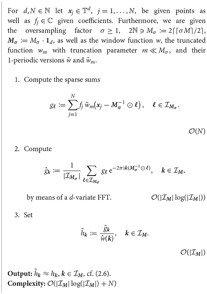
Algorithm 2.4. Adjoint NFFT.

The algorithms presented in this section (Algorithms 2.1 and 2.4) are part of the NFFT software [42]. For algorithmic details we refer to Keiner et al. [38].

3. Direct inversion using density compensation

Having introduced the fast methods for nonequispaced data, we remark that various applications such as MRI and solution of PDEs are interested in the inverse problem, i.e., instead of the evaluation of (2.5) the aim was to compute the Fourier coefficients ${\widehat{f}}_k$, $k\in {\mathcal{I}}_M$, from given nonequispaced data f(x_j), j = 1,…, N. Therefore, this section shall be dedicated to this task.

To clarify the major dissimilarity between equispaced and nonequispaced data, we start considering the equispaced case. When evaluating at the points $x_j=\frac{1}{n}j\in T^d$, $j\in {\mathcal{I}}_n$, with n := n·1_d and $\left|{\mathcal{I}}_n\right|=N$, the nonequispaced Fourier matrix $A\in {ℂ}^{N\times \left|{\mathcal{I}}_M\right|}$ in (2.7) turns into the equispaced Fourier matrix $F\in {ℂ}^{\left|{\mathcal{I}}_{M_{\sigma }}\right|\times \left|{\mathcal{I}}_M\right|}$ from (2.14) with $\left|{\mathcal{I}}_{M_{\sigma }}\right|=N$. Thereby, it results from the geometric sum formula that

$\begin{array}{ll}{F}^{*}F={({\displaystyle \sum _{j\in I_n}}{\text{e}}^{2\pi \text{i}(k-\text{ℓ})j/n})}_{k,\text{ℓ}\in I_M}=N{I}_{\left|I_M\right|},\text{\hspace{1em}if}\left|I_M\right|\le N,& (3.1)\end{array}$

as well as

$\begin{array}{ll}F{F}^{*}={\left({\displaystyle \sum _{k\in I_M}}{\text{e}}^{2\pi \text{i}k(j-h)/n}\right)}_{j,h\in I_n}=\left|I_M\right|·I_N,\text{\hspace{1em}if}\left|I_M\right|\ge N& (3.2)\end{array}$

and $\left|{\mathcal{I}}_M\right|$ is divisible by N. Thus, in the equispaced setting a one-sided inverse is given by the (scaled) adjoint matrix. However, when considering arbitrary points $x_j\in {𝕋}^d$, j = 1,…, N, this property is lost, i.e., for the nonequispaced Fourier matrix, we have

$\begin{array}{ll}{A}^{*}A\ne N{I}_{\left|I_M\right|}\text{\hspace{1em}and\hspace{1em}}A{A}^{*}\ne \left|I_M\right|·I_N.& (3.3)\end{array}$

Because of this, more effort is needed in the nonequispaced setting.

In general, we face the following two problems.

(1) Solve the linear system

$\begin{array}{ll}\begin{array}{c}A\widehat{f}=f,\end{array}& (3.4)\end{array}$

i.e., reconstruct the Fourier coefficients $\widehat{f}={({\widehat{f}}_k)}_{k\in {\mathcal{I}}_M}$ from given function values $f={(f(x_j))}_{j=1}^N$. This problem is referred to as inverse NDFT (iNDFT) and an efficient solver shall be called inverse NFFT (iNFFT).

(2) Solve the linear system

$\begin{array}{ll}\begin{array}{c}{A}^{*}f=h,\end{array}& (3.5)\end{array}$

i.e., reconstruct the coefficients $f={(f_j)}_{j=1}^N$ from given data $h={(h_k)}_{k\in {\mathcal{I}}_M}$. This problem is referred to as inverse adjoint NDFT (iNDFT*) and an efficient solver shall be called inverse adjoint NFFT (iNFFT*).

Note that in both problems the numbers $\left|{\mathcal{I}}_M\right|$ and N are independent, such that the nonequispaced Fourier matrix $A\in {ℂ}^{N\times \left|{\mathcal{I}}_M\right|}$ in (2.7) is generally rectangular.

At first, we restrict our attention to the problem (3.4). When considering iterative inversion procedures as those mentioned in the introduction, these methods require multiple iteration steps by definition. Therefore, multiple matrix-vector multiplications with the system matrix A, or rather multiple applications of the NFFT (see Algorithm 2.1), are needed to compute a solution. To reduce the computational effort, we now proceed, in contrast to this iterated procedure, with so-called direct methods. In the setting of the problem (3.4) we hereby mean methods, where for a fixed set of points x_j, j = 1,…, N, the reconstruction of $\widehat{f}$ from given f can be realized with the same number of arithmetic operations as a single application of an adjoint NFFT (see Algorithm 2.4). To achieve this, a certain precomputational step is compulsory, since the adjoint NFFT does not yield an inversion of the NFFT per se, see (3.3). Although these precomputations might be rather costly, they need to be done only once for a given set of points x_j, j = 1,…, N. In fact, the actual reconstruction step is very efficient. Therefore, direct methods are especially beneficial in case we are given fixed points for several measurement vectors f.

In this section, we focus on a direct inversion method for solving problem (3.4) that utilizes so-called sampling density compensation. To this end, we consider the integral (2.2) and introduce a corresponding quadrature formula. In contrast to the already known equispaced approximation (2.3) we now assume given arbitrary, nonequispaced points $x_j\in {𝕋}^d$, j = 1,…, N. Thereby, the Fourier coefficients (2.2) are approximated by a general quadrature rule using quadrature weights w_j ∈ ℂ, j = 1,…, N, which are needed for sampling density compensation due to the nonequispaced sampling. Thus, for a trigonometric polynomial (2.8), we have

$\begin{array}{ll}{\widehat{f}}_k=c_k(f)\approx h_k^{\text{w}}:\; ={\displaystyle \sum _{j=1}^N}{w}_{j}f(x_j){\text{e}}^{-2\pi \text{i}k{x}_j},k\in I_M.& (3.6)\end{array}$

Using the nonequispaced Fourier matrix $A\in {ℂ}^{N\times \left|{\mathcal{I}}_M\right|}$ in (2.7), the diagonal matrix of weights $W:=\text{diag}{(w_j)}_{j=1}^N\in {ℂ}^{N\times N}$ as well as the vector $h^{\text{w}}:={(h_k^{\text{w}})}_{k\in {\mathcal{I}}_M}$, the nonequispaced quadrature rule (3.6) can be written as $\widehat{f}\approx h^{\text{w}}:=A^{*}Wf$. For achieving a fast computation method, we make use of the approximation of the adjoint NFFT, cf. Section 2.2, i.e., the final approximation is given by

$\begin{array}{ll}\widehat{f}\approx {\tilde{h}}^{\text{w}}:\; =D^{*}{F}^{*}{B}^{*}Wf,& (3.7)\end{array}$

with the matrices $D\in {ℂ}^{\left|{\mathcal{I}}_M\right|\times \left|{\mathcal{I}}_M\right|}$, $F\in {ℂ}^{\left|{\mathcal{I}}_{M_{\sigma }}\right|\times \left|{\mathcal{I}}_M\right|}$, and $B\in {ℝ}^{N\times \left|{\mathcal{I}}_{M_{\sigma }}\right|}$ defined in (2.13), (2.14), and (2.15). In other words, for density compensation methods the already mentioned precomputations consists of computing the quadrature weights w_j ∈ ℂ, j = 1,…, N, while the actual reconstruction step includes only one adjoint NFFT (see Algorithm 2.4) applied to the scaled measurement vector Wf.

The aim of all density compensation techniques was then to choose appropriate weights w_j ∈ ℂ, j = 1,…, N, such that the underlying quadrature (3.6) is preferably exact. In the following, we have a look at the specific choice of the so-called density compensation factors w_j.

An intuitive approach for density compensation is based on geometry, where each sample is considered as representative of a certain surrounding area, as in numerical integration. The weights for each sample can be obtained for instance by constructing a Voronoi diagram and calculating the area of each cell, see e.g., [43]. This approach of Voronoi weights is well-known and widely used in practice. However, it does not necessarily yield a good approximation (3.7), which is why we examine some more sophisticated approaches in the remainder of this section.

To this end, this section is organized as follows. First, in Section 3.1, we introduce density compensation factors w_j, j = 1,…, N, that lead to an exact reconstruction formula (3.6) for all trigonometric polynomials (2.8) of degree M. In addition to the theoretical results, we also discuss methods for the numerical computation. Secondly, in Section 3.2, we show that it is reasonable to consider the inversion problem (3.4) and density compensation via (3.7) for bandlimited functions $f\in L_1({ℝ}^d)\cap C_0({ℝ}^d)$ as well. Subsequently, we summarize our previous findings by presenting a general error bound on density compensation factors in Section 3.3. Finally, in Section 3.4, we reconsider certain approaches from literature and illustrate their connection to each other as well as to the method introduced in Section 3.1.

Remark 3.1. Recapitulating, we have a closer look at some possible interpretation perspectives on the reconstruction (3.7).

(i) If we define g := Wf, i.e., each entry of f is scaled with respect to the points x_j, j = 1,…, N, the approximation (3.7) can be written as $\widehat{f}\approx D^{*}{F}^{*}{B}^{*}g$. As mentioned before, this coincides with an ordinary adjoint NFFT applied to a modified coefficient vector g.

(ii) By defining the matrix $\tilde{B}:=W^{*}B$, i.e., scaling the rows of B with respect to the points x_j, j = 1, …, N, the approximation (3.7) can be written as $\widehat{f}\approx D^{*}{F}^{*}{\tilde{B}}^{*}f$. In this sense, density compensation can also be seen as a modification of the adjoint NFFT and its application to the original coefficient vector.

Note that (i) is the common viewpoint. However, we keep (ii) in mind, since this allows treating density compensation methods as an optimization of the sparse matrix $B\in {ℝ}^{N\times \left|{\mathcal{I}}_{M_{\sigma }}\right|}$ in (2.15), as it shall be done in Section 4. We remark that density compensation methods allow only N degrees of freedom.□

3.1. Exact quadrature weights for trigonometric polynomials

Similar to Gräf et al. [44], we aimed to introduce density compensation factors w_j, j = 1,…, N, that lead to an exact reconstruction formula (3.6) for all trigonometric polynomials (2.8) of degree M. To this end, we first examine certain properties that arise from (3.6) being exact.

Theorem 3.2. Let a polynomial degree M ∈ (2ℕ)^d, nonequispaced points $x_j\in T^d$, j = 1, …, N, and quadrature weights w_j ∈ ℂ be given. Then an exact reconstruction formula (3.6) for trigonometric polynomials (2.8) with maximum degree M satisfying

$\begin{array}{ll}{\widehat{f}}_k=c_k(f)=h_k^{\text{w}},k\in I_M,& (3.8)\end{array}$

implies the following equivalent statements.

(i) The quadrature rule

$\begin{array}{ll}{\displaystyle {\int }_{{𝕋}^d}}f(x)\text{d}x={\displaystyle \sum _{j=1}^N}{w}_{j}f(x_j)& (3.9)\end{array}$

is exact for all trigonometric polynomials (2.8) with maximum degree M.

(ii) The linear system of equations

$\begin{array}{l}{\left[A^{T}w\right]}_k={\displaystyle \sum _{j=1}^N}{w}_j{\text{e}}^{2\pi \text{i}k{x}_j}={\delta }_{0,k}=\left\{\begin{array}{cc}1& :k=0\hfill \\ 0& :\text{otherwise}\end{array}\right\},\\ \hfill k\in I_M,& (3.10)\end{array}$

is fulfilled with the matrix $A\in {ℂ}^{N\times \left|{\mathcal{I}}_M\right|}$ in (2.7) and $w:={(w_j)}_{j=1}^N$.

Proof: (3.8) ⇒ (i): By inserting the definition (2.8) of a trigonometric polynomial of degree M into the integral considered in (3.9), we have

$\begin{array}{ll}{\displaystyle {\int }_{{𝕋}^d}}f(x)\text{d}x={\displaystyle \sum _{k\in I_M}}{\widehat{f}}_k·{\displaystyle {\int }_{{𝕋}^d}}{\text{e}}^{2\pi \text{i}kx}\text{d}x={\displaystyle \sum _{k\in I_M}}{\widehat{f}}_k·{\delta }_{0,k}={\widehat{f}}_0,& (3.11)\end{array}$

with the Kronecker delta δ_0,k. Now using the property (3.8) as well as definition (3.6) of $h_k^{\text{w}}$ we proceed with

$\begin{array}{ll}{\widehat{f}}_0=h_0^{\text{w}}={\displaystyle \sum _{j=1}^N}{w}_{j}f(x_j){\displaystyle \sum _{k\in I_M}}{\text{e}}^0={\displaystyle \sum _{j=1}^N}{w}_{j}f(x_j),& (3.12)\end{array}$

such that (3.11) combined with (3.12) yields the assertion (3.9).

(i) ⇒ (ii): Inserting the definition (2.8) of a trigonometric polynomial of degree M into the right-hand side of (3.9) implies

$\begin{array}{ll}{\displaystyle \sum _{j=1}^N}{w}_{j}f(x_j)={\displaystyle \sum _{j=1}^N}{w}_j{\displaystyle \sum _{k\in I_M}}{\widehat{f}}_k{\text{e}}^{2\pi \text{i}k{x}_j}={\displaystyle \sum _{k\in I_M}}{\widehat{f}}_k{\displaystyle \sum _{j=1}^N}{w}_j{\text{e}}^{2\pi \text{i}k{x}_j}.& (3.13)\end{array}$

This together with the property (i) and (3.11) leads to

$\begin{array}{l}{\widehat{f}}_0={\displaystyle \sum _{k\in I_M}}{\widehat{f}}_k{\displaystyle \sum _{j=1}^N}{w}_j{\text{e}}^{2\pi \text{i}k{x}_j}\end{array}$

and thus to assertion (3.10).

(ii) ⇒ (i): Combining (3.11), (3.10), and (3.13) yields the assertion via

$\begin{array}{l}{\displaystyle {\int }_{{𝕋}^d}}f(x)\text{d}x={\displaystyle \sum _{k\in I_M}}{\widehat{f}}_k·{\delta }_{0,k}={\displaystyle \sum _{k\in I_M}}{\widehat{f}}_k{\displaystyle \sum _{j=1}^N}{w}_j{\text{e}}^{2\pi \text{i}k{x}_j}={\displaystyle \sum _{j=1}^N}{w}_{j}f(x_j).\end{array}$

□

Remark 3.3. Comparable results can also be found in literature. A fundamental theorem in numerical integration, see [45], states that for any integral ${\int }_{{𝕋}^d}f(x)dx$ there exists an exact quadrature rule (3.9), i.e., optimal points $x_j\in {𝕋}^d$ and weights w_j ∈ ℂ, j = 1,…, N, such that (3.9) is fulfilled. In Gröchenig [46, Lemma 2.6], it was shown that for given points $x_j\in {𝕋}^d$, j = 1,…, N, certain quadrature weights w_j can be stated by means of frame theoretical considerations that lead to an exact quadrature rule (3.9) by definition. Moreover, it was shown (cf. [46, Lemma 3.6]) that these weights are the ones with minimal (weighted) ℓ₂-norm, which are already known under the name “least squares quadrature,” see [47]. According to Huybrechs [47, Sec. 2.1], these quadrature weights w_j, j = 1,…, N, can be found by solving a linear system of equations Φw = v, where Φ_{k, j} = ϕ_k(x_j) and $v_k={\int }_{{𝕋}^d}{\varphi }_k(x)dx$ for a given set of basis functions ${\left\{{\varphi }_k\right\}}_{k\in {\mathcal{I}}_M}$. In our setting, we have ${\varphi }_k(x)={\text{e}}^{2\pi \text{i}kx}$ and, therefore,

$\begin{array}{l}\Phi ={\left({\text{e}}^{2\pi \text{i}k{x}_j}\right)}_{k,j}=A^T\text{\hspace{1em}and\hspace{1em}}{v}_k={\displaystyle {\int }_{{𝕋}^d}}1·{\text{e}}^{2\pi \text{i}kx}\text{d}x={\delta }_{0,k},\end{array}$

i.e., the same linear system of equations as in (3.10). We remark that both Gröchenig [46] and Huybrechs [47] state the results in the case d = 1, a generalization to d > 1, however, is straight-forward.□

By means of Theorem 3.2 we can now give a condition that guarantees (3.6) being exact for all trigonometric polynomials (2.8) with maximum degree M.

Corollary 3.4. The two statements (i) and (ii) in Theorem 3.2 are not equivalent to property (3.8), since (3.10) does not imply an exact reconstruction in (3.6).

However, an augmented variant of (3.10), namely,

$\begin{array}{ll}{\displaystyle \sum _{j=1}^N}{w}_j{\text{e}}^{2\pi \text{i}k{x}_j}={\delta }_{0,k},k\in I_{2M},& (3.14)\end{array}$

yields an exact reconstruction ${\widehat{f}}_k=h_k^{\text{w}}$ in (3.6) for trigonometric polynomials (2.8) with maximum degree M. In addition, (3.14) implies the matrix equation $A^{*}WA=I_{\left|{\mathcal{I}}_M\right|}$ with $A\in {ℂ}^{N\times \left|{\mathcal{I}}_M\right|}$ in (2.7) and the identity matrix $I_{\left|{\mathcal{I}}_M\right|}$ of size $\left|{\mathcal{I}}_M\right|$.

Proof: Utilizing definitions (3.6) and (2.8), we have

$\begin{array}{l}{h}_k^{\text{w}}={\displaystyle \sum _{j=1}^N}{w}_j\left({\displaystyle \sum _{\text{ℓ}\in I_M}}{\widehat{f}}_{\text{ℓ}}{\text{e}}^{2\pi \text{i}\text{ℓ}{x}_j}\right){\text{e}}^{-2\pi \text{i}k{x}_j}\\ ={\displaystyle \sum _{\text{ℓ}\in I_M}}{\widehat{f}}_{\text{ℓ}}{\displaystyle \sum _{j=1}^N}{w}_j{\text{e}}^{2\pi \text{i}(\text{ℓ}-k)x_j}\\ ={\displaystyle \sum _{\begin{array}{c}\text{ℓ}\in I_M\\ (\text{ℓ}-k)\in I_M\end{array}}}{\widehat{f}}_{\text{ℓ}}{\displaystyle \sum _{j=1}^N}{w}_j{\text{e}}^{2\pi \text{i}(\text{ℓ}-k)x_j}\\ +{\displaystyle \sum _{\begin{array}{c}\text{ℓ}\in I_M\\ (\text{ℓ}-k)\notin I_M\end{array}}}{\widehat{f}}_{\text{ℓ}}{\displaystyle \sum _{j=1}^N}{w}_j{\text{e}}^{2\pi \text{i}(\text{ℓ}-k)x_j},k\in I_M.\end{array}$

Since (3.10) only holds for $k,\ell \in {\mathcal{I}}_M$ with $(\ell -k)\in {\mathcal{I}}_M$, this implies

$\begin{array}{l}{h}_k^{\text{w}}={\widehat{f}}_k+{\displaystyle \sum _{\begin{array}{c}\text{ℓ}\in I_M\\ (\text{ℓ}-k)\notin I_M\end{array}}}{\widehat{f}}_{\text{ℓ}}{\displaystyle \sum _{j=1}^N}{w}_j{\text{e}}^{2\pi \text{i}(\text{ℓ}-k)x_j},k\in I_M,\end{array}$

where for all $k\in {\mathcal{I}}_M\backslash \left\{0\right\}$ there exists an $\ell \in {\mathcal{I}}_M$ with $(\ell -k)\in {\mathcal{I}}_{2M}\backslash {\mathcal{I}}_M$.

As $(\ell -k)\in {\mathcal{I}}_{2M}$ for $k,\ell \in {\mathcal{I}}_M$, the augmented variant (3.14) yields

$\begin{array}{l}{h}_k^{\text{w}}={\displaystyle \sum _{\text{ℓ}\in I_M}}{\widehat{f}}_{\text{ℓ}}{\displaystyle \sum _{j=1}^N}{w}_j{\text{e}}^{2\pi \text{i}(\text{ℓ}-k)x_j}={\displaystyle \sum _{\text{ℓ}\in I_M}}{\widehat{f}}_k·{\delta }_{0,k}={\widehat{f}}_k,k\in I_M.\end{array}$

Moreover, since δ_{(ℓ−k), 0} = δ_k,ℓ, the condition (3.14) implies

$\begin{array}{l}{\delta }_{k,\text{ℓ}}={\displaystyle \sum _{j=1}^N}{w}_j{\text{e}}^{2\pi \text{i}(\text{ℓ}-k)x_j}={\displaystyle \sum _{j=1}^N}{\text{e}}^{-2\pi \text{i}k{x}_j}\left(w_j{\text{e}}^{2\pi \text{i}\text{ℓ}{x}_j}\right),k,\text{ℓ}\in I_M.\end{array}$

In matrix-vector notation, this can be written as $A^{*}WA=I_{\left|{\mathcal{I}}_M\right|}$ with $A\in {ℂ}^{N\times \left|{\mathcal{I}}_M\right|}$ in (2.7) and the identity matrix $I_{\left|{\mathcal{I}}_M\right|}$ of size $\left|{\mathcal{I}}_M\right|$. We remark that this matrix equation immediately shows that we have an exact reconstruction of the form (3.8), since if $A^{*}WA=I_{\left|{\mathcal{I}}_M\right|}$ is fulfilled, (3.4) implies that $\widehat{f}=A^{*}WA\widehat{f}=A^{*}Wf$.□

Remark 3.5. Let $f\in L_2({𝕋}^d)$ be an arbitrary 1-periodic function (2.1). Then (3.14) yields

$\begin{array}{l}{h}_k^{\text{w}}={\displaystyle \sum _{\text{ℓ}\in {\mathbb{Z}}^d}}{c}_{\text{ℓ}}(f){\displaystyle \sum _{j=1}^N}{w}_j{\text{e}}^{2\pi \text{i}(\text{ℓ}-k)x_j}={\displaystyle \sum _{\begin{array}{c}\text{ℓ}\in {\mathbb{Z}}^d\\ (\text{ℓ}-k)\in I_{2M}\end{array}}}{c}_{\text{ℓ}}(f){\displaystyle \sum _{j=1}^N}{w}_j{\text{e}}^{2\pi \text{i}(\text{ℓ}-k)x_j}\\ +{\displaystyle \sum _{\begin{array}{c}\text{ℓ}\in {\mathbb{Z}}^d\\ (\text{ℓ}-k)\notin I_{2M}\end{array}}}{c}_{\text{ℓ}}(f){\displaystyle \sum _{j=1}^N}{w}_j{\text{e}}^{2\pi \text{i}(\text{ℓ}-k)x_j}\\ =c_k(f)+{\displaystyle \sum _{\begin{array}{c}\text{ℓ}\in {\mathbb{Z}}^d\\ (\text{ℓ}-k)\notin I_{2M}\end{array}}}{c}_{\text{ℓ}}(f){\displaystyle \sum _{j=1}^N}{w}_j{\text{e}}^{2\pi \text{i}(\text{ℓ}-k)x_j},k\in I_M,\end{array}$

i.e., for a function $f\in L_2({𝕋}^d)$ we only have a good approximation in case the coefficients c_ℓ(f) are small for $\ell \notin {\mathcal{I}}_M$, whereas this reconstruction can only be exact for f being a trigonometric polynomial (2.8).□

3.1.1. Practical computation in the underdetermined setting $\left|{\mathcal{I}}_{2M}\right|\le N$

So far, we have seen in Corollary 3.4 that an exact solution $w={(w_j)}_{j=1}^N$ to the linear system (3.14) leads to an exact reconstruction formula (3.6) for all trigonometric polynomials (2.8) with maximum degree M. Therefore, we aimed to use this condition (3.14) to numerically find optimal density compensation factors w_j ∈ ℂ, j = 1,…, N.

Having a closer look at the condition (3.14) we recognize that it can be written as the linear system of equations ${\mathit{A}}_{\left|{\mathcal{I}}_{2M}\right|}^T\mathit{w}={\mathit{e}}_{\mathbf{0}}$ with the matrix $A_{\left|{\mathcal{I}}_{2M}\right|}\in {ℂ}^{N\times \left|{\mathcal{I}}_{2M}\right|}$, cf. (2.7), and right side $e_0:={({\delta }_{0,k})}_{k\in {\mathcal{I}}_{2M}}$. We remark that in contrast to $A\in {ℂ}^{N\times \left|{\mathcal{I}}_M\right|}$ we now deal with the enlarged matrix $A_{\left|{\mathcal{I}}_{2M}\right|}\in {ℂ}^{N\times \left|{\mathcal{I}}_{2M}\right|}$, such that single matrix operations are more costly. Nevertheless, Corollary 3.4 yields a direct inversion method for (3.4), where the system ${\mathit{A}}_{\left|{\mathcal{I}}_{2M}\right|}^T\mathit{w}={\mathit{e}}_{\mathbf{0}}$ needs to be solved only once for fixed points $x_j\in {𝕋}^d$, j = 1,…, N. Its solution w can then be used to efficiently approximate $\widehat{f}$ for multiple measurement vectors f, whereas iterative methods for (3.4) need to solve $A\widehat{f}=f$ each time.

As already mentioned in [47, Sec. 3.1] an exact solution to (3.14) can only be found if $\left|{\mathcal{I}}_{2M}\right|\le N$, i.e., in case ${\mathit{A}}_{\left|{\mathcal{I}}_{2M}\right|}^T\mathit{w}={\mathit{e}}_{\mathbf{0}}$ is an underdetermined system of equations. By [47, Lem. 3.1] this system has at least one solution, which is why we may choose the one with a minimal ℓ₂-norm. If $\text{rank}({\mathit{A}}_{\left|{\mathcal{I}}_{2M}\right|})=\left|{\mathcal{I}}_{2M}\right|$, then the system ${\mathit{A}}_{\left|{\mathcal{I}}_{2M}\right|}^T\mathit{w}={\mathit{e}}_{\mathbf{0}}$ is consistent and the unique solution is given by the normal equations of the second kind

$\begin{array}{ll}{A}_{\left|I_{2M}\right|}^T\overline{A_{\left|I_{2M}\right|}}v=e_0,\overline{A_{\left|I_{2M}\right|}}v=w.& (3.15)\end{array}$

More precisely, we may compute the vector v using an iterative procedure such as the CG algorithm, such that only matrix multiplications with ${\mathit{A}}_{\left|{\mathcal{I}}_{\mathit{2}\mathit{M}}\right|}^T$ and $\overline{{\mathit{A}}_{\left|{\mathcal{I}}_{\mathit{2}\mathit{M}}\right|}}$ are needed. Since fast multiplication with ${\mathit{A}}_{\left|{\mathcal{I}}_{\mathit{2}\mathit{M}}\right|}^T$ and $\overline{{\mathit{A}}_{\left|{\mathcal{I}}_{\mathit{2}\mathit{M}}\right|}}$ can easily be realized by means of an adjoint NFFT (see Algorithm 2.4) and an NFFT (see Algorithm 2.1), respectively, computing the solution w to (3.15) is of complexity $\mathcal{O}(|I_{\mathit{2}\mathit{M}}|\log (\left|I_{\mathit{2}\mathit{M}}\right|)+N)$, where

$\begin{array}{l}\left|I_{2M}\right|={(2M)}^d=2^d{M}^d=2^d\left|I_M\right|.\end{array}$

Thus, to receive exact quadrature weights w_j ∈ ℂ, j = 1,…, N, via (3.15) we need to satisfy the full rank condition $\text{rank}({\mathit{A}}_{\left|{\mathcal{I}}_{\mathit{2}\mathit{M}}\right|})=\left|{\mathcal{I}}_{2M}\right|$. In case of a low-rank matrix $A_{\left|{\mathcal{I}}_{2M}\right|}\in {ℂ}^{N\times \left|{\mathcal{I}}_{2M}\right|}$ for $\left|{ℐ}_{\mathit{2}\mathit{M}}\right|\le N$, we may still use (3.15) to obtain a least squares approximation to (3.14).

3.1.2. Practical computation in the overdetermined setting $\left|{ℐ}_{\mathit{2}\mathit{M}}\right|>N$

In the setting $\left|{ℐ}_{\mathit{2}\mathit{M}}\right|>N$, we cannot expect to find an exact solution w to (3.14), since we have to deal with an overdetermined system possessing more conditions than variables. However, we still aimed to numerically find optimal density compensation factors w_j∈ℂ, j = 1,…, N, by considering a least squares approximation to (3.14) that minimizes $\Vert {\mathit{A}}_{\left|{ℐ}_{\mathit{2}\mathit{M}}\right|}^{\mathcal{T}}\mathit{w}- {\mathit{e}}_{\mathit{0}}{\Vert }_2$. In [60, Thm. 1.1.2] it was shown that every least squares solution satisfies the normal equations of the first kind

$\begin{array}{ll}\overline{A_{\left|I_{2M}\right|}}{A}_{\left|I_{2\mathrm{M}}\right|}^{T}w=\overline{A_{\left|I_{2M}\right|}}{e}_0.& (3.16)\end{array}$

By means of definitions of ${\mathit{A}}_{\left|{\mathcal{I}}_{\mathit{2}\mathit{M}}\right|}\in {\text{ℂ}}^{N\times \left|{\mathcal{I}}_{\mathit{2}\mathit{M}}\right|}$, cf. (2.7), and $e_0={({\delta }_{0,k})}_{k\in {\mathcal{I}}_{2M}}$ we simplify the right-hand side via

$\begin{array}{l}\overline{A_{\left|I_{2M}\right|}}{e}_0=({\displaystyle \sum _{k\in I_{2M}}}{\delta }_{0,k}{\text{e}}^{-2\pi \text{i}k{x}_j}{)}_{j=1}^N=1_N.\end{array}$

Since fast multiplication with ${\mathit{A}}_{\left|I_{\mathit{2}\mathit{M}}\right|}^T$ and $\overline{{\mathit{A}}_{\left|{\mathcal{I}}_{\mathit{2}\mathit{M}}\right|}}$ can easily be realized by means of an adjoint NFFT (see Algorithm 2.4) and an NFFT (see Algorithm 2.1), respectively, the solution w to (3.16) can be computed iteratively by means of the CG algorithm in $\mathcal{O}(|{\mathcal{I}}_{2M}|\log (\left|{\mathcal{I}}_{\mathit{2}\mathit{M}}\right|)+N)$ arithmetic operations. Note that the solution to (3.16) is only unique if the full rank condition $\text{rank}(A_{\left|{\mathcal{I}}_{\mathit{2}\mathit{M}}\right|})=N$ is satisfied, cf. [60, p. 7]. We remark that the computed weight matrix W = diag(w) can further be used in an iterative procedure as in Plonka et al. [[15, Alg. 7.27] to improve the approximation of $\widehat{f}$.

The previous considerations lead to the following algorithms.

ALGORITHM 3.6

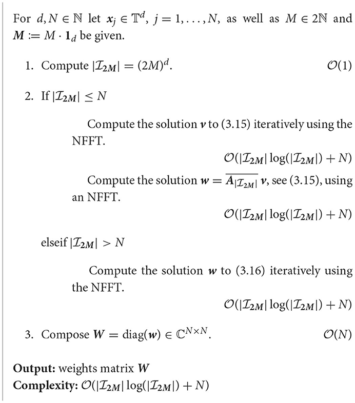
Algorithm 3.6. Computation of the optimal density compensation factors.

ALGORITHM 3.7

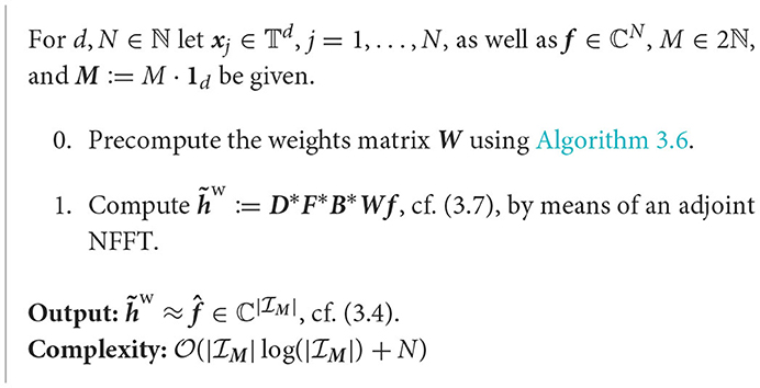
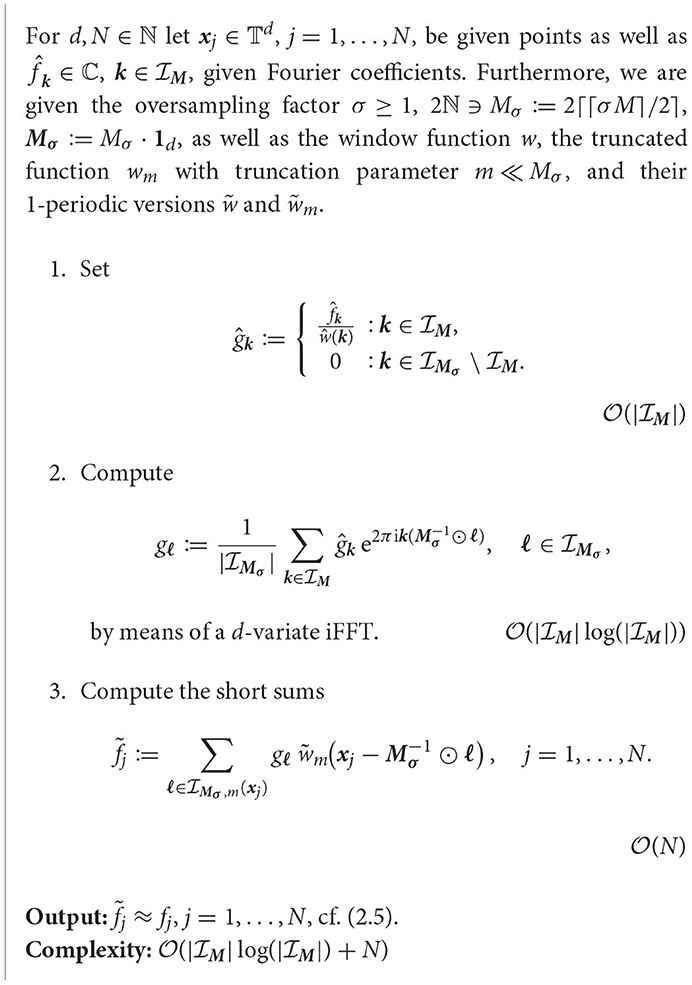
Algorithm 3.7. iNFFT – density compensation approach.

3.2. Bandlimited functions

In some numerical examples, such as in MRI, we are concerned with bandlimited functions $f\in L_1({ℝ}^d)\cap C_0({ℝ}^d)$ instead of trigonometric polynomials $f\in L_2({𝕋}^d)$ in (2.8), cf. [1]. In the following we show that it is reasonable to consider the inversion problem (3.4) as well as the density compensation via (3.7) for bandlimited functions as well.

To this end, let $f\in L_1({ℝ}^d)\cap C_0({ℝ}^d)$ be a bandlimited function with bandwidth M, i.e., its (continuous) Fourier transform

$\begin{array}{ll}\widehat{f}(v):\; ={\displaystyle \underset{{ℝ}^d}{\int }}f(x){\text{e}}^{-2\pi \text{i}vx}\text{d}x,v\in {ℝ}^d,& (3.17)\end{array}$

is supported on ${\left[-\frac{M}{2},\frac{M}{2}\right)}^d$. Utilizing this fact, we have $\widehat{f}\in L_1({ℝ}^d)$ and thus by the Fourier inversion theorem [15, Thm. 2.10] the inverse Fourier transform of f can be written as

$\begin{array}{ll}f(x)={\displaystyle \underset{{ℝ}^d}{\int }}\widehat{f}(v){\text{e}}^{2\pi \text{i}vx}\text{d}v={\displaystyle \underset{[-\frac{M}{2},\frac{M}{2}{)}^d}{\int }}\widehat{f}(v){\text{e}}^{2\pi \text{i}vx}\text{d}v,x\in {ℝ}^d.& (3.18)\end{array}$

Analogous to (2.3), the approximation using equispaced quadrature points $k\in {\mathcal{I}}_M$ yields

$\begin{array}{l}f(x)\approx \frac{{\left(\frac{M}{2}-(-\frac{M}{2})\right)}^d}{\left|I_M\right|}{\displaystyle \sum _{k\in I_M}}\widehat{f}(k){\text{e}}^{2\pi \text{i}kx}={\displaystyle \sum _{k\in I_M}}\widehat{f}(k){\text{e}}^{2\pi \text{i}kx},\\ \hfill x\in {ℝ}^d,& (3.19)\end{array}$

such that evaluation at the given nonequispaced points ${\mathit{x}}_j\in {\left[-\frac{1}{2},\frac{1}{2}\right)}^d$, j = 1,…, N, leads to

$\begin{array}{l}f(x_j)\approx {\displaystyle \sum _{k\in I_M}}\widehat{f}(k){\text{e}}^{2\pi \text{i}k{x}_j}.\end{array}$

By means of the definition (2.7) of the matrix $A\in {ℂ}^{N\times \left|{\mathcal{I}}_M\right|}$ this can be written as $f\approx A\widehat{f}$, where we used the notation $\widehat{f}:={(\widehat{f}(k))}_{k\in {\mathcal{I}}_M}$ in this setting. Thus, also for bandlimited functions f its evaluations at points x_j can be approximated in the form (2.5), such that it is reasonable to consider the inversion problem (3.4) for bandlimited functions as well.

Considering (3.17) we are given an exact formula for the evaluation of the Fourier transform $\widehat{f}$. However, in practical applications, such as MRI, this is only a hypothetical case, since f cannot be sampled on whole ℝ^d, cf. [1]. Due to a limited coverage of space by the acquisition, the function f is typically only known on a bounded domain, w.l.o.g. for ${\mathit{x}}_j\in {\left[-\frac{1}{2},\frac{1}{2}\right)}^d$. Thus, we have to deal with the approximation

$\begin{array}{ll}\widehat{f}(v)\approx {\displaystyle \underset{[-\frac{1}{2},\frac{1}{2}{)}^d}{\int }}f(x){\text{e}}^{-2\pi \text{i}vx}\text{d}x,v\in [-\frac{M}{2},\frac{M}{2}{)}^d.& (3.20)\end{array}$

Using the nonequispaced quadrature rule in (3.6), we find that evaluation at uniform grid points $k\in {\mathcal{I}}_M$ can be approximated via

$\begin{array}{l}\widehat{f}(k)\approx \tilde{h}(k):\; ={\displaystyle \sum _{j=1}^N}{w}_{j}f(x_j){\text{e}}^{-2\pi \text{i}k{x}_j},k\in I_M.\end{array}$

This is to say, equispaced samples of the Fourier transform of a bandlimited function may be approximated in the same form ${(\widehat{f}(k))}_{k\in {\mathcal{I}}_M}=\widehat{f}\approx h^{\text{w}}:=A^{*}Wf$ as in (3.6), where we used the notation $h^{\text{w}}:={(\tilde{h}(k))}_{k\in {\mathcal{I}}_M}$ in this setting. Moreover, we extend this approximation onto the whole interval ${\left[-\frac{M}{2},\frac{M}{2}\right)}^d$, i.e., we consider

$\begin{array}{ll}\widehat{f}(v)\approx \tilde{h}(v):\; ={\displaystyle \sum _{j=1}^N}{w}_{j}f(x_j){\text{e}}^{-2\pi \text{i}v{x}_j},v\in [-\frac{M}{2},\frac{M}{2}{)}^d.& (3.21)\end{array}$

So all in all, we have seen that it is reasonable to study the inversion problem (3.4) and the associated density compensation via (3.7) for bandlimited functions as well. Analogous to Section 3.1, we now aimed to find a numerical method for computing suitable weights w_j ∈ ℂ, j = 1,…, N, such that the reconstruction formula (3.21) is preferably exact. To this end, we have a closer look at (3.21) being exact and start with analogous considerations as in Theorem 3.2.

Theorem 3.8. Let a bandwidth M ∈ ℕ^d, nonequispaced points ${\mathit{x}}_j\in {\left[-\frac{1}{2},\frac{1}{2}\right)}^d$ as well as quadrature weights w_j ∈ ℂ, j = 1,…, N, be given. Then an exact reconstruction formula (3.21) for bandlimited functions $f\in L_1({ℝ}^d)\cap C_0({ℝ}^d)$ with bandwidth M, i.e.,

$\begin{array}{ll}\widehat{f}(v)=\tilde{h}(v)={\displaystyle \sum _{j=1}^N}{w}_{j}f(x_j){\text{e}}^{-2\pi \text{i}v{x}_j},v\in [-\frac{M}{2},\frac{M}{2}{)}^d,& (3.22)\end{array}$

implies that the quadrature rule

$\begin{array}{l}{\displaystyle {\int }_{{ℝ}^d}}f(x)\text{d}x={\displaystyle \sum _{j=1}^N}{w}_{j}f(x_j)\end{array}$

is exact for all bandlimited functions $f\in L_1({ℝ}^d)\cap C_0({ℝ}^d)$ with bandwidth M.

Proof: By (3.17) the assumption (3.22) can be written as

$\begin{array}{l}{\displaystyle \underset{{ℝ}^d}{\int }}f(x){\text{e}}^{-2\pi \text{i}vx}\text{d}x=\widehat{f}(v)={\displaystyle \sum _{j=1}^N}{w}_{j}f(x_j){\text{e}}^{-2\pi \text{i}v{x}_j},\\ \hfill v\in [-\frac{M}{2},\frac{M}{2}{)}^d.& (3.23)\end{array}$

Especially, for v = 0 evaluation of (3.23) yields the assertion

$\begin{array}{l}{\displaystyle \underset{{ℝ}^d}{\int }}f(x)\text{d}x=\widehat{f}(0)={\displaystyle \sum _{j=1}^N}{w}_{j}f(x_j).\end{array}$

□

However, in contrast to Theorem 3.2, this Theorem 3.8 does not yield an explicit condition for computing suitable weights w_j∈ℂ, j = 1,…, N. To derive a numerical procedure anyway, we generalize the notion of an exact reconstruction $\tilde{h}$ of f and have a look at the theory of tempered distributions. To this end, let $\mathcal{S}$(ℝ^d) be the Schwartz space of rapidly decaying functions, cf. [15, Sec. 4.2.1]. The tempered Dirac distribution δ shall be defined by $\langle \delta ,\phi \rangle :={\int }_{{ℝ}^d}\phi (v)\delta (v)dv=\phi (0)$ for all φ ∈ $\mathcal{S}$(ℝ^d), cf. [15, Ex. 4.36]. For a slowly increasing function f:ℝ^d → ℂ satisfying $\left|f(x)\right|\le c{(1+\left|\right|x|{|}_2)}^n$ almost everywhere with c > 0 and n ∈ ℕ₀, the induced distribution T_f shall be defined by $\langle T_f,\phi \rangle :=\underset{{ℝ}^d}{\int }\phi (x)f(x)dx$ for all φ ∈ $\mathcal{S}$(ℝ^d). For a detailed introduction to the topic we refer to [15, Sec. 4.2.1 and Sec. 4.3].

Then the following property can be shown.

Theorem 3.9. Let nonequispaced points ${\mathit{x}}_j\in {\left[-\frac{1}{2},\frac{1}{2}\right)}^d$, j = 1, …, N, and quadrature weights w_j ∈ ℂ be given. Furthermore, let T_f be the distribution induced by some bandlimited function $f\in L_1({ℝ}^d)\cap C_0({ℝ}^d)$ with bandwidth M. Then

$\begin{array}{ll}\langle \delta ,\phi \rangle =\langle T_{\xi },\phi \rangle ,\phi \in S({ℝ}^d),& (3.24)\end{array}$

with

$\begin{array}{ll}\xi (v):\; ={\displaystyle \sum _{j=1}^N}{w}_j{\text{e}}^{2\pi \text{i}v{x}_j},v\in {ℝ}^d,& (3.25)\end{array}$

implies

$\begin{array}{ll}\langle {\widehat{T}}_f,\phi \rangle =\langle T_{\tilde{h}},\phi \rangle ,\phi \in S({ℝ}^d),& (3.26)\end{array}$

with the function $\tilde{h}$ defined in (3.21).

Proof: Using the definition of the function $\tilde{h}$ in (3.21) as well as the fact that the inversion formula (3.18) holds for all x ∈ ℝ^d, we have

$\begin{array}{l}\langle T_{\tilde{h}},\phi \rangle ={\displaystyle {\int }_{{ℝ}^d}}\phi (v){\displaystyle \sum _{j=1}^N}{w}_{j}f(x_j){\text{e}}^{-2\pi \text{i}v{x}_j}\text{d}v\\ ={\displaystyle {\int }_{{ℝ}^d}}\phi (v){\displaystyle \sum _{j=1}^N}{w}_j\left({\displaystyle {\int }_{{ℝ}^d}}\widehat{f}(u){\text{e}}^{2\pi \text{i}u{x}_j}\text{d}u\right){\text{e}}^{-2\pi \text{i}v{x}_j}\text{d}v\\ =-{\displaystyle {\int }_{{ℝ}^d}}\widehat{f}(u){\displaystyle {\int }_{{ℝ}^d}}\phi (u-v){\displaystyle \sum _{j=1}^N}{w}_j{\text{e}}^{2\pi \text{i}v{x}_j}\text{d}v\text{d}u.\end{array}$

Hence, by (3.24), this implies

$\begin{array}{l}\langle T_{\tilde{h}},\phi \rangle =-{\displaystyle {\int }_{{ℝ}^d}}\widehat{f}(u){\displaystyle {\int }_{{ℝ}^d}}\phi (u-v)\delta (v)\text{d}v\text{d}u\\ ={\displaystyle {\int }_{{ℝ}^d}}\widehat{f}(u){\displaystyle {\int }_{{ℝ}^d}}\phi (v)\delta (u-v)\text{d}v\text{d}u={\displaystyle {\int }_{{ℝ}^d}}\widehat{f}(u)\phi (u)\text{d}u.\end{array}$

□

Considering the property (3.26), we remark that this indeed states an exact reconstruction $\widehat{f}=\tilde{h}$ in the sense of tempered distributions, as distinct from (3.22). Since it is known by Corollary 3.4 that the condition (3.14) yields an exact reconstruction for trigonometric polynomials, we aimed to use this result to compute suitable weights w_j ∈ ℂ, j = 1,…, N, for bandlimited functions as well. To this end, suppose we have (3.14), i.e.,

$\begin{array}{l}{\displaystyle \sum _{j=1}^N}{w}_j{\text{e}}^{2\pi \text{i}k{x}_j}={\delta }_{0,k},k\in I_{2M}.\end{array}$

Then this yields

$\begin{array}{ll}\phi (0)={\displaystyle \sum _{k\in I_{2M}}}\phi (k){\displaystyle \sum _{j=1}^N}{w}_j{\text{e}}^{2\pi \text{i}k{x}_j},\phi \in S({ℝ}^d).& (3.27)\end{array}$

Having a look at Theorem 3.9, an exact reconstruction (3.26) is implied by (3.24), i.e.,

$\begin{array}{l}\phi (0)=\langle \delta ,\phi \rangle =\langle T_{\xi },\phi \rangle ={\displaystyle {\int }_{{ℝ}^d}}\phi (v){\displaystyle \sum _{j=1}^N}{w}_j{\text{e}}^{2\pi \text{i}v{x}_j}\text{d}v,\phi \in S({ℝ}^d).\end{array}$

Thus, the property (3.27) that is fulfilled by (3.14) could be interpreted as an equispaced quadrature of (3.24) at integer frequencies $k\in {\mathcal{I}}_{2M}$.

Remark 3.10. We remark that for deriving the quadrature rule (3.27) from (3.24), we implicitly truncate the integral bounds in (3.24) as

$\begin{array}{l}\langle T_{\xi },\phi \rangle ={\displaystyle {\int }_{{ℝ}^d}}\phi (v){\displaystyle \sum _{j=1}^N}{w}_j{\text{e}}^{2\pi \text{i}v{x}_j}\text{d}v\\ \approx {\displaystyle \underset{[-M,M{)}^d}{\int }}\phi (v){\displaystyle \sum _{j=1}^N}{w}_j{\text{e}}^{2\pi \text{i}v{x}_j}\text{d}v\\ ={\displaystyle {\int }_{{ℝ}^d}}\phi (v){\displaystyle \sum _{j=1}^N}{w}_j{\text{e}}^{2\pi \text{i}v{x}_j}{\chi }_{[-M,M{)}^d}(v)\text{d}v,\end{array}$

i.e., instead of (3.25) we rather deal with a distribution induced by

$\begin{array}{ll}\tilde{\xi }(v):\; =\xi (v){\chi }_{[-M,M{)}^d}(v),v\in {ℝ}^d.& (3.28)\end{array}$

However, an analogous implication as in Theorem 3.9 cannot be shown when using the function (3.28) instead of (3.25).□

As seen in Remark 3.10, our numerical method for computing suitable weights w_j ∈ ℂ, j = 1,…, N, can also be derived by means of a quadrature formula applied to the property $\langle \delta ,\widehat{\phi }\rangle =\langle T_{\tilde{\xi }},\widehat{\phi }\rangle$ with $\tilde{\xi }$ defined in (3.28). Having a closer look at this property, the following equivalent characterization can be shown.

Theorem 3.11. Let a bandwidth M ∈ ℕ^d, nonequispaced points ${\mathit{x}}_j\in {\left[-\frac{1}{2},\frac{1}{2}\right)}^d$, and quadrature weights w_j ∈ ℂ, j = 1, …, N, be given. Then the following two statements are equivalent.

(i) For all φ ∈ $\mathcal{S}$(ℝ^d) we have $\langle \delta ,\widehat{\phi }\rangle =\langle T_{\tilde{\xi }},\widehat{\phi }\rangle$ with $\tilde{\xi }$ defined in (3.28).

(ii) We have 〈1, φ〉 = 〈T_ψ, φ〉 for all φ ∈ $\mathcal{S}$(ℝ^d), where

$\begin{array}{l}\psi (x):\; ={\displaystyle \sum _{j=1}^N}{w}_j·\left|I_{2M}\right|\text{sinc}(2M\pi (x_j-x)),x\in {ℝ}^d,\end{array}$

with the d-variate sinc function $\text{sinc}(x):={\prod }_{t=1}^d\text{sinc}(x_t)$ and

$\text{sinc}(x):\; =\{\begin{array}{cc}\frac{sinx}{x}& x\in ℝ\backslash \left\{0\right\},\\ 1& x=0.\hfill \end{array}$

Proof: By the definition $\langle \widehat{T},\phi \rangle =\langle T,\widehat{\phi }\rangle$ of the Fourier transform of a tempered distribution T ∈ $\mathcal{S}$′(ℝ^d) we have $\langle 1,\phi \rangle =\langle \delta ,\widehat{\phi }\rangle$, cf. [15, Ex. 4.46]. Moreover, the distribution induced by (3.28) can be rewritten using the Fourier transform (3.17) as

$\begin{array}{l}\langle T_{\tilde{\xi }},\widehat{\phi }\rangle ={\displaystyle {\int }_{{ℝ}^d}}\widehat{\phi }(v)\tilde{\xi }(v)\text{d}v={\displaystyle \sum _{j=1}^N}{w}_j{\displaystyle \underset{[-M,M{)}^d}{\int }}\widehat{\phi }(v){\text{e}}^{2\pi \text{i}v{x}_j}\text{d}v\\ ={\displaystyle \sum _{j=1}^N}{w}_j{\displaystyle \underset{[-M,M{)}^d}{\int }}\left({\displaystyle {\int }_{{ℝ}^d}}\phi (x){\text{e}}^{-2\pi \text{i}vx}\text{d}x\right){\text{e}}^{2\pi \text{i}v{x}_j}\text{d}v\\ ={\displaystyle \sum _{j=1}^N}{w}_j{\displaystyle {\int }_{{ℝ}^d}}\phi (x){\displaystyle \underset{[-M,M{)}^d}{\int }}{\text{e}}^{2\pi \text{i}v(x_j-x)}\text{d}v\text{d}x.& (3.29)\end{array}$

The inner integral can be determined by

$\begin{array}{l}{\displaystyle {\int }_{[-M,M{)}^d}}{\text{e}}^{2\pi \text{i}v(x_j-x)}\text{d}v=\left|I_{2M}\right|\text{sinc}(2M\pi (x_j-x)),\end{array}$

such that (3.29) shows the equality $\langle T_{\tilde{\xi }},\widehat{\phi }\rangle =\langle T_{\psi },\phi \rangle$. Hence, the assertions (i) and (ii) are equivalent.□

Thus, since the statements (i) and (ii) of Theorem 3.11 are equivalent, one could also consider the property (ii) for deriving a numerical method to compute suitable weights w_j ∈ ℂ, j = 1,…, N. To this end, we have a closer look at

$\begin{array}{l}{\displaystyle {\int }_{{ℝ}^d}}\phi (x)\text{d}x=\langle 1,\phi \rangle =\langle T_{\psi },\phi \rangle \\ ={\displaystyle {\int }_{{ℝ}^d}}\phi (x){\displaystyle \sum _{j=1}^N}{w}_j·\left|I_{2M}\right|\text{sinc}(2M\pi (x_j-x))\text{d}x& (3.30)\end{array}$

for all φ ∈ $\mathcal{S}$(ℝ^d). Due to the integrals on both sides of (3.30), we need to discretize twice and, therefore, use the same quadrature rule on both sides of (3.30). For better comparability to (3.27), we utilize the same number $\left|{\mathcal{I}}_{2M}\right|$ of equispaced quadrature points $y_{\ell }:={(2M)}^{-1}\odot \ell$, $\ell \in {\mathcal{I}}_{2M}$, as in (3.27), i.e., we consider

$\begin{array}{l}{\displaystyle \sum _{\text{ℓ}\in I_{2M}}}\phi (y_{\text{ℓ}})={\displaystyle \sum _{\text{ℓ}\in I_{2M}}}\phi (y_{\text{ℓ}}){\displaystyle \sum _{j=1}^N}{w}_j·\left|I_{2M}\right|\text{sinc}(2M\pi (x_j-y_{\text{ℓ}})).\end{array}$

In order that this applies for all φ ∈ $\mathcal{S}$(ℝ^d), we need to satisfy

$\begin{array}{ll}1={\displaystyle \sum _{j=1}^N}{w}_j·\left|I_{2M}\right|\text{sinc}(2M\pi (x_j-y_{\text{ℓ}})),\text{ℓ}\in I_{2M},& (3.31)\end{array}$

i.e., one could also compute weights w_j∈ℂ, j = 1,…, N, as a least squares solution to the linear system of equations (3.31). Hence, it merely remains the comparison of the two computation schemes.

Remark 3.12. Since we derived discretizations out of both statements of Theorem 3.11, we examine if also the two linear systems (3.14) and (3.31) are related. Considering the statements in Theorem 3.11 we notice that in some sense they are the Fourier transformed versions of each other. To this end, we need to Fourier transform one of the linear systems for better comparability. More precisely, we apply an iFFT of length $\left|{\mathcal{I}}_{2M}\right|$, cf. (2.4), to both sides of equation (3.31). Since the left side transforms to

$\begin{array}{l}{\displaystyle \sum _{\text{ℓ}\in I_{2M}}}1·{\text{e}}^{2\pi \text{i}k{y}_{\text{ℓ}}}=\left|I_{2M}\right|·{\delta }_{0,k},k\in I_{2M},\end{array}$

we obtain the transformed system

$\begin{array}{ll}{\delta }_{0,k}={\displaystyle \sum _{j=1}^N}{w}_j{\displaystyle \sum _{\text{ℓ}\in I_{2M}}}\text{sinc}(2M\pi (x_j-y_{\text{ℓ}})){\text{e}}^{2\pi \text{i}k{y}_{\text{ℓ}}},k\in I_{2M}.& (3.32)\end{array}$

Comparing this linear system of equations to (3.14), we recognize an identical structure. Hence, we have a closer look at the connection between the expressions ${\text{e}}^{2\pi \text{i}k{x}_j}$ and $\sum _{\ell \in {\mathcal{I}}_{2M}}\text{sinc}(2M\pi (x_j-y_{\ell })){\text{e}}^{2\pi \text{i}k{y}_{\ell }}$.

For this purpose, we consider the function f(t) = e^2πitx, t ∈ [−M, M)^d, for fixed x ∈ ℂ^d. By means of $\tilde{f}(t):=\sum _{k\in {\mathbb{Z}}^d}f(t+2Mk)$ we extend it into a (2M)-periodic function. This periodized version then possesses the Fourier coefficients

$\begin{array}{l}{c}_{\text{ℓ}}(\tilde{f})=\frac{1}{\left|I_{2M}\right|}{\displaystyle \underset{[-M,M{)}^d}{\int }}f(t){\text{e}}^{-2\pi \text{i}t{y}_{\text{ℓ}}}\text{d}t\\ =\frac{1}{\left|I_{2M}\right|}{\displaystyle \underset{[-M,M{)}^d}{\int }}{\text{e}}^{2\pi \text{i}t(x-y_{\text{ℓ}})}\text{d}t=\text{sinc}(2M\pi (x-y_{\text{ℓ}})),\text{ℓ}\in {\mathbb{Z}}^d,\end{array}$

cf. (2.2), i. e., the Fourier expansion of $\tilde{f}(t)$, t ∈ [−M, M)^d, for fixed x is given by

$\begin{array}{l}{\text{e}}^{2\pi \text{i}tx}={\displaystyle \sum _{\text{ℓ}\in {\mathbb{Z}}^d}}{\text{e}}^{2\pi \text{i}t{y}_{\text{ℓ}}}\text{sinc}(2M\pi (x-y_{\text{ℓ}})),x\in {ℂ}^d,\end{array}$

cf. (2.1). Since $\tilde{f}(t)$ is continuous and piecewise differentiable, this Fourier series converges absolutely and uniformly, cf. [71, Ex. 1.22]. Thereby, we may consider the point evaluations at x = x_j, j = 1,…, N, and $t=k\in {\mathcal{I}}_{2M}$, such that we obtain the representation

$\begin{array}{ll}{\text{e}}^{2\pi \text{i}k{x}_j}={\displaystyle \sum _{\text{ℓ}\in {\mathbb{Z}}^d}}{\text{e}}^{2\pi \text{i}k{y}_{\text{ℓ}}}\text{sinc}(2M\pi (x_j-y_{\text{ℓ}})).& (3.33)\end{array}$

Thus, we recognize that (3.32) is a truncated version of (3.33). In other words, this implies that the linear system (3.14) is equivalent to a discretization of (3.30) incorporating infinitely many points $y_{\ell }\in {ℝ}^d$ in (3.31).□

Remark 3. 13. For bandlimited functions several fast evaluation methods including the sinc function are known. The classical sampling theorem of Shannon–Whittaker–Kotelnikov, see [48–50], states that any bandlimited function $f\in L_1({ℝ}^d)\cap C_0({ℝ}^d)$ with maximum bandwidth M can be recovered from its uniform samples f(L⁻¹⊙ℓ), ℓ ∈ ℤ^d, with L ≥ M, L: = L·1_d, and we have

$\begin{array}{ll}f(x)={\displaystyle \sum _{\text{ℓ}\in {\mathbb{Z}}^d}}f(L^{-1}\odot \text{ℓ})\text{sinc}(L\pi (x-L^{-1}\odot \text{ℓ})),x\in {ℝ}^d.& (3.34)\end{array}$

Since the practical use of this sampling theorem is limited due to the infinite number of samples, which is impossible in practice, and the very slow decay of the sinc function, various authors such as [51–55] considered the regularized Shannon sampling formula with localized sampling

$\begin{array}{l}f(x)\approx {\displaystyle \sum _{\text{ℓ}\in {\mathbb{Z}}^d}}f(L^{-1}\odot \text{ℓ})\text{sinc}(L\pi (x-L^{-1}\odot \text{ℓ}))\\ {\phi }_m(x-L^{-1}\odot \text{ℓ}),x\in {ℝ}^d,& (3.35)\end{array}$

instead. Here, ${\phi }_m:{ℝ}^d\to \left[0,1\right]$ is a compactly supported window function with truncation parameter m ∈ ℕ\{1}, such that for φ_m with small support the direct evaluation of (3.35) is efficient, see [55] for the relation to the NFFT window functions.

On the other hand, in the one-dimensional setting a fast sinc transform was introduced in [56], which is based on the Clenshaw-Curtis quadrature

$\begin{array}{l}\text{sinc}\left(L\pi \left(x-\frac{\ell }{L}\right)\right)\approx {\displaystyle \sum _{k=0}^n}{w}_k{\text{e}}^{-\pi \text{i}L(x-\frac{\ell }{L})z_k}\end{array}$

using Chebyshev points $z_k=cos(\frac{k\pi }{n})\in \left[-1,1\right]$, k = 0,…, n, and corresponding Clenshaw-Curtis weights w_k > 0. Thereby, sums of the form

$\begin{array}{l}h(x)={\displaystyle \sum _{\ell \in I_T}}f\left(\frac{\ell }{L}\right)\text{sinc}\left(L\pi \left(x-\frac{\ell }{L}\right)\right)\\ \approx {\displaystyle \sum _{k=0}^n}{w}_k\left({\displaystyle \sum _{\ell \in I_T}}f\left(\frac{\ell }{L}\right){\text{e}}^{\pi \text{i}\ell z_k}\right){\text{e}}^{-\pi \text{i}Lx{z}_k}\end{array}$

with uniform truncation parameter T ∈ 2ℕ, can efficiently be approximated by means of fast Fourier transforms. More precisely, for the term in brackets one may utilize an NFFT, cf. (2.5). Then the resulting outer sum can be computed using an NNFFT, also referred to as NFFT of type III, see [34, 57, 58] or [15, p. 394–397].□

3.3. General error bound

In this section, we summarize our previous findings by presenting a general error bound on density compensation factors computed by means of (3.14), that applies to trigonometric polynomials, 1-periodic functions $f\in L_2({𝕋}^d)\cap C({𝕋}^d)$, and bandlimited functions $f\in L_1({ℝ}^d)\cap C_0({ℝ}^d)$ as well.

Theorem 3.14. Let p, q ∈ {1, 2, ∞} with $\frac{1}{p}+\frac{1}{q}=1$. For given d, N ∈ ℕ, M ∈ (2ℕ)^d, and nonequispaced points ${\mathit{x}}_j\in {\left[-\frac{1}{2},\frac{1}{2}\right)}^d$, j = 1,…, N, let $A\in {ℂ}^{N\times \left|{\mathcal{I}}_M\right|}$ be the nonequispaced Fourier matrix in (2.7). Furthermore, assume we can compute density compensation factors $W=diag{(w_j)}_{j=1}^N\in {ℂ}^{N\times N}$ by means of Algorithm 3.6, such that

$\begin{array}{ll}{\displaystyle \sum _{j=1}^N}{w}_j{\text{e}}^{2\pi \text{i}k{x}_j}={\delta }_{0,k}+{\epsilon }_k,k\in I_{2M},& (3.36)\end{array}$

with small ε_k ∈ ℝ for all $k\in {\mathcal{I}}_{2M}$.

Then there exists an ε ≥ 0 such that the corresponding density compensation procedure with $W=\text{diag}{(w_j)}_{j=1}^N$ satisfies the following error bounds.

(i) For any trigonometric polynomial $f\in L_2(T^d)$ of degree M given in (2.8), we have

$\begin{array}{ll}\parallel \widehat{f}-A^{*}Wf{\parallel }_p\le \left|I_M\right|\epsilon ·\parallel \widehat{f}{\parallel }_p,& (3.37)\end{array}$

where $\widehat{f}:={({\widehat{f}}_k)}_{k\in {\mathcal{I}}_M}$ are the coefficients given in (2.8).

(ii) For any 1-periodic function $f\in L_2(T^d)\cap C(T^d)$, we have

$\begin{array}{l}\begin{array}{ll}\Vert \widehat{f}\hfill & -A^{*}Wf{\Vert }_p\le \left|{\text{I}}_M\right|\epsilon ·\Vert \widehat{f}{\Vert }_p\hfill \\ \text{*}\hfill & +{(N|{\text{I}}_M|)}^{1/p}\Vert w{\Vert }_q·\Vert f-p_M{\Vert }_{C({\text{𝕋}}^d)},\hfill \end{array}\end{array}(3.38)$

where $\widehat{f}:={(c_k(f))}_{k\in {\mathcal{I}}_M}$ are the first $\left|{\mathcal{I}}_M\right|$ coefficients given in (2.1) and p_M is the best approximating trigonometric polynomial of degree M of f.

(iii) For any bandlimited function $f\in L_1({ℝ}^d)\cap C_0({ℝ}^d)$ with bandwidth M, we have

$\begin{array}{l}\parallel \widehat{f}-A^{*}Wf{\parallel }_p\le \left|I_M\right|\epsilon ·\parallel \widehat{f}{\parallel }_p\\ +{(N\left|I_M\right|)}^{1/p}\parallel w{\parallel }_q·\parallel Q{\parallel }_{C({𝕋}^d)},& (3.39)\end{array}$

where $\widehat{f}:={(\widehat{f}(k))}_{k\in {\mathcal{I}}_M}$ are the integer evaluations of (3.17) and Q in (3.45) is the pointwise quadrature error of the equispaced quadrature rule (3.19).

Proof: We start with some general considerations that are independent of the function f. By (3.36) we can find $\epsilon :=\underset{k\in {\mathcal{I}}_M}{max}\left|{\epsilon }_k\right|\ge 0$, such that |ε_k| ≤ ε, $k\in {\mathcal{I}}_{2M}$, and thereby

$\begin{array}{l}|{\displaystyle \sum _{j=1}^N}{w}_j{\text{e}}^{2\pi \text{i}k{x}_j}-{\delta }_{0,k}|\le \epsilon ,k\in I_{2M}.\end{array}$

Then for all $k,\ell \in {\mathcal{I}}_M$ with $(\ell -k)\in {\mathcal{I}}_{2M}$ this yields

$\begin{array}{l}\left|{\left[E_{\text{r}}\right]}_{k,\text{ℓ}}\right|=|{\displaystyle \sum _{j=1}^N}{w}_j{\text{e}}^{2\pi \text{i}(\text{ℓ}-k)x_j}-{\delta }_{k,\text{ℓ}}|\le \epsilon ,\end{array}$

where $E_{\text{r}}:=A^{*}WA-I_{\left|{\mathcal{I}}_M\right|}$. Hence, we have

$\begin{array}{l}\parallel A^{*}WA-I_{\left|I_M\right|}{\parallel }_1={\displaystyle \underset{\text{ℓ}\in I_M}{max}}{\displaystyle \sum _{k\in I_M}}\left|{\left[E_{\text{r}}\right]}_{k,\text{ℓ}}\right|\le {\displaystyle \underset{\text{ℓ}\in I_M}{max}}{\displaystyle \sum _{k\in I_M}}\epsilon \\ =\left|I_M\right|\epsilon ,& (3.40)\end{array}$

$\begin{array}{l}\parallel A^{*}WA-I_{\left|I_M\right|}{\parallel }_{\infty }={\displaystyle \underset{k\in I_M}{max}}{\displaystyle \sum _{\text{ℓ}\in I_M}}\left|{\left[E_{\text{r}}\right]}_{k,\text{ℓ}}\right|\le {\displaystyle \underset{k\in I_M}{max}}{\displaystyle \sum _{\text{ℓ}\in I_M}}\epsilon \\ =\left|I_M\right|\epsilon ,& (3.41)\end{array}$

and

$\begin{array}{l}\parallel A^{*}WA-I_{\left|I_M\right|}{\parallel }_F=\sqrt{{\displaystyle \sum _{k\in I_M}}{\displaystyle \sum _{\text{ℓ}\in I_M}}|{\left[E_{\text{r}}\right]}_{k,\text{ℓ}}{|}^2}\le \sqrt{{\displaystyle \sum _{k\in I_M}}{\displaystyle \sum _{\text{ℓ}\in I_M}}{\epsilon }^2}\\ =\left|I_M\right|\epsilon .& (3.42)\end{array}$

□

Considering the approximation error of (3.6), it can be estimated by

$\begin{array}{l}\parallel \widehat{f}-A^{*}Wf{\parallel }_p\le \parallel \widehat{f}-A^{*}WA\widehat{f}{\parallel }_p+\parallel A^{*}WA\widehat{f}-A^{*}Wf{\parallel }_p\\ =\parallel (A^{*}WA-I_{|I_M|})\widehat{f}{\parallel }_p+\parallel A^{*}WA\widehat{f}-f{\parallel }_p\\ \le \parallel A^{*}WA-I_{|I_M|}{\parallel }_p·\parallel \widehat{f}{\parallel }_p+\parallel A^{*}W{\parallel }_p·\parallel A\widehat{f}-f{\parallel }_p.& (3.43)\end{array}$

Using $A\in {ℂ}^{N\times \left|{\mathcal{I}}_M\right|}$ from (2.7) as well as $W=\text{diag}{(w_j)}_{j=1}^N=diag(w)$, we have

$\begin{array}{l}\parallel A^{*}W{\parallel }_1={\displaystyle \underset{j=1,\dots ,N}{max}}{\displaystyle \sum _{k\in I_M}}\left|w_j\right|·\left|{\text{e}}^{-2\pi \text{i}k{x}_j}\right|\le {\displaystyle \underset{j=1,\dots ,N}{max}}\left|w_j\right|·{\displaystyle \sum _{k\in I_M}}1\\ =\left|I_M\right|·\parallel w{\parallel }_{\infty },\end{array}$

$\begin{array}{l}\parallel A^{*}W{\parallel }_{\infty }={\displaystyle \underset{k\in I_M}{max}}{\displaystyle \sum _{j=1}^N}\left|w_j\right|·\left|{\text{e}}^{-2\pi \text{i}k{x}_j}\right|\le {\displaystyle \sum _{j=1}^N}\left|w_j\right|·{\displaystyle \underset{k\in I_M}{max}}1=\parallel w{\parallel }_1,\end{array}$

and

$\begin{array}{l}\parallel A^{*}W{\parallel }_F=\sqrt{{\displaystyle \sum _{k\in I_M}}{\displaystyle \sum _{j=1}^N}|w_j{|}^2·|{\text{e}}^{-2\pi \text{i}k{x}_j}{|}^2}\le \sqrt{{\displaystyle \sum _{j=1}^N}|w_j{|}^2·|I_M|}\\ =\sqrt{\left|I_M\right|}·\parallel w{\parallel }_2.\end{array}$

Hence, from (3.40) to (3.43) and ||·||₂ ≤ ||·||_F it follows that

$\begin{array}{ll}\parallel \widehat{f}-A^{*}Wf{\parallel }_p\le \left|I_M\right|\epsilon ·\parallel \widehat{f}{\parallel }_p+\parallel A\widehat{f}-f{\parallel }_p·|I_M{|}^{1/p}\parallel w{\parallel }_q& (3.44)\end{array}$

for p ∈ {1, 2, ∞} with $\frac{1}{p}+\frac{1}{q}=1$. Now it merely remains to estimate $|A\widehat{f}-f{|}_p$ for the specific choice of f.

(i): Since a trigonometric polynomial (2.8) of degree M satisfies $A\widehat{f}=f$, the second error term in (3.44) vanishes and we obtain the assertion (3.37).

(ii): When considering a general 1-periodic function $f\in L_2(T^d)\cap C(T^d)$ in (2.1) we have

$\begin{array}{r}r\left|[A\widehat{f}-f{]}_j\right|=\left|f(x_j)-{\displaystyle \sum _{k\in I_M}}{c}_k(f){\text{e}}^{2\pi \text{i}k{x}_j}\right|\\ \le {\displaystyle \underset{x\in {𝕋}^d}{max}}\left|{\displaystyle \sum _{k\in {\mathbb{Z}}^d\backslash I_M}}{c}_k(f){\text{e}}^{2\pi \text{i}kx}\right|=\Vert f-p_M{\Vert }_{C({𝕋}^d)},\\ \hfill j=1,\dots ,N,\end{array}$

with the best approximating trigonometric polynomial p_M of degree M of f. Thus, this yields $\Vert \mathit{A}\widehat{\mathit{f}}-\mathit{f}{\Vert }_p\le N^{1/p}\Vert f-p_{\mathit{M}}{\Vert }_{C({𝕋}^d)}$ and by (3.44) the assertion (3.38).

(iii): For a bandlimited function $f\in L_1({ℝ}^d)\cap C_0({ℝ}^d)$ with bandwidth M we may use the notation $\widehat{f}:={(\widehat{f}(k))}_{k\in {\mathcal{I}}_M}$ as well as the inverse Fourier transform (3.18) to estimate

$\begin{array}{l}\left|{[A\widehat{f}-f]}_j\right|=f(x_j)-\underset{k\in {ℐ}_M}{{{\displaystyle \sum }}^{\text{}}}\widehat{f}(k)e^{2\pi ik{x}_j}|\le \underset{x\in {𝕋}^d}{\max }|Q(x)|=\Vert Q{\Vert }_{C({𝕋}^d)},\hfill \\ \hfill j=1,\dots ,N,\end{array}$

with the pointwise quadrature error

$\begin{array}{rr}Q(x):\; ={\displaystyle \underset{[-\frac{M}{2},\frac{M}{2}{)}^d}{\int }}\widehat{f}(v){\text{e}}^{2\pi \text{i}vx}\text{d}v-{\displaystyle \sum _{k\in I_M}}\widehat{f}(k){\text{e}}^{2\pi \text{i}kx}& (3.45)\end{array}$

of the uniform quadrature rule (3.19). For detailed investigations of quadrature errors for bandlimited functions we refer to Kircheis et al. [56] and Gopal and Rokhlin [59]. Hence, we obtain $\Vert A\widehat{f}-f{\Vert }_p\le N^{1/p}\left|\right|Q|{|}_{C(T^d)}$ and by (3.44) the assertion (3.39).□

By Corollary 3.4 it is known that in the setting of trigonometric polynomials there is a linkage between an exact reconstruction (3.8) and the matrix product A^*WA being equal to identity $I_{\left|{\mathcal{I}}_M\right|}$. The following theorem shows that the error of the reconstruction (3.6) also affects the condition of the matrix A^*WA.

Theorem 3.15. Let $A\in {ℂ}^{N\times \left|{\mathcal{I}}_M\right|}$ from (2.7), $W=\text{diag}{(w_j)}_{j=1}^N$ and ε ≥ 0 be given as in Theorem 3.14. If additionally $\epsilon \left|{\mathcal{I}}_M\right|<1$ is fulfilled, then we have

$\begin{array}{ll}1\le {\kappa }_2(A^{*}WA)\le \frac{1+\epsilon \left|I_M\right|}{1-\epsilon \left|I_M\right|}& (3.46)\end{array}$

for the condition number ${\kappa }_2(X):=\left|\right|X\left|{|}_2\right|\left|X^{-1}\right|{|}_2$.

Proof: To estimate the condition number ${\kappa }_2(A^{*}WA)$ we need to determine the norms $\Vert A^{*}WA{\Vert }_2$ and $\Vert {(A^{*}WA)}^{-1}{\Vert }_2$. By (3.36) it is known that $A^{*}WA=I_{\left|{\mathcal{I}}_M\right|}+\mathcal{E}$, where $\mathcal{E}:={({\epsilon }_{\ell -k})}_{\ell ,k\in {\mathcal{I}}_M}$, and, therefore, we have

$\begin{array}{ll}\Vert A^{*}WA{\Vert }_2=\Vert I_{\left|I_M\right|}+E{\Vert }_2\le \Vert I_{\left|I_M\right|}{\Vert }_2+\Vert E{\Vert }_2.& (3.47)\end{array}$

Moreover, it is known by the theory of Neumann series, cf. [70, Thm. 4.20], that if $\Vert I_{\left|{\mathcal{I}}_M\right|}-T{\Vert }_2<1$ holds for a matrix $T\in {ℂ}^{\left|{\mathcal{I}}_M\right|\times \left|{\mathcal{I}}_M\right|}$, then T is invertible and its inverse is given by

$\begin{array}{l}{T}^{-1}={\displaystyle \sum _{n=0}^{\infty }}{(I_{\left|I_M\right|}-T)}^n.\end{array}$

Using this property for T = A^*WA, we have

$\begin{array}{l}\begin{array}{l}\Vert {(A^{*}WA)}^{-1}{\Vert }_2=\Vert {\displaystyle \sum _{n=0}^{\infty }}{(I_{\left|{ℐ}_M\right|}-A^{*}WA)}^n{\Vert }_2\hfill \end{array}\\ \begin{array}{l}=\Vert {\displaystyle \sum _{n=0}^{\infty }}{ℰ}^n{\Vert }_2\le {\displaystyle \sum _{n=0}^{\infty }}\Vert {ℰ}^n{\Vert }_2,\hfill \end{array}& (3.48)\end{array}$

in case that $\Vert I_{\left|{\mathcal{I}}_M\right|}-A^{*}WA{\Vert }_2=\left|\right|\mathcal{E}|{|}_2<1$. Hence, by (3.47) and (3.48) we obtain

$\begin{array}{ll}{\kappa }_2(A^{*}WA)\le (1+\Vert E{\Vert }_2)·\left({\displaystyle \sum _{n=0}^{\infty }}\Vert E^n{\Vert }_2\right).& (3.49)\end{array}$

In addition, we know that |ε_k| ≤ ε, $k\in {\mathcal{I}}_{2M}$, with some ε > 0 and, therefore,

$\begin{array}{ll}\Vert E{\Vert }_2\le \Vert E{\Vert }_F=\sqrt{{\displaystyle \sum _{k\in I_M}}{\displaystyle \sum _{\text{ℓ}\in I_M}}|{\epsilon }_{\text{ℓ}-k}{|}^2}\le \sqrt{{\displaystyle \sum _{k\in I_M}}{\displaystyle \sum _{\text{ℓ}\in I_M}}{\epsilon }^2}=\epsilon \left|I_M\right|.& (3.50)\end{array}$

In other words, the correctness of (3.48) is ensured if $\epsilon \left|{\mathcal{I}}_M\right|<1$. Since the spectral norm is a sub-multiplicative norm, (3.50) also implies $\left|\right|{\mathcal{E}}^n|{|}_2\le |\left|\mathcal{E}\right|{|}_2^n\le {(\epsilon \left|{\mathcal{I}}_M\right|)}^n$. Consequently, we have

$\begin{array}{ll}{\displaystyle \sum _{n=0}^{\infty }}\Vert E^n{\Vert }_2\le {\displaystyle \sum _{n=0}^{\infty }}{(\epsilon \left|I_M\right|)}^n=\frac{1}{1-\epsilon \left|I_M\right|}.& (3.51)\end{array}$

Thus, combining (3.49), (3.50), and (3.51) yields the assertion (3.46).□

3.4. Connection to certain density compensation approaches from literature

In literature a variety of density compensation approaches can be found that are concerned with the setting of bandlimited functions and make use of a sinc transform

$\begin{array}{l}C:=\left(\right|{ℐ}_M|sinc(M\pi (x_j-M^{-1}\odot l))){}_{j=1,l\in {ℐ}_M}^N \in {ℝ}^{N\times \left|{ℐ}_M\right|}\end{array}(3.52)$

instead of the Fourier transform (3.6). Namely, instead of directly using the quadrature (3.21) for reconstruction, in these methods it is inserted into the inverse Fourier transform (3.18), i.e.,

$\begin{array}{l}\begin{array}{l}f(x)=\underset{{[-\frac{M}{2},\frac{M}{2})}^d}{{{\displaystyle \int }}^{\text{}}}\widehat{f}(v)e^{2\pi ivx}dv\hfill \\ \begin{array}{l}\approx {\displaystyle \sum _{j=1}^N}{w}_{j}f(x_j)\underset{{[-\frac{M}{2},\frac{M}{2})}^d}{{{\displaystyle \int }}^{\text{}}}{e}^{-2\pi iv(x_j-x)}dv\\ \begin{array}{l}={\displaystyle \sum _{j=1}^N}{w}_{j}f(x_j)·\left|{ℐ}_M\right|sinc(M\pi (x_j-x)),x\in {ℝ}^d.\hfill \end{array}\end{array}\hfill \end{array}\end{array}(3.53)$

By using the sinc matrix $C\in {ℝ}^{N\times \left|{\mathcal{I}}_M\right|}$ from (3.52), the weight matrix $W=\text{diag}{(w_j)}_{j=1}^N$ as well as the vectors $f={(f(x_j))}_{j=1}^N$ and $\tilde{f}={(f(M^{-1}\odot \ell ))}_{l\in {\mathcal{I}}_M}$, the evaluation of (3.53) at equispaced points M⁻¹⊙ℓ, $\ell \in {\mathcal{I}}_M$, can be denoted as $\tilde{f}\approx C^{*}Wf$. Using the equispaced quadrature rule in (2.3), we find that evaluations $\widehat{f}(k)$ of (3.17) at the uniform grid points $k\in {\mathcal{I}}_M$ can be approximated by (3.20) by means of a simple FFT. In matrix-vector notation, this can be written as $\widehat{f}\approx {\tilde{D}}^{*}{F}_{\left|{\mathcal{I}}_M\right|}^{*}\tilde{f}$ where $\widehat{f}={(\widehat{f}(k))}_{k\in {\mathcal{I}}_M}$, $F_{\left|{\mathcal{I}}_M\right|}:={({\text{e}}^{2\pi \text{i}k(M^{-1}\odot \ell )})}_{\ell ,k\in {\mathcal{I}}_M}$, cf. (2.14), and $\tilde{D}:=\frac{1}{\left|{\mathcal{I}}_M\right|}{I}_{\left|{\mathcal{I}}_M\right|}$. Thus, all in all one obtains an approximation of the form $\widehat{f}\approx {\tilde{D}}^{*}{F}_{\left|{\mathcal{I}}_M\right|}^{*}{C}^{*}Wf$.

Here some of these approaches, cf. [2], shall be reconsidered in the context of the Fourier transform (3.6). We especially focus on the connection of the approaches among each other as well as to our new method introduced in Section 3.1.

3.4.1. Density compensation using the pseudoinverse

Since (3.4) is in general not exactly solvable, we study the corresponding least squares problem, instead, i.e., we look for the approximant that minimizes the residual norm $\Vert f-A\widehat{f}{\Vert }_2$. It is known (e.g., [60, p. 15]) that this problem always has the unique solution

$\begin{array}{ll}\widehat{f}\approx {\tilde{h}}^{\text{pinv}}:\; =A^{†}f& (3.54)\end{array}$

with the Moore-Penrose pseudoinverse A^†. Comparing (3.54) to the density compensation approach (3.6), the weights w_j should be chosen such that the matrix product A^*W approximates the pseudoinverse A^† as best as possible, i.e., we study the optimization problem

$\begin{array}{ll}{\displaystyle \underset{W=\text{diag}{(w_j)}_{j=1}^N}{\text{Minimize}}}\Vert A^{*}W-A^{†}{\Vert }_F^2,& (3.55)\end{array}$

where ||·||_F denotes the Frobenius norm of a matrix. It was shown in Sedarat and Nishimura [61] that the solution to this least squares problem can be computed as

$\begin{array}{ll}{w}_j=\frac{{\left[A{A}^{†}\right]}_{j,j}}{{\left[A{A}^{*}\right]}_{j,j}}=\frac{1}{\left|I_M\right|}·{\left[A{A}^{†}\right]}_{j,j},j=1,\dots ,N.& (3.56)\end{array}$

However, since a singular value decomposition is necessary for the calculation in (3.56), we obtain a high complexity of $\mathcal{O}(N^2\left|{\mathcal{I}}_M\right|+|{\mathcal{I}}_M{|}^3)$. Therefore, we study some more sophisticated least squares approaches in the following.

3.4.2. Density compensation using weighted normal equations of the first kind

It is known that every least squares solution to (3.4) satisfies the weighted normal equations of the first kind $A^{*}WA\widehat{f}=A^{*}Wf$, see e.g., [60, Thm. 1.1.2]. As already mentioned in Corollary 3.4, we have an exact reconstruction formula (3.6) for all trigonometric polynomials (2.8) of degree M, if $A^{*}WA=I_{\left|{\mathcal{I}}_M\right|}$ is fulfilled. Thus, we aimed to compute optional weights w_j, j = 1,…, N, by considering the optimization problem

$\begin{array}{ll}{\displaystyle \underset{W=\text{diag}{(w_j)}_{j=1}^N}{\text{Minimize}}}\Vert A^{*}WA-I_{\left|I_M\right|}{\Vert }_F^2.& (3.57)\end{array}$

Analogous to Sedarat and Nishimura [61] this could also be derived from (3.55) by introducing a right-hand scaling in the domain of measured data and minimizing the Frobenius norm of the weighted error matrix E_r:= E·A, where E:= A^*W−A^† is the error matrix in (3.55).

In Rosenfeld et al. [62], it was shown that a solution W = diag(w) to (3.57) can be obtained by solving Sw = b with

$\begin{array}{l}\begin{array}{ll}S\hfill & :={({\left|{[A{A}^{*}]}_{j,h}\right|}^2)}_{j,h=1}^N\text{\hspace{1em} and \hspace{1em}}b=\left|{\text{I}}_M\right|·1_N.\hfill \end{array}\end{array}(3.58)$

However, since Sw = b is not separable for single w_j, j = 1,…, N, computing these weights is of complexity $\mathcal{O}(N^3)$. This is why the authors in Sedarat and Nishimura [61] restricted themselves to a maximal image size of 64 × 64 pixels, which corresponds to setting M = 64.

3.4.3. Density compensation using weighted normal equations of the second kind

Another approach for density compensation factors is based on the weighted normal equations of the second kind

$\begin{array}{ll}A{A}^{*}Wy=f,A^{*}Wy=\widehat{f}.& (3.59)\end{array}$

We recognize that by (3.59) we are given an exact approximation $\widehat{f}=A^{*}Wf$ of the Fourier coefficients in (3.6) in case y = f, and thereby $A{A}^{*}W=I_N$.

To this end, we consider the optimization problem

$\begin{array}{ll}{\displaystyle \underset{W=\text{diag}{(w_j)}_{j=1}^N}{\text{Minimize}}}\Vert A{A}^{*}W-I_N{\Vert }_F^2.& (3.60)\end{array}$

As in Section 3.4.2, we remark that this optimization problem (3.60) could also be derived from (3.55) by introducing an additional left-hand scaling in the Fourier domain and minimizing the Frobenius norm of the weighted error matrix E_l:= A·E.

Remark 3.16. An analogous approach considering the sinc transform (3.52) instead of the Fourier transform (3.6) was already studied in Pipe and Menon [63]. Another version using a sinc transform evaluated at pointwise differences of the nonequispaced points instead of (3.52) was studied in [64, 65], where it was claimed that this approach coincides with the one in [63]. However, we remark that due to the sampling theorem of Shannon-Whittaker-Kotelnikov, see (3.34), applied to the function f(x) = sinc(Mπ(x_j−x)), i.e.,

$\begin{array}{l}sinc(M\pi (x_j-x))={\displaystyle \sum _{l\in {\mathbb{Z}}^d}sinc(M\pi (x_j-M^{-1}\odot l))}·\\ sinc(M\pi (x-M^{-1}\odot l))\end{array}$

and its evaluation at x = x_h, h = 1,…, N, this claim only holds asymptotically for $\left|{\mathcal{I}}_M\right|\to \infty$ in the setting of the sinc transform.

In contrast, when using the Fourier transform (3.6) this equality can directly be seen. Then the analog to Greengard et al. [65] utilizes an approximation of the form f ≈ HWf, where the matrix H is defined as the system matrix of (3.4) evaluated at pointwise differences of the nonequispaced points, i.e.,

$\begin{array}{l}\begin{array}{l}H:={({\displaystyle \sum _{k\in I_M}}{e}^{2\pi ik(x_j-x_h)})}_{j,h=1}^N.\hfill \end{array}\end{array}(3.61)$

Since by (2.7) we have H = AA^*, minimizing the approximation error

$\begin{array}{ll}\Vert H^{*}Wf-f{\Vert }_2^2=\Vert A{A}^{*}Wf-f{\Vert }_2^2& \le \Vert A{A}^{*}W-I_N{\Vert }_F^2·\Vert f{\Vert }_2^2,\end{array}$

leads to the optimization problem (3.60) as well.□

It was shown in [63] that the minimizer of (3.60) is given by

$\begin{array}{l}\begin{array}{l}{w}_j=\frac{\left|{ℐ}_M\right|}{\underset{h=1}{\overset{N}{{{\displaystyle \sum }}^{\text{}}}}{\left|{[A{A}^{*}]}_{j,h}\right|}^2},j=1,\dots ,N.\hfill \end{array}\end{array}(3.62)$

Since for fixed j the computation of ${\left[A{A}^{*}\right]}_{j,h}$, h = 1,…, N, is of complexity $\mathcal{O}(N\left|{\mathcal{I}}_M\right|)$, the weights (3.62) can be computed in $\mathcal{O}(N^2\left|{\mathcal{I}}_M\right|)$ arithmetic operations. However, due to the explicit representation (3.61) the computation of ${\left[A{A}^{*}\right]}_{j,h}$, h = 1,…, N, for fixed j can be accelerated by means of the NFFT (see Algorithm 2.1). Then, this step takes $\mathcal{O}(\left|{\mathcal{I}}_M\right|log(\left|{\mathcal{I}}_M\right|)+N)$ arithmetic operations and the overall complexity is given by $\mathcal{O}(N·\left|{\mathcal{I}}_M\right|log(\left|{\mathcal{I}}_M\right|)+N^2)$.

As mentioned in Pipe and Menon [63] one could also consider a simplified version of the optimization problem (3.60) by reducing the number of conditions, e.g., by summing the columns on both sides of $A{A}^{*}W=I_N$ as

$\begin{array}{ll}{\displaystyle \sum _{j=1}^N}{w}_j{\displaystyle \sum _{k\in I_M}}{\text{e}}^{2\pi \text{i}k(x_h-x_j)}={\displaystyle \sum _{j=1}^N}{\delta }_{j,h}=1,h=1,\dots ,N.& (3.63)\end{array}$

By means of (2.7) this can be written as $A{A}^{*}w=0_N$. Since fast multiplication with A and A^* can be realized using the NFFT (see Algorithm 2.1) and the adjoint NFFT (see Algorithm 2.4), respectively, a solution to the linear system of equations $A{A}^{*}w=0_N$ can be computed iteratively with arithmetic complexity $\mathcal{O}(\left|{\mathcal{I}}_M\right|log(\left|{\mathcal{I}}_M\right|)+N)$.

Finally, we investigate the connection of this approach to our method introduced in Section 3.1. To this end, suppose the linear system (3.10) is fulfilled for given w ∈ ℂ^N, i.e., by $A^{*}=\overline{A^T}$ we have ${({\delta }_{0,k})}_{k\in {\mathcal{I}}_M}=\overline{A^{T}w}=A^{*}\overline{w}$. Then multiplication with $A\in {ℂ}^{N\times \left|{\mathcal{I}}_M\right|}$ in (2.7) yields

$\begin{array}{l}A{A}^{*}\overline{w}=A·{({\delta }_{0,k})}_{k\in I_M}={\left({\displaystyle \sum _{k\in I_M}}{\delta }_{0,k}·{\text{e}}^{2\pi \text{i}k{x}_j}\right)}_{j=1}^N=1_N.\end{array}$

In other words, an exact solution w to the linear system (3.10) implies that the conjugate complex weights $\overline{w}$ exactly solve the system (3.63). However, the reversal does not hold true and, therefore, (3.63) is not equivalent to (3.10). Moreover, we have seen in Corollary 3.4 that an augmented variant of (3.10), namely (3.14), is necessary to obtain an exact reconstruction ${\widehat{f}}_k=h_k^{\text{w}}$ in (3.6) for trigonometric polynomials (2.8) with maximum degree M.

4. Direct inversion using matrix optimization

As seen in Remark 3.1, the previously considered density compensation techniques can be regarded as an optimization of the sparse matrix $B\in {ℝ}^{N\times \left|{\mathcal{I}}_{M_{\sigma }}\right|}$ from the NFFT, cf. Section 2.1. Since density compensation allows only N degrees of freedom, this limitation shall now be softened, i.e., instead of searching for optimal scaling factors for the rows of B, we now study the optimization of each nonzero entry of the sparse matrix B, cf. [33]. To this end, we first have another look at the equispaced setting. It is known by (3.1) and (3.2), that for equispaced points and appropriately chosen parameters a one-sided inversion is given by composition of the Fourier matrix and its adjoint. Hence, we aimed to use this result to find a good approximation of the inverse in the general setting.

Considering problem (3.4) we seek to find an appropriate matrix x such that we have $XA\approx I_{\left|{\mathcal{I}}_M\right|}$, since then we can simply compute an approximation of the Fourier coefficients by means of $Xf=XA\widehat{f}\approx \widehat{f}$. To find this left-inverse x, we utilize the fact that in the equispaced case it is known that (3.1) holds in the overdetermined setting $\left|{\mathcal{I}}_M\right|\le N$. In addition, we also incorporate the approximate factorization A^* ≈ D^*F^*B^* of the adjoint NFFT, cf. Section 2.2, with the matrices $D\in {ℂ}^{\left|{\mathcal{I}}_M\right|\times \left|{\mathcal{I}}_M\right|}$, $F\in {ℂ}^{\left|{\mathcal{I}}_{M_{\sigma }}\right|\times \left|{\mathcal{I}}_M\right|}$, and $B\in {ℝ}^{N\times \left|{\mathcal{I}}_{M_{\sigma }}\right|}$ defined in (2.13), (2.14), and (2.15). Combining both ingredients we aimed for an approximation of the form $D^{*}{F}^{*}{B}^{*}A\approx I_{\left|{\mathcal{I}}_M\right|}$. To achieve an approximation like this, we aimed to modify the matrix B such that its sparse structure with at most (2m+1)^d entries per row and consequently the arithmetic complexity of its evaluation is preserved. A matrix satisfying this property we call (2m+1)^d-sparse.

Remark 4.1. We remark that this approach can also be deduced from the density compensation method in Section 3 as follows. By Corollary 3.4 it is known that an exact reconstruction needs to satisfy $A^{*}WA=I_{\left|{\mathcal{I}}_M\right|}$. Since the reconstruction shall be realized efficiently by means of an adjoint NFFT, one rather studies $D^{*}{F}^{*}{B}^{*}WA\approx I_{\left|{\mathcal{I}}_M\right|}$. Using the definition $\tilde{B}:=W^{*}B$ as in Remark 3.1, we end up with an approximation of the form $D^{*}{F}^{*}{\tilde{B}}^{*}A\approx I_{\left|{\mathcal{I}}_M\right|}$. Thus, optimizing each nonzero entry of the sparse matrix B using this approximation is the natural generalization of the density compensation method from Section 3.□

Let $\tilde{B}$ denote such a modified matrix. By defining $\tilde{h}:=D^{*}{F}^{*}{\tilde{B}}^{*}f$, we recognize that the minimization of the approximation error

$\begin{array}{l}\begin{array}{l}\Vert \tilde{h}-\widehat{f}{\Vert }_2=\Vert D^{*}{F}^{*}{\tilde{B}}^{*}f-\widehat{f}{\Vert }_2=\Vert D^{*}{F}^{*}{\tilde{B}}^{*}A\widehat{f}-\widehat{f}{\Vert }_2\hfill \end{array}\\ \begin{array}{l}=\Vert D^{*}{F}^{*}{\tilde{B}}^{*}A-I_{\left|{ℐ}_M\right|}\widehat{f}{\Vert }_2\le \Vert D^{*}{F}^{*}{\tilde{B}}^{*}\hfill \end{array}\\ \begin{array}{l}A-I_{\left|{ℐ}_M\right|}{\Vert }_{\text{F}}\Vert \widehat{f}{\Vert }_2\hfill \end{array}& (4.1)\end{array}$

implies the optimization problem

$\begin{array}{ll}{\displaystyle \underset{\tilde{B}\in {ℝ}^{N\times \left|I_{M_{\text{σ}}}\right|}:\tilde{B}{(2m+1)}^d\text{-sparse}}{\text{Minimize}}}\Vert D^{*}{F}^{*}{\tilde{B}}^{*}A-I_{\left|I_M\right|}{\Vert }_F^2.& (4.2)\end{array}$

Note that a similar idea for the forward problem, i.e., the evaluation of (2.5), was already studied in Nieslony and Steidl [66]. By the definition of the Frobenius norm we have $\left|\right|Z|{|}_F=|\left|Z^{*}\right|{|}_F$, such that (4.2) is equivalent to its adjoint

$\begin{array}{ll}{\displaystyle \underset{\tilde{B}\in {ℝ}^{N\times \left|I_{M_{\text{σ}}}\right|}:\tilde{B}{(2m+1)}^d\text{-sparse}}{\text{Minimize}}}\Vert A^{*}\tilde{B}FD-I_{\left|I_M\right|}{\Vert }_F^2.& (4.3)\end{array}$

Since it is known by (2.14) that $F^{*}F=\left|{\mathcal{I}}_{M_{\sigma }}\right|I_{\left|{\mathcal{I}}_M\right|}$ and $D\in {ℝ}^{\left|{\mathcal{I}}_M\right|\times \left|{\mathcal{I}}_M\right|}$ is diagonal by (2.13), we have $\frac{1}{\left|{\mathcal{I}}_{M_{\sigma }}\right|}{D}^{-1}{F}^{*}FD=I_{\left|{\mathcal{I}}_M\right|}$. Thus, due to the fact that the Frobenius norm is a submultiplicative norm, we have

$\begin{array}{l}\Vert A^{*}\tilde{B}FD-I_{\left|{ℐ}_M\right|}{\Vert }_{\text{F}}=\Vert \left(A^{*}\tilde{B}-\frac{1}{\left|{ℐ}_{M\sigma }\right|}{D}^{-1}{F}^{*}\right)FD{\Vert }_{\text{F}}\\ \le \Vert A^{*}\tilde{B}-\frac{1}{\left|{ℐ}_{M\sigma }\right|}{D}^{-1}{F}^{*}{\Vert }_{\text{F}}\Vert FD{\Vert }_{\text{F}}.& (4.4)\end{array}$

Hence, we consider the optimization problem

$\begin{array}{ll}{\displaystyle \underset{\tilde{B}\in {ℝ}^{N\times \left|I_{M_{\text{σ}}}\right|}:\tilde{B}{(2m+1)}^d\text{-sparse}}{\text{Minimize}}}\Vert A^{*}\tilde{B}-\frac{1}{\left|I_{M_{\text{σ}}}\right|}{D}^{-1}{F}^{*}{\Vert }_F^2.& (4.5)\end{array}$

Based on the definition of the Frobenius norm of a matrix Z ∈ ℝ^k×n and the definition of the Euclidean norm of a vector y ∈ ℝⁿ, we obtain for z_j being the columns of Z ∈ ℝ^k×n that

$\begin{array}{ll}\Vert Z{\Vert }_F^2={\displaystyle \sum _{i=1}^k}{\displaystyle \sum _{j=1}^n}|z_{ij}{|}^2={\displaystyle \sum _{j=1}^n}\Vert z_j{\Vert }_2^2.& (4.6)\end{array}$

Since we aimed to preserve the property that B is a (2m+1)^d-sparse matrix, we rewrite the norm in (4.5) by (4.6) in terms of the columns of $\tilde{B}$ considering only the nonzero entries of each column. To this end, analogously to (2.12) we define the index set

$\begin{array}{l}{I}_{M_{\sigma },m}(\ell ):=\{j\in \left\{1,\dots ,N\right\}:\exists z\in {\mathbb{Z}}^d\\ \text{ with\hspace{0.17em}}-m1\le M_{\sigma }\odot x_j-\ell +z\le m1\}& (4.7)\end{array}$

of the nonzero entries of the ℓ-th column of $B\in {ℝ}^{N\times \left|{\mathcal{I}}_{M_{\sigma }}\right|}$. Thus, we have

$\begin{array}{ll}\Vert A^{*}\tilde{B}-\frac{1}{\left|I_{M_{\text{σ}}}\right|}{D}^{-1}{F}^{*}{\Vert }_F^2={\displaystyle \sum _{\text{ℓ}\in I_{M_{\text{σ}}}}}\Vert H_{\text{ℓ}}{\tilde{b}}_{\text{ℓ}}-\frac{1}{\left|I_{M_{\text{σ}}}\right|}{D}^{-1}{f}_{\text{ℓ}}{\Vert }_2^2,& (4.8)\end{array}$

where ${\tilde{b}}_{\ell }\in {ℝ}^{\left|{\mathcal{I}}_{M_{\sigma },m}(\ell )\right|}$ denotes the vectors of the nonzeros of each column of $\tilde{B}$,

$\begin{array}{ll}{H}_{\text{ℓ}}:\; ={\left({\text{e}}^{-2\pi \text{i}k{x}_j}\right)}_{k\in I_M,j\in I_{M_{\text{σ}},m}(\text{ℓ})}\in {ℂ}^{\left|I_M\right|\times \left|I_{M_{\text{σ}},m}(\text{ℓ})\right|}& (4.9)\end{array}$

are the corresponding submatrices of $A^{*}\in {ℂ}^{\left|{\mathcal{I}}_M\right|\times N}$, cf. (2.7), and $f_{\ell }\in {ℂ}^{\left|{\mathcal{I}}_M\right|}$ are the columns of $F^{*}\in {ℂ}^{\left|{\mathcal{I}}_M\right|\times \left|{\mathcal{I}}_{M_{\sigma }}\right|}$, cf. (2.14). Hence, we receive the equivalent optimization problems

$\begin{array}{ll}{\displaystyle \underset{{\tilde{b}}_{\text{ℓ}}\in {ℝ}^{\left|I_{M_{\text{σ}},m}(\text{ℓ})\right|}}{\text{Minimize}}}\Vert H_{\text{ℓ}}{\tilde{b}}_{\text{ℓ}}-\frac{1}{\left|I_{M_{\text{σ}}}\right|}{D}^{-1}{f}_{\text{ℓ}}{\Vert }_2^2,\text{ℓ}\in I_{M_{\text{σ}}}.& (4.10)\end{array}$

Thus, if the matrix (4.9) has full column rank, the solution of the least squares problem (4.10) can be computed by means of the pseudoinverse $H_{\ell }^{†}$ as

$\begin{array}{ll}{b}_{\text{ℓ}}^{\text{opt}}:\; =\frac{1}{\left|I_{M_{\text{σ}}}\right|}{(H_{\text{ℓ}}^{*}{H}_{\text{ℓ}})}^{-1}{H}_{\text{ℓ}}^{*}{D}^{-1}{f}_{\text{ℓ}},\text{ℓ}\in I_{M_{\text{σ}}}.& (4.11)\end{array}$

Having these vectors $b_{\ell }^{\text{opt}}$ we compose the optimized matrix B_opt, observing that $b_{\ell }^{\text{opt}}$ only consist of the nonzero entries of B_opt. Then, the approximation of the Fourier coefficients is given by

$\begin{array}{ll}\widehat{f}\approx h_{\text{opt}}:\; =D^{*}{F}^{*}{B}_{\text{opt}}^{*}f.& (4.12)\end{array}$

In other words, this approach yields an inverse NFFT by modifying the adjoint NFFT.

Remark 4.2. To achieve an efficient algorithm we now have a closer look at the computation scheme (4.11). We start with the computation of the matrix $H_{\ell }^{*}{H}_{\ell }$. By introducing the d-dimensional Dirichlet kernel

$\begin{array}{l}{D}_M(x):={\displaystyle \sum _{k_1=-\frac{M}{2}+1}^{\frac{M}{2}-1}}\dots {\displaystyle \sum _{k_d=-\frac{M}{2}+1}^{\frac{M}{2}-1}}{e}^{2\pi ikx}={\displaystyle \prod _{t=1}^d}{D}_{\frac{M}{2}-1}(x_t)\\ ={\displaystyle \prod _{t=1}^d}\frac{\sin ((M-1)\pi x_t)}{\sin (\pi x_t)},\end{array}$

the matrix $H_{\ell }^{*}{H}_{\ell }$ in (4.11) can explicitly be stated via

$\begin{array}{l}{H}_{\text{ℓ}}^{*}{H}_{\text{ℓ}}={\displaystyle \sum _{k\in I_M}}{\text{e}}^{2\pi \text{i}k(x_h-x_j)}{}_{h,j\in I_{M_{\text{σ}},m}(\text{ℓ})}\\ ={\left[{\displaystyle \prod _{t=1}^d}(D_{\frac{M}{2}-1}({x_h}_t-{x_j}_t)+{\text{e}}^{-M\pi \text{i}({x_h}_t-{x_j}_t)})\right]}_{h,j\in I_{M_{\text{σ}},m}(\text{ℓ})},\end{array}(4.13)$

i.e., for given index set ${\mathcal{I}}_{M_{\sigma },m}(\ell )$ the matrix $H_{\ell }^{*}{H}_{\ell }$ can be determined in $\mathcal{O}(\left|{\mathcal{I}}_{M_{\sigma },m}(\ell )\right|)$ operations. Considering the right-hand side of (4.11), by definitions (4.9), (2.13), and (2.14), we have

$\begin{array}{l}{v}_{\ell }:=\frac{1}{\left|I_{M_{\sigma }}\right|}{H}_{\ell }^{*}{D}^{-1}{f}_{\ell }={\left({\displaystyle \sum _{k\in I_M}}\widehat{w}(k)e^{2\pi ik(x_j-M_{\sigma }^{-1}\odot \ell )}\right)}_{j\in I_{M_{\sigma },m}(\ell )},\\ \ell \in I_{M_{\sigma }}.& (4.14)\end{array}$

Thus, since $\frac{1}{\left|{\mathcal{I}}_{M_{\sigma }}\right|}{D}^{-1}=\text{diag}{(ŵ(k))}_{k\in {\mathcal{I}}_M}$, the computation of v_ℓ involves neither multiplication with nor division by the (possibly) huge number $\left|{\mathcal{I}}_{M_{\sigma }}\right|$ and is, therefore, numerically stable.□

This leads to the following algorithm.

ALGORITHM 4.3

Algorithm 4.3. Optimization of the sparse matrix B.

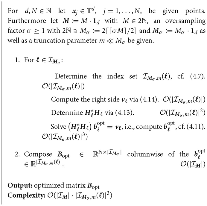
Note that a general statement about the dimensions of $H_{\ell }\in {ℂ}^{\left|{\mathcal{I}}_M\right|\times \left|{\mathcal{I}}_{M_{\sigma },m}(\ell )\right|}$ is not possible, since the size of the set ${\mathcal{I}}_{M_{\sigma },m}(\ell )$ heavily depends on the distribution of the points. To visualize this circumstance, we depicted some exemplary patterns of the nonzero entries of the original matrix $B\in {ℝ}^{N\times \left|{\mathcal{I}}_{M_{\sigma }}\right|}$ in Figure 1. It can easily be seen that for all choices of the points each row contains the same number of nonzero entries, i.e., all index sets (2.12) are of the same size of maximum (2m+1)^d. However, when considering the columns instead, we recognize an evident mismatch in the number of nonzero entries. We remark that because of the fact that each row of $B\in {ℝ}^{N\times \left|{\mathcal{I}}_{M_{\sigma }}\right|}$ contains at most (2m+1)^d entries, each column contains $\frac{N}{\left|{\mathcal{I}}_{M_{\sigma }}\right|}{(2m+1)}^d$ entries on average. A general statement about the maximum size of the index sets (4.7) cannot be made. Roughly speaking, the more irregular the distribution of the points is, the larger the index sets (4.7) can be. Nevertheless, in general $\left|{\mathcal{I}}_{M_{\sigma },m}(\ell )\right|$ is a small constant compared to $\left|{\mathcal{I}}_M\right|$, such that Algorithm 4.3 ends up with total arithmetic costs of approximately $\mathcal{O}(\left|{\mathcal{I}}_M\right|)$.

FIGURE 1

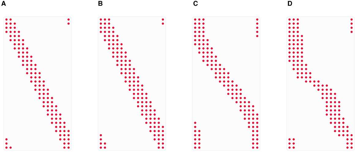
Figure 1. Nonzero entries of the matrix $B\in {ℝ}^{N\times \left|{\mathcal{I}}_{M_{\sigma }}\right|}$ for several choices of the points $x_j\in {𝕋}^d$, j = 1,…, N, with d = 1, M_σ = M = 16, N = 2M, and m = 2. (A) Equispaced points. (B) Jittered points. (C) Chebyshev points. (D) Random points.

In conclusion, our approach for an inverse NFFT can be summarized as follows.

ALGORITHM 4.4

Algorithm 4.4. iNFFT – optimization approach.

Theorem 4.5. Let $B_{\text{opt}}\in {ℝ}^{N\times \left|{\mathcal{I}}_{M_{\sigma }}\right|}$ be the optimized matrix computed by means of Algorithm 4.3 and let $h_{\text{opt}}=D^{*}{F}^{*}{B}_{\text{opt}}^{*}f\in {ℂ}^{\left|{\mathcal{I}}_M\right|}$ be the corresponding approximation of $\widehat{f}$ computed by means of Algorithm 4.4. Further assume that each column $b_{\ell }^{\text{opt}}\in {ℝ}^{\left|{\mathcal{I}}_{M_{\sigma },m}\right|}$ of $B_{\text{opt}}\in {ℝ}^{N\times \left|{\mathcal{I}}_{M_{\sigma }}\right|}$ as solution to (4.10) possesses a small residual

$\begin{array}{ll}\Vert H_{\text{ℓ}}{b}_{\text{ℓ}}^{\text{opt}}-\frac{1}{\left|I_{M_{\text{σ}}}\right|}{D}^{-1}{f}_{\text{ℓ}}{\Vert }_2^2={\epsilon }_{\text{ℓ}}\ge 0,\text{ℓ}\in I_{M_{\text{σ}}}.& (4.15)\end{array}$

Then there exists an ε ≥ 0 such that

$\begin{array}{lll}\Vert h_{\text{opt}}-\widehat{f}{\Vert }_2^2& \le \epsilon {\displaystyle \sum _{k\in I_M}}\frac{1}{\widehat{w}{(k)}^2}·\Vert \widehat{f}{\Vert }_2^2.& (4.16)\end{array}$

Moreover, the (asymmetric) Dirichlet kernel

$\begin{array}{ll}{w}_{\text{D}}:\; ={\displaystyle \sum _{k\in I_M}}{\text{e}}^{2\pi \text{i}kx}={\displaystyle \prod _{t=1}^d}\left(D_{\frac{M}{2}-1}(x_t)+{\text{e}}^{-M\pi \text{i}{x}_t}\right)& (4.17)\end{array}$

is the optimal window function for the inverse NFFT in Algorithm 4.4.

Proof: As in (4.1) the approximation error can be estimated by

$\begin{array}{ll}\begin{array}{l}\begin{array}{l}\Vert h_{opt}-\widehat{f}{\Vert }_2^2=\Vert D^{*}{F}^{*}{B}_{opt}^{*}A-I_{\left|{ℐ}_M\right|}\widehat{F}{\Vert }_2^2\\ \begin{array}{l}\le \Vert D^{*}{F}^{*}{B}_{opt}^{*}A-I_{\left|{ℐ}_M\right|}{\Vert }_{\text{F}}^2\Vert \widehat{F}{\Vert }_2^2.\hfill \end{array}\end{array}\hfill \end{array}& (4.18)\end{array}$

Using the same arguments as for (4.3) and (4.4) we proceed with

$\begin{array}{l}\begin{array}{l}\Vert D^{*}{F}^{*}{B}_{opt}^{*}A-I_{\left|{ℐ}_M\right|}{\Vert }_{\text{F}}^2=\Vert A^{*}{B}_{opt}FD-I_{\left|{ℐ}_M\right|}{\Vert }_{\text{F}}^2\hfill \end{array}\\ \le \Vert A^{*}{B}_{opt}-\frac{1}{\left|I_{M_{\text{σ}}}\right|}{D}^{-1}{F}^{*}{\Vert }_{\text{F}}^2\Vert FD{\Vert }_{\text{F}}^2.& (4.19)\end{array}$

To estimate the first Frobenius norm in (4.19), we rewrite it analogously to (4.8) columnwise as

$\begin{array}{l}\Vert A^{*}{B}_{\text{opt}}-\frac{1}{\Vert I_{M_{\text{σ}}}|}{D}^{-1}{F}^{*}{|}_F^2={\displaystyle \sum _{\text{ℓ}\in I_{M_{\text{σ}}}}}\Vert H_{\text{ℓ}}{b}_{\text{ℓ}}^{\text{opt}}-\frac{1}{\left|I_{M_{\text{σ}}}\right|}{D}^{-1}{f}_{\text{ℓ}}{\Vert }_2^2,\end{array}$

where $b_{\ell }^{\text{opt}}\in {ℝ}^{\left|{\mathcal{I}}_{M_{\sigma },m}(\ell )\right|}$ are the nonzeros of the columns of B_opt, $H_{\ell }\in {ℂ}^{\left|{\mathcal{I}}_M\right|\times \left|{\mathcal{I}}_{M_{\sigma },m}(\ell )\right|}$ in (4.9) are the corresponding submatrices of $A^{*}\in {ℂ}^{\left|{\mathcal{I}}_M\right|\times N}$, cf. (2.7), and $f_{\ell }\in {ℂ}^{\left|{\mathcal{I}}_M\right|}$ are the columns of $F^{*}\in {ℂ}^{\left|{\mathcal{I}}_M\right|\times \left|{\mathcal{I}}_{M_{\sigma }}\right|}$, cf. (2.14). Since $b_{\ell }^{\text{opt}}\in {ℝ}^{\left|{\mathcal{I}}_{M_{\sigma },m}\right|}$ as solutions to the least squares problems (4.10) satisfy (4.15), we can find $\epsilon :=\underset{\ell \in {\mathcal{I}}_{M_{\sigma }}}{max}{\epsilon }_{\ell }\ge 0$, such that ε_ℓ ≤ ε, $\ell \in {\mathcal{I}}_{M_{\sigma }}$, and, therefore,

$\begin{array}{l}{\displaystyle \sum _{\text{ℓ}\in I_{M_{\text{σ}}}}}\Vert H_{\text{ℓ}}{b}_{\text{ℓ}}^{\text{opt}}-\frac{1}{\left|I_{M_{\text{σ}}}\right|}{D}^{-1}{f}_{\text{ℓ}}{\Vert }_2^2\le {\displaystyle \sum _{\text{ℓ}\in I_{M_{\text{σ}}}}}{\epsilon }_{\text{ℓ}}\le \epsilon \left|I_{M_{\text{σ}}}\right|.\end{array}$

Therefore, we may write (4.19) as

$\begin{array}{lll}\Vert D^{*}{F}^{*}{B}_{\text{opt}}^{*}A-I_{\left|I_M\right|}{\Vert }_F^2& \le \epsilon \left|I_{M_{\text{σ}}}\right|·\Vert FD{\Vert }_F^2.& (4.20)\end{array}$

Thus, it remains to estimate the Frobenius norm $\Vert FD{\Vert }_F^2$. By the definitions of the Frobenius norm and the trace tr(Z) of a matrix Z, it is clear that $\left|\right|Z|{|}_F^2=\text{tr}(Z^{*}Z)$. Since by (2.14) we have that $F^{*}F=\left|{\mathcal{I}}_{M_{\sigma }}\right|I_{\left|{\mathcal{I}}_M\right|}$, this yields

$\begin{array}{ll}\Vert FD{\Vert }_F^2=\text{tr}(D^{*}{F}^{*}FD)=\left|I_{M_{\text{σ}}}\right|·\text{tr}(D^{*}D)=\left|I_{M_{\text{σ}}}\right|·\Vert D{\Vert }_F^2.& (4.21)\end{array}$

Using the definition (2.13) of the diagonal matrix $D\in {ℝ}^{\left|{\mathcal{I}}_M\right|\times \left|{\mathcal{I}}_M\right|}$, we obtain

$\begin{array}{ll}\Vert D{\Vert }_F^2=\frac{1}{|I_{M_{\text{σ}}}{|}^2}{\displaystyle \sum _{k\in I_M}}\frac{1}{\widehat{w}{(k)}^2}.& (4.22)\end{array}$

Then combination of (4.20), (4.21), and (4.22) implies

$\begin{array}{ll}\Vert D^{*}{F}^{*}{B}_{\text{opt}}^{*}A-I_{\left|I_M\right|}{\Vert }_F^2& \le \epsilon {\displaystyle \sum _{k\in I_M}}\frac{1}{\widehat{w}{(k)}^2},\end{array}$

such that (4.18) yields the assertion (4.16).

Since it is known that 0 ≤ ŵ(k) ≤ 1, $k\in {\mathcal{I}}_M$, for suitable window functions of the NFFT, cf. [67], we have

$\begin{array}{l}1\le \frac{1}{\widehat{w}(k)}\le \frac{1}{\widehat{w}{(k)}^2}\end{array}$

and, therefore.

$\begin{array}{l}{\displaystyle \sum _{k\in I_M}}\frac{1}{\widehat{w}{(k)}^2}\ge {\displaystyle \sum _{k\in I_M}}1=\left|I_M\right|.\end{array}$

Hence, the smallest constant is achieved in (4.16) when ŵ(k) = 1, $k\in {\mathcal{I}}_M$, i.e., the (asymmetric) Dirichlet kernel (4.17) is the optimal window function for the inverse NFFT in Algorithm 4.4. □

Note that for trigonometric polynomials (2.8) the error bound of Theorem 4.5 with the optimal window function (4.17) is the same as the error bound (3.37) from Theorem 3.14.

Remark 4.6. Up to now, we only focused on the problem (3.4). Finally, considering the inverse adjoint NFFT in (3.5), we remark that this problem can also be solved by means of the optimization procedure in Algorithm 4.3. Assuming again $\left|{\mathcal{I}}_M\right|\le N$, this is the underdetermined setting for the adjoint problem (3.5). Therefore, the minimum norm solution of (3.5) is given by the normal equations of the second kind

$A^{*}Ay=h,f=Ay.$

Incorporating the matrix decomposition of the NFFT, cf. Section 2.1, we recognize that a modification of the matrix $B\in {ℝ}^{N\times \left|{\mathcal{I}}_{M_{\sigma }}\right|}$ such that $A^{*}BFD\approx I_{\left|{\mathcal{I}}_M\right|}$ implies y ≈ h and hence f ≈ BFDh. Thus, the optimization problem (4.3) is also the one to consider for (3.5). In other words, our approach provides both, an inverse NFFT as well as an inverse adjoint NFFT.□

5. Numerics

In conclusion, we have a look at some numerical examples. In addition to comparing the density compensation approach from Section 3 to the optimization approach from Section 4, for both trigonometric polynomials (2.8) and bandlimited functions, we also demonstrate the accuracy of these approaches.

Remark 5.1. At first we introduce some exemplary grids. For visualization we restrict ourselves to the two-dimensional setting d = 2.

(i) We start with a sampling scheme, that is, somehow “close” to the Cartesian grid, but also possesses a random part. To this end, we consider the two-dimensional Cartesian grid and add a two-dimensional perturbation, i.e.,

$\begin{array}{ll}{x}_{t,j}:\; ={\left(-\frac{1}{2}+\frac{2t-1}{N_1},-\frac{1}{2}+\frac{2j-1}{N_2}\right)}^T+{\left(\frac{1}{N_1}{\eta }_1,\frac{1}{N_2}{\eta }_2\right)}^T,& (5.1)\end{array}$

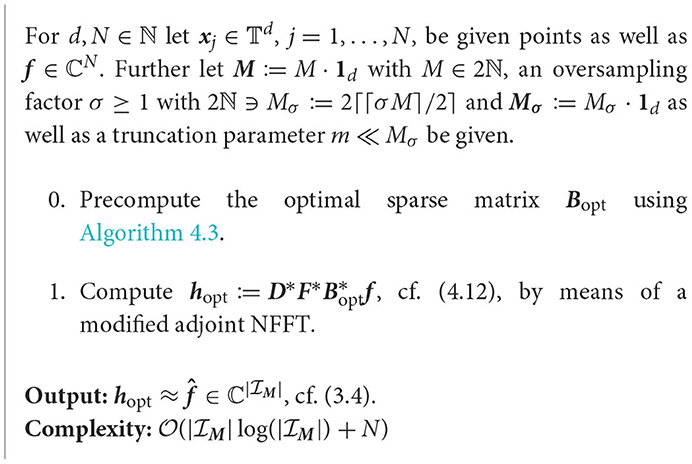
t = 1,…, N₁, j = 1,…, N₂, and η₁, η₂ ~ U(−1, 1), where U(−1, 1) denotes the uniform distribution on the interval (−1, 1). A visualization of this jittered grid can be found in Figure 2A. In addition, we also consider the random grid $x_{t,j}:=\frac{1}{2}{({\eta }_1,{\eta }_2)}^T,$ see Figure 2B.

(ii) Moreover, we examine grids of polar kind, as mentioned in Fenn et al. [68]. For R, T ∈ 2ℕ, the points of the polar grid are given by a signed radius $r_j:=\frac{j}{R}\in \left[-\frac{1}{2},\frac{1}{2}\right)$ and an angle ${\theta }_t:=\frac{\pi t}{T}\in \left[-\frac{\pi }{2},\frac{\pi }{2}\right)$ as

$\begin{array}{ll}{x}_{t,j}:\; =r_j{(cos{\theta }_t,sin{\theta }_t)}^T,{(j,t)}^T\in I_R\times I_T.& (5.2)\end{array}$

Since it is known that the inversion problem is ill-conditioned for this grid we consider a modification, the modified polar grid

$\begin{array}{ll}{x}_{t,j}:\; =r_j{(cos{\theta }_t,sin{\theta }_t)}^T,{(j,t)}^T\in I_{\sqrt{2}R}\times I_T,& (5.3)\end{array}$

i.e., we added more concentric circles and excluded the points outside the unit square, see Figure 3A. Another sampling scheme that is known to lead to more stable results than the polar grid is the linogram or pseudo-polar grid, where the points lie on concentric squares instead of concentric circles, see Figure 3B. There we distinguish two sets of points, i.e.,

$\begin{array}{l}\begin{array}{l}{x}_{t,j}^{BH}:={(\frac{j}{R},\frac{4t}{T}\frac{j}{R})}^T,x_{t,j}^{BV}:={(-\frac{4t}{T}\frac{j}{R},\frac{j}{R})}^T,\hfill \end{array}\\ \begin{array}{l}{(j,t)}^T\in {ℐ}_R\times {ℐ}_{\frac{T}{2}}.\hfill \end{array}& (5.4)\end{array}$

(iii) Another modification of these polar grids was introduced in Helou et al. [69], where the angles θ_t are not chosen equidistantly but are obtained by golden angle increments. For the golden angle polar grid we only exchange the equispaced angles of the polar grid to

$\begin{array}{ll}{\theta }_t=mod\left(\frac{\pi }{2}+t\frac{2\pi }{1+\sqrt{5}},\pi \right)-\frac{\pi }{2},t=0,\dots ,T-1.& (5.5)\end{array}$

The golden angle linogram grid is given by

$\begin{array}{l}{x}_{t,j}:\; =\left\{\begin{array}{cc}{(\frac{2j+1}{2R},\frac{2j+1}{2R}tan({\theta }_t-\frac{\pi }{4}))}^T& :{\theta }_t\in [0,\frac{\pi }{2})\\ {(-\frac{2j+1}{2R}cot({\theta }_t-\frac{\pi }{4}),\frac{2j+1}{2R})}^T& :{\theta }_t\in [-\frac{\pi }{2},0)\\ \end{array}\right\},j\in I_R,\end{array}$

with θ_t in (5.5), as illustrated in Figure 3C.□

FIGURE 2

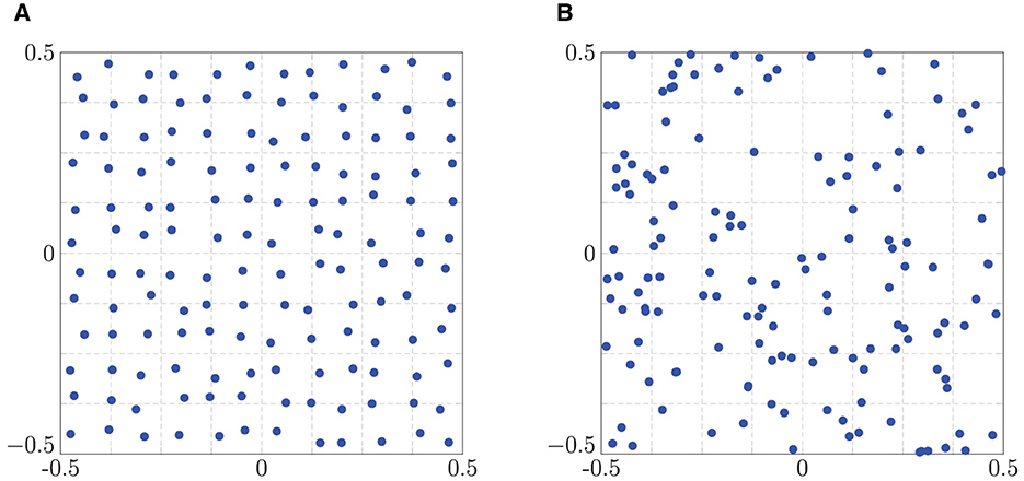
Figure 2. Exemplary randomized grids of size N₁ = N₂ = 12. (A) Jittered grid. (B) Random grid.

FIGURE 3

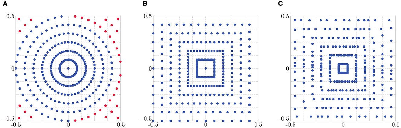
Figure 3. Polar grids of size R = 12 and T = 2R. (A) Polar (blue) and modified polar (red) grid. (B) Linogram/pseudo-polar grid. (C) Golden angle linogram grid.

Before comparing the different approaches from Sections 3 and 4, we study the quality of our methods for the grids mentioned in Remark 5.1. More specifically, in Example 5.2 we investigate the accuracy of the density compensation method from Algorithm 3.7 with the weights introduced in Section 3.1, and in Example 5.3 we check if the norm minimization targeted in Section 4 is successful.

Example 5.2. First, we examine the quality of our density compensation method in Algorithm 3.7 for a trigonometric polynomial f as in (2.8) with given Fourier coefficients ${\widehat{f}}_k\in \left[1,10\right]$, $k\in {\mathcal{I}}_M$. In this test, we consider several d ∈ {1, 2, 3}. For the corresponding function evaluations of (2.8) at given points ${\mathit{x}}_j\in {\left[-\frac{1}{2},\frac{1}{2}\right)}^d$, j = 1,…, N, we test how well these Fourier coefficients can be approximated. More precisely, we consider the estimate ${\tilde{h}}^{\text{w}}=D^{*}{F}^{*}{B}^{*}Wf$, cf. (3.7), with the matrix $W=diag{(w_j)}_{j=1}^N$ of density compensation factors computed by means of Algorithm 3.6, i.e., by (3.15), in case $\left|{\mathcal{I}}_{\mathit{2}\mathit{M}}\right|\le N$, or by (3.16), if $\left|{\mathcal{I}}_{\mathit{2}\mathit{M}}\right|>N$, and compute the relative errors

$\begin{array}{ll}{e}_p:\; =\frac{\Vert {\tilde{h}}^{\text{w}}-\widehat{f}{\Vert }_p}{\Vert \widehat{f}{\Vert }_p},p\in \left\{2,\infty \right\}.& (5.6)\end{array}$

By (3.37), it is known that

$\begin{array}{ll}\frac{\Vert \widehat{f}-A^{*}Wf{\Vert }_p}{\Vert \widehat{f}{\Vert }_p}& \le \left|I_M\right|\epsilon ,p\in \left\{2,\infty \right\},\end{array}$

with the residual $\epsilon =\Vert {\mathit{A}}_{\left|{\mathcal{I}}_{\mathit{2}\mathit{M}}\right|}^T\mathit{w}-{\mathit{e}}_{\mathit{0}}{\Vert }_{\infty }\ge 0$, cf. (3.36).

In our experiment, we use random points x_j with $N_t=2^{9-d}$, t = 1,…, d, cf. Figure 2B, and, for several problem sizes M = M·1_d, M = 2^c with c = 1,…, 11−d, we choose random Fourier coefficients ${\widehat{f}}_k\in \left[1,10\right]$, $k\in {\mathcal{I}}_M$. Afterward, we compute the evaluations of the trigonometric polynomial (2.8) by means of an NFFT and use the resulting vector f as input for the reconstruction. Due to the randomness we repeat this 10 times and then consider the maximum error over all runs. The corresponding results are displayed in Figure 4. It can clearly be seen that $\left|{\mathcal{I}}_{2M}\right|<N$, i.e., as long as $M<\frac{N_1}{2}=2^{8-d}$, the weights computed by means of (3.15) lead to an exact reconstruction of the given Fourier coefficients. However, as soon as we are in the setting $\left|{\mathcal{I}}_{2M}\right|>N$ the least squares approximation via (3.16) does not yield good results anymore.□

FIGURE 4

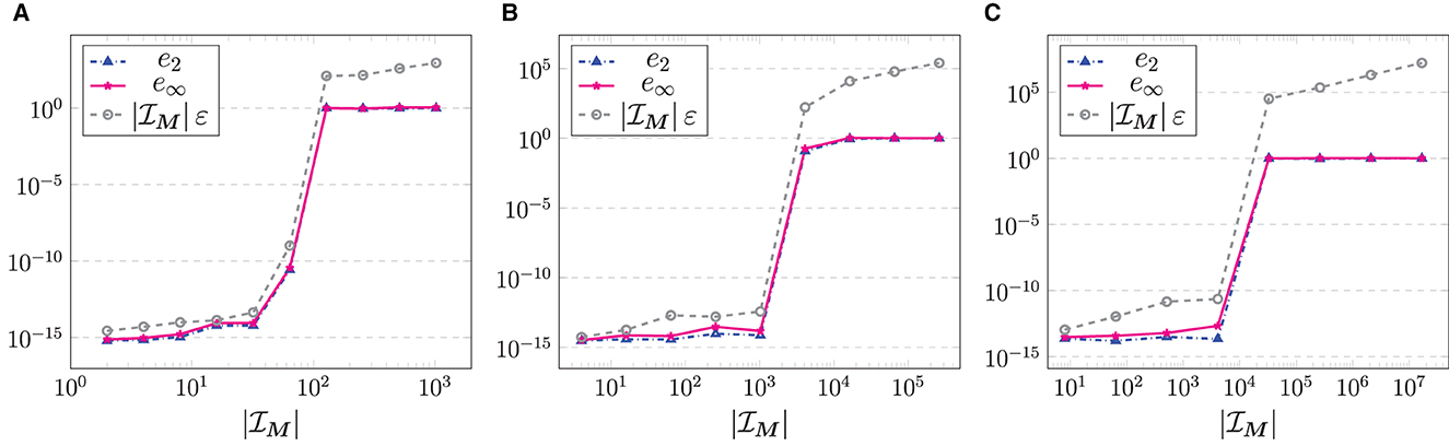
Figure 4. Relative errors (5.6) of the reconstruction of the Fourier coefficients of a trigonometric polynomial (2.8) with given ${\widehat{f}}_k\in \left[1,10\right]$, $k\in {\mathcal{I}}_M$, computed via the density compensation method from Algorithm 3.7, for random grids with $N_t=2^{9-d}$, t = 1,…, d, and M = M·1_d, M = 2^c with c = 1,…, 11−d. (A) d = 1. (B) d = 2. (C) d = 3.

Example 5.3. To study the quality of our optimization method in Section 4, we consider the Frobenius norms

$\begin{array}{c}\begin{array}{c}\hfill n(w,m,\sigma ):=\Vert A^{*}BFD-I_{\left|{ℐ}_M\right|}{\Vert }_{\text{F}},\hfill \end{array}\\ \begin{array}{l}{n}^{opt}(w,m,\sigma ):=\Vert A^{*}{B}_{opt}FD-I_{\left|{ℐ}_M\right|}{\Vert }_{\text{F}},\hfill \end{array}& (5.7)\end{array}$

where B denotes the original matrix from the NFFT in (2.15) and B_opt is the optimized matrix generated by Algorithm 4.3. For the original matrix B we utilize the common B-Spline window function

$\begin{array}{ll}{w}_{\text{B}}:\; =B_{2m}(M_{\text{σ}}x)& (5.8)\end{array}$

with the centered B-Spline of order 2m, cf. [15, p. 388]. The optimized matrix B_opt shall be computed by means of the B-Spline (5.8) as well as the Dirichlet window function (4.17), which is the optimal window by Theorem 4.5.

Due to memory limitations in the computation of the Frobenius norms (5.7), we have to settle for very small problems, which however show the functionality of Algorithm 4.3. For this reason, we consider d = 2 and choose M = (12, 12)^T as well as $N_1=N_2=R=2^{\mu }$, μ ∈ {2,…, 7}, and T = 2R for the grids mentioned in Remark 5.1. In other words, we test Algorithm 4.3 in the underdetermined setting $\left|{\mathcal{I}}_M\right|>N$ as well as for the overdetermined setting $\left|{\mathcal{I}}_M\right|\le N$.

Having a look at the results for the grids in Remark 5.1, it becomes apparent that they separate into two groups. Figure 5A displays the results for the polar grid (5.2), which are the same as for the golden angle polar grid, cf. (5.5). In these cases there is only a slight improvement by the optimization. However, for all other mentioned grids the minimization procedure in Algorithm 4.3 is very effective. The results of these grids are depicted in Figure 5B exemplarily for the modified polar grid (5.3). Moreover, it can be seen that our optimization procedure in Algorithm 4.3 is the most effective in the overdetermined setting $\left|{\mathcal{I}}_M\right|\le N$.

FIGURE 5

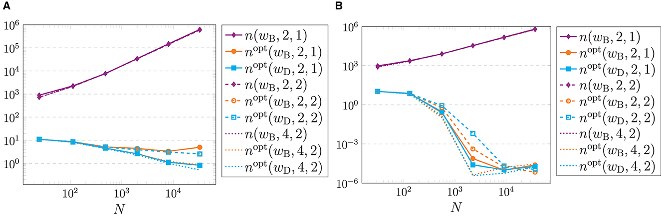
Figure 5. Frobenius norms (5.7) of the original matrix B (violet) and the optimized matrix B_opt generated by Algorithm 4.3 using the B-Spline w_B (orange) as well as the Dirichlet window w_D (cyan) with R = 2^μ, μ ∈ {2,…, 7}, and T = 2R as well as M = (12, 12)^T, m ∈ {2, 4}, and σ ∈ {1, 2}. (A) Polar grid (5.2). (B) Modified polar grid (5.3).

One reason for the different behavior of polar and modified polar grid could be the ill-posedness of the inversion problem for the polar grid, which becomes evident in huge condition numbers of $H_{\ell }^{*}{H}_{\ell }$, whereas the problem for modified polar grids is well-posed. Another reason can be found in the optimization procedure itself. Having a closer look at the polar grid, see Figure 3A, there are no grid points in the corners of the unit square. Therefore, some of the index sets ${\mathcal{I}}_{M_{\sigma },m}(\ell )$, cf. (4.7), are empty and no optimization can be done for the corresponding matrix columns. This could also cause the worsened minimization properties of the polar grid.□

Next, we proceed with comparing the density compensation approach from Section 3 using the weights w_j introduced in Section 3.1 to the optimization approach for modifying the matrix B from Section 4. To this end, we show an example concerning trigonometric polynomials (2.8) of degree M and a second one that deals with bandlimited functions of bandwidth M. Here, we restrict ourselves to the two-dimensional setting d = 2 for better visualization of the results.

Example 5.4. Similar to Averbuch et al. [32] and Kircheis and Potts [33] we have a look at the reconstruction of the Shepp-Logan phantom, see Figure 6A. Here, we treat the phantom data as given Fourier coefficients $\widehat{f}:={({\widehat{f}}_k)}_{k\in {\mathcal{I}}_M}$ of a trigonometric polynomial (2.8). For given points ${\mathit{x}}_j\in {\left[-\frac{1}{2},\frac{1}{2}\right)}^d$, j = 1,…, N, we then compute the evaluations of the trigonometric polynomial (2.8) by means of an NFFT and use the resulting vector as input for the reconstruction.

FIGURE 6

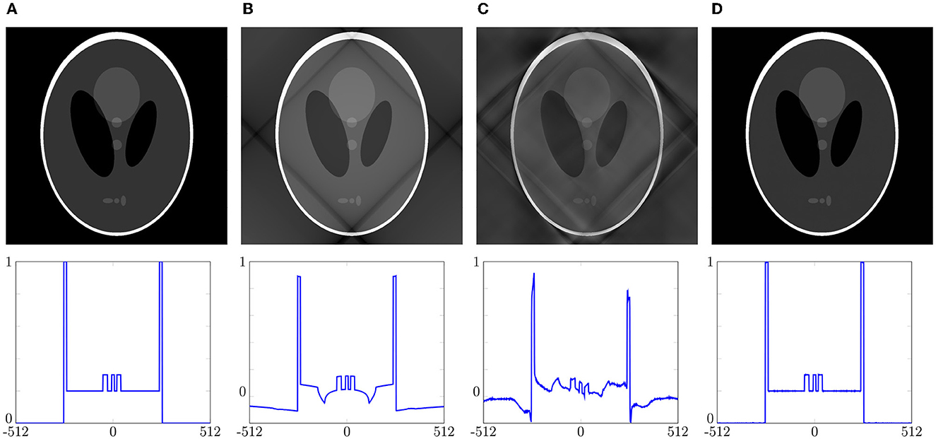
Figure 6. Reconstruction of the Shepp-Logan phantom of size 1024 × 1024 (top) via the density compensation method from Section 3.1 using Voronoi weights and Algorithm 3.7 with weights computed by (3.16) compared to Algorithm 4.4 for the linogram grid (5.4) of size R = M = 1, 024, T = 2R; as well as a detailed view of the 832nd row each (bottom). (A) Original phantom. (B) Voronoi weights with e₂=5.3040e-01. (C) Algorithm 3.7 with e₂=5.0585e-01. (D) Algorithm 4.4 with e₂=2.2737e-03.

In a first experiment, we test the inversion methods from Sections 3 and 4 as in Averbuch et al. [32] for increasing input sizes. To this end, we choose M = (M, M)^T, M = 2^c with c = 3,…, 10, and linogram grids (5.4) of size R = 2M, T = 2R, i.e., we consider the setting $\left|{\mathcal{I}}_{2M}\right|<N$. For using Algorithm 4.4 we choose the oversampling factor σ = 1.0 and the truncation parameter m = 4. For each input size we measure the computation time of the precomputational steps, i.e., the computation of the weight matrix W or the computation of the optimized sparse matrix B_opt, as well as the time needed for the reconstruction, i.e., the corresponding adjoint NFFT, see Algorithms 3.7, 4.4. Moreover, for the reconstruction $\tilde{h}\in \left\{{\tilde{h}}^{\text{w}},h_{\text{opt}}\right\}$, cf. (3.7) and (4.12), we consider the relative errors

$\begin{array}{ll}{e}_2:\; =\frac{\Vert \tilde{h}-\widehat{f}{\Vert }_2}{\Vert \widehat{f}{\Vert }_2}.& (5.9)\end{array}$

The corresponding results can be found in Table 1. We remark that since we are in the setting $\left|{\mathcal{I}}_{2M}\right|<N$, the density compensation method in Algorithm 3.7 with weights computed by (3.15) indeed produces nearly exact results. Although, our optimization procedure from Algorithm 4.4 achieves small errors as well, this reconstruction is not as good as the one by means of our density compensation method.

TABLE 1

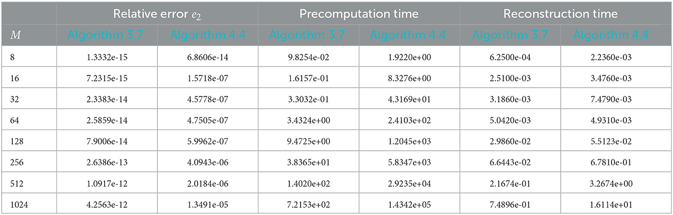
Table 1. Relative errors (5.9) of the reconstruction of the Shepp-Logan phantom of size M as well as the runtime in seconds for the density compensation method from Algorithm 3.7 compared to Algorithm 4.4 with σ = 1.0 and m = 4, using linogram grids (5.4) of size R = 2M, T = 2R.

Note that in comparison to Averbuch et al. [32], our method in Algorithm 3.7 using density compensation produces errors of the same order, but is much more effective for solving several problems using the same points x_j for different input values f. Since our precomputations have to be done only once in this setting, we strongly profit from the fact that we only need to perform an adjoint NFFT as reconstruction, which is very fast, whereas in Averbuch et al. [32] they would need to execute their whole routine each time again.

As a second experiment, we aimed to decrease the amount of overdetermination, i.e., we want to keep the size $\left|{\mathcal{I}}_M\right|$ of the phantom, but reduce the number N of the points x_j, j = 1,…, N. To this end, we now consider linogram grids (5.4) of the smaller size R = M, T = 2R, i.e., now we have $\left|{\mathcal{I}}_{2M}\right|>N$.

The reconstruction of the phantom of size 1, 024 × 1, 024 is presented in Figure 6 (top) including a detailed view of the 832nd row of this reconstruction (bottom). Despite the reconstruction via Algorithm 4.4 as well as the density compensation method using weights computed by means of (3.16), we also considered the result using Voronoi weights. For all approaches we added the corresponding relative errors (5.9) to Figure 6 as well.

Due to the fact that the exactness condition $\left|{\mathcal{I}}_{2M}\right|<N$ (cf. Section 3.1.1) is violated, it can be seen in Figure 6C that the density compensation method using weights computed by means of (3.16) does not yield an exact reconstruction is this setting. On the contrary, we recognize that our optimization method, see Figure 6D, achieves a huge improvement in comparison to the density compensation techniques in Figures 6B, C since no artifacts are visible. Presumably, this arises because there are more degrees of freedom in the optimization of the matrix B from Section 4 than with the density compensation techniques from Section 3, cf. Remark 3.1. We remark that although the errors are not as small as in Table 1, by comparing Figures 6A, D and it becomes apparent that the differences are not even visible anymore. Note that for this result the number N of points is ca. four times lower as for the results depicted in Table 1, i.e., we only needed twice as much function values as Fourier coefficients, whereas e.g., in [32] they worked with a factor of more than 4.□

Example 5.5. Finally, we examine the reconstruction properties for bandlimited functions $f\in L_1({ℝ}^d)\cap C_0({ℝ}^d)$ with maximum bandwidth M. To this end, we first specify a compactly supported function $\widehat{f}$ and consequently compute its inverse Fourier transform f, such that its samples f(x_j) for given ${\mathit{x}}_j\in {\left[-\frac{1}{2},\frac{1}{2}\right)}^d$, j = 1, …, N, can be used for the reconstruction of the samples $\widehat{f}(k)$, $k\in {\mathcal{I}}_M$. Here, we consider the tensorized function $\widehat{f}(v)=g(v_1)·g(v_2)$, where g(v) is the one-dimensional triangular pulse $g(v):=(1-\left|\frac{v}{b}\right|)·{\chi }_{\left[-b,b\right]}(v)$. Then for all b ∈ ℕ with $b\le \frac{M}{2}$ the associated inverse Fourier transform

$\begin{array}{l}f(x)=\underset{{ℝ}^2}{{{\displaystyle \int }}^{\text{}}}\widehat{f}(v){\text{e}}^{2\pi \text{i}vx}dv=b^{2}sin{c}^2(b\pi x)\hfill \\ =b^{2}sin{c}^2(b\pi x_1)sin{c}^2(b\pi x_2),x\in {ℝ}^2,\hfill \end{array}$

is bandlimited with bandwidth M. In this case, we consider M = 64 and b = 24 as well as the jittered grid (5.1) of size N₁ = N₂ = 144, i.e., we study the setting $\left|{\mathcal{I}}_{\mathit{2}\mathit{M}}\right|\le N$.

Now, the aim was to compare the different density compensation methods considered in Section 3 and the optimization approach from Section 4. More precisely, we consider the reconstruction using Voronoi weights, the weights computed via (3.58), the weights in (3.62), and Algorithm 3.7 with weights computed via (3.15), as well as Algorithm 4.4. For the reconstruction $\tilde{h}\in \left\{{\tilde{h}}^{\text{w}},h_{\text{opt}}\right\}$, cf. (3.7) and (4.12), we then compute the pointwise absolute errors $\tilde{h}-\widehat{f}$. The corresponding results are displayed in Figure 7. It can easily be seen that Voronoi weights, see Figure 7A, and the weights in (3.62), see Figure 7D, do not yield a good reconstruction, as expected. The other three approaches produce nearly the same reconstruction error, which is also obtained by reconstruction on an equispaced grid and, therefore, is the best possible. In other words, in case of bandlimited functions the truncation error in (3.20) is dominating and thus reconstruction errors smaller than the ones shown in Figure 7 cannot be expected.

FIGURE 7

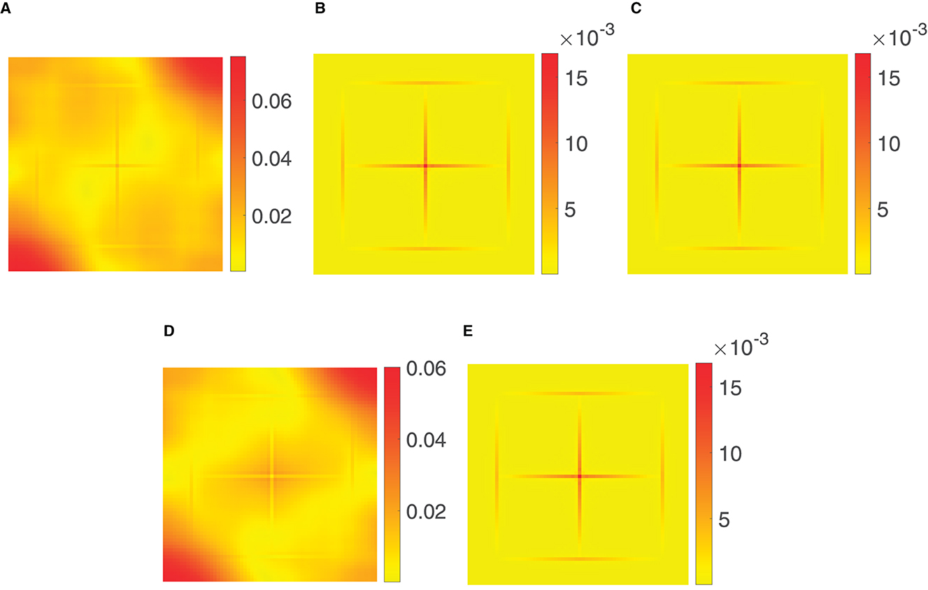
Figure 7. Pointwise absolute error $\left|\tilde{h}-\widehat{f}\right|$ of the reconstruction of samples $\widehat{f}(k)$ of the tensorized triangular pulse function with M = 64 and b = 24, using the density compensation methods considered in Section 3 as well as the optimization approach from Algorithm 4.4 for the jittered grid (5.1) of size N₁ = N₂ = 144. (A) Voronoi weights. (B) Algorithm 3.7. (C) Weights via (3.58). (D) Weights (3.62). (E) Algorithm 4.4.

Note that the comparatively small choice of M = 64 was made in order that the computation of the weights via (3.58), see Figure 7C, as well as the weights in (3.62), see Figure 7D, is affordable, cf. Section 3.4.2. In contrast, our new methods using Algorithm 3.7, see Figure 7B, or Algorithm 4.4, see Figure 7E, are much more effective and, therefore, better suited for the given problem.

6. Conclusion

In the present article, we considered several direct methods for computing an inverse NFFT, i.e., reconstructing the Fourier coefficients ${\widehat{f}}_k$, $k\in {\mathcal{I}}_M$, from given nonequispaced data f(x_j), j = 1,…, N. Being a direct method here means, that for a fixed set of points x_j, j = 1,…, N, the reconstruction can be realized with the same number of arithmetic operations as a single application of an adjoint NFFT (see Algorithm 2.4). As we have seen in (3.3), a certain precomputational step is compulsory, since the adjoint NFFT does not yield an inversion by itself. Although this precomputations might be rather costly, they need to be done only once for a given set of points x_j, j = 1,…, N. Therefore, direct methods are especially beneficial in case of fixed points. For this reason, we studied two different approaches of this kind and especially focused on methods for the multidimensional setting d ≥ 1 that are applicable to general sampling patterns.

First, in Section 3, we examined the well-known approach of sampling density compensation, where suitable weights w_j ∈ ℂ, j = 1,…, N, are precomputed, such that the reconstruction can be realized by means of an adjoint NFFT applied to the scaled data w_jf(x_j). We started our investigations with trigonometric polynomials in Section 3.1. In Corollary 3.4, we introduced the main formula (3.14), which yields exact reconstruction for all trigonometric polynomials of degree M. In addition to this theoretical considerations, we also discussed practical computation schemes for the overdetermined as well as the underdetermined setting, as summarized in Algorithm 3.6. Afterward, in Section 3.2, we studied the case of bandlimited functions, which often occurs in the context of MRI and discussed that the same numerical procedures as in Section 3.1 can be used in this setting as well. In Section 3.3, we then summarized the previous findings by presenting a general error bound on density compensation factors computed by means of Algorithm 3.6 in Theorem 3.14. In addition, this also yields an estimate on the condition number of the matrix product A^*WA, as shown in Theorem 3.15. In Section 3.4, we surveyed certain approaches from literature and commented on their connection among each other as well as to the method presented in Section 3.1.

Subsequently, in Section 4, we studied another direct inversion method, where the matrix representation A ≈ BFD of the NFFT is used to modify the sparse matrix B, such that a reconstruction is given by $\widehat{f}{D}^{*}{F}^{*}{B}_{opt}^{*}f$. In other words, the inversion is done by a modified adjoint NFFT, while the optimization of the matrix B can be realized in a precomputational step, see Algorithm 4.4.

Finally, in Section 5, we had a look at some numerical examples to investigate the accuracy of the previously introduced methods. We have seen that our approaches are best-suited for the overdetermined setting $\left|{\mathcal{I}}_M\right|\le N$ and work for many different sampling patterns. More specifically, in the highly overdetermined case $\left|{\mathcal{I}}_{2M}\right|\le N$ we have theoretically proven as well as numerically verified in several examples that the density compensation technique in Algorithm 3.7 leads to an exact reconstruction for trigonometric polynomials. In case not that much data are available and we have to reduce the amount of overdetermination such that $\left|{\mathcal{I}}_{2M}\right|>N$, we have shown that the optimization approach from Algorithm 4.4 is preferable, since the higher number of degrees of freedom in the optimization (see Remark 3.1) yields better results. In addition, also for the setting of bandlimited functions we demonstrated that our methods are much more efficient than existing ones.

Data availability statement

The original contributions presented in the study are included in the article/supplementary material, further inquiries can be directed to the corresponding author.

Author contributions

All authors listed have made a substantial, direct, and intellectual contribution to the work and approved it for publication.

Funding

MK gratefully acknowledges the support from the BMBF grant 01∣S20053A (project SAℓE). DP acknowledges the funding by Deutsche Forschungsgemeinschaft (German Research Foundation) – Project–ID 416228727 – SFB 1410.

Acknowledgments

The authors thank the referees and the editor for their very useful suggestions for improvements.

Conflict of interest

The authors declare that the research was conducted in the absence of any commercial or financial relationships that could be construed as a potential conflict of interest.

Publisher's note

All claims expressed in this article are solely those of the authors and do not necessarily represent those of their affiliated organizations, or those of the publisher, the editors and the reviewers. Any product that may be evaluated in this article, or claim that may be made by its manufacturer, is not guaranteed or endorsed by the publisher.

References

1. Doneva M, Akcakaya M, Prieto C, editors. Magnetic Resonance Image Reconstruction: Theory, Methods and Applications, Volume 6. Cambridge, MA: Academic Press (2022).

2. Eggers H, Kircheis M, Potts D. on-Cartesian MRI reconstruction. In:Doneva M, Akcakaya M, Prieto C, , editors. Magnetic Resonance Image Reconstruction: Theory, Methods and Applications, Volume 6. Cambridge, MA: Academic Press (2022). doi: 10.1016/B978-0-12-822726-8.00013-0

CrossRef Full Text | Google Scholar

3. Fasshauer GE. Meshfree Approximation Methods with MATLAB. Singapore: World Scientific Publishers (2007). doi: 10.1142/6437

CrossRef Full Text | Google Scholar

4. Feichtinger HG, Gröchenig K, Strohmer T. Efficient numerical methods in non-uniform sampling theory. Numer Math. (1995) 69:423–40. doi: 10.1007/s002110050101

PubMed Abstract | CrossRef Full Text | Google Scholar

5. Bass RF, Gröchenig K. Random sampling of multivariate trigonometric polynomials. SIAM J Math Anal. (2004) 36:773–95. doi: 10.1137/S0036141003432316

CrossRef Full Text | Google Scholar

6. Böttcher A, Potts D. Probability against condition number and sampling of multivariate trigonometric random polynomials. Electron Trans Numer Anal. (2007) 26:178–189.

Google Scholar

7. Kunis S, Potts D. Time and memory requirements of the nonequispaced FFT. Sampl Theory Signal Image Process. (2008) 7:77–100. doi: 10.1007/BF03549487

CrossRef Full Text | Google Scholar

8. Kunis S, Nagel D. On the condition number of Vandermonde matrices with pairs of nearly-colliding nodes. Numer Algor. (2021) 87:473–96. doi: 10.1007/s11075-020-00974-x

CrossRef Full Text | Google Scholar

9. Ruiz-Antolin D, Townsend A. A nonuniform fast Fourier transform based on low rank approximation. SIAM J Sci Comput. (2018) 40:A529–47. doi: 10.1137/17M1134822

CrossRef Full Text | Google Scholar

10. Sutton BP, Fessler JA, Noll DC. A min-max approach to the nonuniform N-dimensional FFT for rapid iterative reconstruction of MR images. In: Proceedings of the 9th Annual Meeting of the International Society for Magnetic Resonance in Medicine. Scotland (2001). p. 763.

Google Scholar

11. Fessler JA, Sutton BP. Nonuniform fast Fourier transforms using min-max interpolation. IEEE Trans Signal Process. (2003) 51:560–74. doi: 10.1109/TSP.2002.807005

CrossRef Full Text | Google Scholar

12. Knopp T, Kunis S, Potts D. A note on the iterative MRI reconstruction from nonuniform k-space data. Int J Biomed Imag. (2007) 2007:24727. doi: 10.1155/2007/24727

PubMed Abstract | CrossRef Full Text | Google Scholar

13. Pruessmann KP, Wayer FTAW. Major speedup of reconstruction for sensitivity encoding with arbitrary trajectories. In: Proc. Intl. Soc. Mag. Reson. Med. 9. Glasgow (2001), p. 767.

14. Kunis S, Potts D. Stability results for scattered data interpolation by trigonometric polynomials. SIAM J Sci Comput. (2007) 29:1403–19. doi: 10.1137/060665075

CrossRef Full Text | Google Scholar

15. Plonka G, Potts D, Steidl G, Tasche M. Numerical Fourier Analysis. Applied and Numerical Harmonic Analysis. Boston, MA: Birkhäuser (2018). doi: 10.1007/978-3-030-04306-3

PubMed Abstract | CrossRef Full Text | Google Scholar

16. Stefan W, Renaut RA, Gelb A. Improved total variation-type regularization using higher order edge detectors. SIIMS. (2010) 3:232–51. doi: 10.1137/080730251

CrossRef Full Text | Google Scholar

17. Wasserman G, Archibald R, Gelb A. Image reconstruction from Fourier data using sparsity of edges. J Sci Comput. (2015) 65:533–52. doi: 10.1007/s10915-014-9973-3

CrossRef Full Text | Google Scholar

18. Archibald R, Gelb A, Platte RB. Image reconstruction from undersampled Fourier data using the polynomial annihilation transform. J Sci Comput. (2016) 67:432–52. doi: 10.1007/s10915-015-0088-2

CrossRef Full Text | Google Scholar

19. Archibald R, Gelb A, Yoon J. Polynomial fitting for edge detection in irregularly sampled signals and images. SINUM. (2005) 43:259–79. doi: 10.1137/S0036142903435259

CrossRef Full Text | Google Scholar

20. Candès EJ, Wakin MB, Boyd SP. Enhancing sparsity by reweighted ℓ₁ minimization. J Fourier Anal Appl. (2008) 14:877–905. doi: 10.1007/s00041-008-9045-x

CrossRef Full Text | Google Scholar

21. Chartrand R, Yin W. Iteratively reweighted algorithms for compressive sensing. In: IEEE International Conference on Acoustics, Speech and Signal Processing. Las Vegas, NV: IEEE (2008), p. 3869–72. doi: 10.1109/ICASSP.2008.4518498

CrossRef Full Text | Google Scholar

22. Daubechies I, DeVore R, Fornasier M, Güntürk CS. Iteratively reweighted least squares minimization for sparse recovery. Commun Pure Appl Math. (2010) 63:1–38. doi: 10.1002/cpa.20303

PubMed Abstract | CrossRef Full Text | Google Scholar

23. Liu Y, Ma J, Fan Y, Liang Z. Adaptive-weighted total variation minimization for sparse data toward low-dose X-ray computed tomography image reconstruction. Phys Med Biol. (2012) 57:7923. doi: 10.1088/0031-9155/57/23/7923

PubMed Abstract | CrossRef Full Text | Google Scholar

24. Churchill V, Archibald R, Gelb A. Edge-adaptive ℓ₂ regularization image reconstruction from non-uniform Fourier data. Inverse Probl Imaging. (2019) 13:931–58. doi: 10.3934/ipi.2019042

CrossRef Full Text | Google Scholar

25. Scarnati T, Gelb A. Accelerated variance based joint sparsity recovery of images from Fourier data. arXiv. (2019). doi: 10.48550/arXiv.1910.08391

CrossRef Full Text | Google Scholar

26. Dutt A, Rokhlin V. Fast Fourier transforms for nonequispaced data II. Appl Comput Harmon Anal. (1995) 2:85–100. doi: 10.1006/acha.1995.1007

CrossRef Full Text | Google Scholar

27. Selva J. Efficient type-4 and type-5 non-uniform FFT methods in the one-dimensional case. IET Signal Process. (2018) 12:74–81. doi: 10.1049/iet-spr.2016.0509

CrossRef Full Text | Google Scholar

28. Kircheis M, Potts D. Direct inversion of the nonequispaced fast Fourier transform. Linear Algebra Appl. (2019) 575:106–40. doi: 10.1016/j.laa.2019.03.028

CrossRef Full Text | Google Scholar

29. Heinig G, Rost K. Algebraic Methods for Toeplitz-like Matrices and Operators, Volume 19 of Mathematical Research. Berlin: Akademie-Verlag (1984). doi: 10.1515/9783112529003

CrossRef Full Text | Google Scholar

30. Gelb A, Song G. A frame theoretic approach to the nonuniform fast Fourier transform. SIAM J Numer Anal. (2014) 52:1222–42. doi: 10.1137/13092160X

CrossRef Full Text | Google Scholar

31. Averbuch A, Coifman R, Donoho DL, Elad M, Israeli M. Fast and accurate polar Fourier transform. Appl Comput Harmon Anal. (2006) 21:145–67. doi: 10.1016/j.acha.2005.11.003

CrossRef Full Text | Google Scholar

32. Averbuch A, Coifman R, Donoho D, Israeli M, Shkolnisky Y. A framework for discrete integral transformations I—the pseudopolar Fourier transform. SIAM J Sci Comput. (2008) 30:764–84. doi: 10.1137/060650283

CrossRef Full Text | Google Scholar

33. Kircheis M, Potts D. Efficient multivariate inversion of the nonequispaced fast Fourier transform. PAMM. (2021) 20:e202000120. doi: 10.1002/pamm.202000120

CrossRef Full Text | Google Scholar

34. Dutt A, Rokhlin V. Fast Fourier transforms for nonequispaced data. SIAM J Sci Stat Comput. (1993) 14:1368–93. doi: 10.1137/0914081

CrossRef Full Text | Google Scholar

35. Beylkin G. On the fast Fourier transform of functions with singularities. Appl Comput Harmon Anal. (1995) 2:363–81. doi: 10.1006/acha.1995.1026

CrossRef Full Text | Google Scholar

36. Steidl G. A note on fast Fourier transforms for nonequispaced grids. Adv Comput Math. (1998) 9:337–53.

Google Scholar

37. Greengard L, Lee J-Y. Accelerating the nonuniform fast Fourier transform. SIAM Rev. (2004) 46:443–54. doi: 10.1137/S003614450343200X

CrossRef Full Text | Google Scholar

38. Keiner J, Kunis S, Potts D. Using NFFT 3 – a software library for various nonequispaced fast Fourier transforms. ACM Trans Math Softw. (2009) 36:1–30. Available online at: https://www.researchgate.net/publication/220492570_Using_NFFT_3—A_Software_Library_for_Various_Nonequispaced_Fast_Fourier_Transforms

Google Scholar

39. Duijndam AJW, Schonewille MA. Nonuniform fast Fourier transform. Geophysics. (1999) 64:539–51. doi: 10.1190/1.1444560

CrossRef Full Text | Google Scholar

40. Fourmont K. Non equispaced fast Fourier transforms with applications to tomography. J Fourier Anal Appl. (2003) 9:431–50. doi: 10.1007/s00041-003-0021-1

CrossRef Full Text | Google Scholar

41. Potts D, Tasche M. Continuous window functions for NFFT. Adv Comput Math. (2021) 47:1–34. doi: 10.1007/s10444-021-09873-8

CrossRef Full Text | Google Scholar

42. Keiner J, Kunis S, Potts D. NFFT 3.5, C subroutine library. https://www.tu-chemnitz.de/~potts/nfft/. Contributors: Bartel F, Fenn M, Görner T, Kircheis M, Knopp T, Quellmalz M, Schmischke M, Volkmer T, and Vollrath A.

Google Scholar

43. Rasche V Proksa R Sinkus R Börnert P and Eggers H. Resampling of data between arbitrary grids using convolution interpolation. IEEE Trans Med Imag. (1999) 18:385–92. doi: 10.1109/42.774166

PubMed Abstract | CrossRef Full Text | Google Scholar

44. Gräf M, Kunis S, Potts D. On the computation of nonnegative quadrature weights on the sphere. Appl Comput Harmon Anal. (2009) 27:124–32. doi: 10.1016/j.acha.2008.12.003

CrossRef Full Text | Google Scholar

45. Tchakaloff V. Formules de cubature mécaniques à coefficients non négatifs. Bull Sci Math. (1957) 81:123–34.

Google Scholar

46. Gröchenig K. Sampling, Marcinkiewicz-Zygmund inequalities, approximation, and quadrature rules. J Approx Theory. (2020) 257:105455. doi: 10.1016/j.jat.2020.105455

CrossRef Full Text | Google Scholar

47. Huybrechs D. Stable high-order quadrature rules with equidistant points. J Comput Appl Math. (2009) 231:933–47. doi: 10.1016/j.cam.2009.05.018

CrossRef Full Text | Google Scholar

48. Whittaker ET. On the functions which are represented by the expansions of the interpolation theory. Proc R Soc Edinb. (1915) 35:181–94. doi: 10.1017/S0370164600017806

CrossRef Full Text | Google Scholar

49. Shannon CE. Communication in the presence of noise. Proc IRE. (1949) 37:10–21. doi: 10.1109/JRPROC.1949.232969

CrossRef Full Text | Google Scholar

50. Kotelnikov VA. On the transmission capacity of the “ether” and wire in electrocommunications. In:Benedetto JJ, Ferreira JSG, , editors. Modern Sampling Theory: Mathematics and Application. Boston, MA: Birkhäuser (2001), p. 27–45. Translated from Russian. doi: 10.1007/978-1-4612-0143-4_2

CrossRef Full Text | Google Scholar

51. Qian L. On the regularized Whittaker-Kotelnikov-Shannon sampling formula. Proc Amer Math Soc. (2003) 131:1169–76. doi: 10.1090/S0002-9939-02-06887-9

CrossRef Full Text | Google Scholar

52. Strohmer T, Tanner J. Fast reconstruction methods for bandlimited functions from periodic nonuniform sampling. SIAM J Numer Anal. (2006) 44:1071–94. doi: 10.1137/040609586

CrossRef Full Text | Google Scholar

53. Micchelli C, Xu Y, Zhang H. Optimal learning of bandlimited functions from localized sampling. J Complexity. (2009) 25:85–114. doi: 10.1016/j.jco.2009.02.005

PubMed Abstract | CrossRef Full Text | Google Scholar

54. Lin R, Zhang H. Convergence analysis of the Gaussian regularized Shannon sampling formula. Numer Funct Anal Optim. (2017) 38:224–47. doi: 10.1080/01630563.2016.1240182

CrossRef Full Text | Google Scholar

55. Kircheis M, Potts D, Tasche M. On regularized Shannon sampling formulas with localized sampling. Sampl Theory Signal Process Data Anal. (2022) 20:20. doi: 10.1007/s43670-022-00039-1

CrossRef Full Text | Google Scholar

56. Kircheis M, Potts D, Tasche M. Nonuniform fast Fourier transforms with nonequispaced spatial and frequency data and fast sinc transforms. Numer Algor92. (2022) 2307–39. doi: 10.1007/s11075-022-01389-6

CrossRef Full Text | Google Scholar

57. Elbel B, Steidl G. Fast Fourier transform for nonequispaced data. In:Chui CK, Schumaker LL, , editors. Approximation Theory IX. Nashville: Vanderbilt University Press (1998), p. 39–46.

Google Scholar

58. Lee J-Y, Greengard L. The type 3 nonuniform FFT and its applications. J Comput Phys. (2005) 206:1–5. doi: 10.1016/j.jcp.2004.12.004

CrossRef Full Text | Google Scholar

59. Gopal A, Rokhlin V. A fast procedure for the construction of quadrature formulas for bandlimited functions. Technical Report, YALEU/DCS/TR-1563. (2022). doi: 10.1016/j.acha.2023.05.001

CrossRef Full Text | Google Scholar

60. Björck Å. Numerical Methods for Least Squares Problems. Philadelphia, PA: SIAM (1996). doi: 10.1137/1.9781611971484

CrossRef Full Text | Google Scholar

61. Sedarat H, Nishimura DG. On the optimality of the gridding reconstruction algorithm. IEEE Trans Med Imaging. (2000) 19:306–17. doi: 10.1109/42.848182

PubMed Abstract | CrossRef Full Text | Google Scholar

62. Rosenfeld D. An optimal and efficient new gridding algorithm using singular value decomposition. Magn Reson Med. (1998) 40:14–23. doi: 10.1002/mrm.1910400103

PubMed Abstract | CrossRef Full Text | Google Scholar

63. Pipe JG, Menon P. Sampling density compensation in MRI: rationale and an iterative numerical solution. Magn Reson Med. (1999) 41:179–86. doi: 10.1002/(SICI)1522-2594(199901)41:1<179::AID-MRM25>3.0.CO;2-V

PubMed Abstract | CrossRef Full Text | Google Scholar

64. Choi H, Munson DC. Analysis and design of minimax-optimal interpolators. IEEE Trans Signal Process. (1998) 46:1571–9. doi: 10.1109/78.678470

CrossRef Full Text | Google Scholar

65. Greengard L, Lee J-Y, Inati S. The fast sinc transform and image reconstruction from nonuniform samples in k-space. Commun Appl Math Comput Sci. (2006) 1:121–31. doi: 10.2140/camcos.2006.1.121

CrossRef Full Text | Google Scholar

66. Nieslony A, Steidl G. Approximate factorizations of Fourier matrices with nonequispaced knots. Linear Algebra Appl. (2003) 266:337–51. doi: 10.1016/S0024-3795(02)00496-2

CrossRef Full Text | Google Scholar

67. Potts D, Tasche M. Uniform error estimates for nonequispaced fast Fourier transforms. Sampl Theory Signal Process Data Anal. (2021) 19:1–42. doi: 10.1007/s43670-021-00017-z

CrossRef Full Text | Google Scholar

68. Fenn M, Kunis S, Potts D. On the computation of the polar FFT. Appl Comput Harmon Anal. (2007) 22:257–63. doi: 10.1016/j.acha.2006.05.009

CrossRef Full Text | Google Scholar

69. Helou ES, Zibetti MVW, Axel L, Block KT, Regatte RR, Herman GT. The discrete Fourier transform for golden angle linogram sampling. Inverse Probl. (2019) 35:125004. doi: 10.1088/1361-6420/ab44ee

CrossRef Full Text | Google Scholar

70. Stewart G. Matrix Algorithms: Basic Decompositions. Philadelphia, PA: SIAM (1998). doi: 10.1137/1.9781611971408

CrossRef Full Text | Google Scholar

71. Lund J, Bowers KL. Sinc Methods for Quadrature and Differential Equations. Philadelphia, PA: Society for Industrial and Applied Mathematics. (1992). doi: 10.1137/1.9781611971637

CrossRef Full Text | Google Scholar

72. Averbuch A, Shabat G, Shkolnisky Y. Direct inversion of the three-dimensional pseudo-polar Fourier transform. SIAM J Sci Comput. (2016) 38:A1100–20. doi: 10.1137/15M1031916

CrossRef Full Text | Google Scholar