Lagrangian motion magnification with double sparse optical flow decomposition

1. Introduction

Motion magnification describes a wide variety of algorithms to magnify and, therefore, visualize subtle, imperceptibly small motions in videos. In analogy to fluid dynamics, motion magnification techniques can be grouped into Eulerian and Lagrangian approaches.

Eulerian methods have first been introduced by Wu et al. [1]. These methods amplify motion or color changes by modifying the time-dependent color variation in the video using temporal or spatial filtering, e.g., by dealing with image pyramids of different resolutions [1–4]. The term Eulerian emphasizes that information is processed on the fixed grid of pixels, while Lagrangian methods manipulate point trajectories. Eulerian methods found applications for quantitative motion assessment as well. For example, Sarrafi et al. [5] and Eitner et al. [6] used point tracking on motion magnified recordings for the detection and modal parameter estimation of vibrations in different mechanical components. Fei et al. [7] applied motion magnification to the detection of AI-generated videos and Alinovi et al. [8] to respiratory rate monitoring. While Eulerian methods are often very easy and fast to evaluate and can therefore be readily employed in real-time applications, the type and degree of motions that can be magnified is limited. In particular, phase-based methods depend on local spatial frequencies which can lead to blurring around sharp images edges. Intensity-based Eulerian methods magnify motion by linearization, which is known to be limited to small movements.

Lagrangian approaches rely on the explicitly computed motion field of objects within the video which is in general done by means of OF estimation [9–11]. The OF fields enable not only to selectively and adaptively magnify types of motions that vary spatially as, e.g., in Flotho et al. [11] and Liu et al. [10], but also to attenuate them separately or completely remove all movement, see Bai et al. [9] and Flotho et al. [12]. An advantage of Lagrangian methods is that the estimated motion information can not only be used for the motion magnification task but allows subsequent quantitative assessment [13, 14].

The advancements in OF estimation in the past decades resulted in high-accuracy methods with different model invariants as well as robustness and high computing speed. Variational methods optimize functions with explicitly modeled data terms and regularizers. They still produce state-of-the-art accuracy in many applications, especially in combination with advanced smoothness terms such as Hartmann et al. [13] and methods for the initialization of very large displacements: Chen et al. [15] led (as of March 2022) the Middlebury OF benchmark [16] with respect to average endpoint error and average angular error. They used similarity transformations for a segmented flow field as initialization of large motion. In a second step, the variational method of Sun et al. [17] is used for subpixel refinement. The widely available dense inverse search (DIS) OF method [18] initializes the OF field with patch correspondences and uses a variational method similar to Sun et al. [17] and Brox et al. [19] for high-resolution refinement. The availability of large-scale synthetic datasets such as the MPI Sintel dataset [20] paved the way for deep learning-based methods such as RAFT [21] which computes a low-resolution flow field from correlation volumes which is subsequently upsampled via learned upsampling convolutions. The variants of the method are still among high performing methods in the competitive Sintel benchmark [22].¹ Its fast convergence [23] makes it in particular interesting for refinement tasks.

Non-contact monitoring of the affective and neurocognitive state is an emerging topic with many new applications in different areas of life sciences and engineering. Especially, estimation of the psycho-physiological state can find applications in healthcare settings and even neuro-ergonomics in human machine interaction. In that context, facial microexpressions promise to allow an assessment of emotions from faces. In contrast to normal facial expressions, microexpressions can even occur when the person tries to conceal the emotion [24].

However, microexpressions are temporally and spatially very small movements and, therefore, difficult to observe. A recent study shows that small movements, which last less than 500 ms can be considered as microexpressions [24]. Besides appearance-based features that analyze the skin texture of faces, OF field-based features have long been used for the detection and analysis of microexpressions [25–28]. Apart from the small, microexpression induced movements, appearance-based methods use face appearance features that describe skin texture of faces to capture changes in shading and texture for microexpression detection, see Huang et al. [25].

On a more general scope, micromovements of the face and head can contain other important physiological and psychophysiological information: the movement of the head can contain cues on heart rate [29], movement of the mouth can be applied for audio-visual speech recognition in noisy environments [30], and micromovements of the ear can contain cues on audio stimuli [14]. While many of the analysis methods fall back on OF methods for analysis, there are not many annotated datasets for specific, local movements. The selective detection and magnification of micromovements of the face is a relatively untapped area of research with the potential to guide the annotation of such datasets and visualize the isolated movements that can be exploited for computer vision algorithms.

However, such underlying emotional implications will be not in the focus of this study. Instead, we will concentrate on the relatively untapped area of detecting and selectively magnifying micromovements. This exceeds the field of microexpressions and goes more in the direction of realistic magnifications in computer graphics.

In this study, we rely on Lagrangian motion magnification, where our approach is based on three pillars. First, we fine tune the RAFT deep learning method [21] using variational approaches [18, 19] on a facial data set to create new ground truth data to fine tune the network on recordings of faces with small displacements. Next, we employ ideas of sparse matrix factorization [31] to decompose the OF field into meaningful sparse components. Variational approaches with sparsity promoting regularization terms are very common in inverse problems in imaging, see also Beinert and Steidl [32], Cabral et al. [33], Candés et al. [34], and Holler and Kunisch [35] for other sparsity based approaches than just sparse matrix factorization. Here, we address the sparsity both in space and time leading to a double sparse representation. Although there exists a broad literature on sparse decomposition, also in connection with principle component analysis, see e.g., Beinert and Steidl [32] and the references therein, to the best of our knowledge, such decomposition was not applied for motion magnification so far. Having the above decomposition at hand, we are finally able to magnify the motion in respective areas in an unsupervised way. For this, we use a sophisticated forward warping method. Image warping methods, usually simpler backward warping approaches, are used in the context of OF estimation, compression, or image registration [19, 36]. We will explain forward and backward warping to illustrate why the first one is better suited for our purposes.

The outline of this study is as follows: In Section 2, we recall the RAFT approach for computing OF fields from deep learning and describe our fine-tuning based on a facial dataset and a variational inspired approach. Then, in Section 3, we show how OF fields from micro-motions can be decomposed sparsely in space and time. Having such a decomposition, we describe how to magnify the motion in the respective areas in Section 4. In particular, we have to use a specially designed method for forward warping. Experiments of our method are given in Section 5. Conclusions and directions of further research are addressed in Section 6.

Our software and video results are available at https://github.com/phflot/dsd_momag.

2. Optical flow detection in facial micro-motions

In this section, we describe our path for OF detection. Then, in the next sections, the motion field will be decomposed and partially magnified.

2.1. OF computation by a variational model

Our Lagrangian motion magnification approach uses the rather accurate variational detection of the OF between image frames in a video. This is indeed highly non-trivial since facial micro-motions are in general highly local both in space and time and are therefore often imperceptible by a human observer. OF models for videos are usually based on a gray-value constancy assumption, meaning that in a continuous model, each pixel keeps its value when moving over the time, i.e.,

$f(t,x_1(t),x_2(t))=\text{const}$

and thus

$\frac{d}{dt}f=\frac{\partial f}{\partial t}+\frac{\partial f}{\partial x_1}{\dot{x}}_1(t)+\frac{\partial f}{\partial x_2}{\dot{x}}_2(t)=0.$

Linearization x_i(t) ≈ x_i(t₀) + (t−t₀)v_i(t₀) with v_i(t₀): = ẋ_i(t₀), i = 1, 2 leads at time t₀ to the following underdetermined system for computing the OF vectors (v₁, v₂):

$\begin{array}{ll}\frac{\partial f}{\partial t}+\frac{\partial f}{\partial x_1}{v}_1(t_0)+\frac{\partial f}{\partial x_2}{v}_2(t_0)\approx 0.& (1)\end{array}$

Clearly, digital video sequences are discrete both in space and time. Given

$f(t,x_1,x_2),x_i=1,\dots ,n_i,i=1,2,t=1,\dots ,T+1,$

we are interested in the OF fields between consecutive video frames

$\begin{array}{ll}v(t,x_1,x_2):=\left(\begin{array}{c}{v}_1(t,x_1,x_2)\\ v_2(t,x_1,x_2)\end{array}\right),x_i=1,\dots ,n_i,i=1,2,t=1,\dots ,T.& (2)\end{array}$

Then, the derivatives in (1) are replaced by finite differences and the approximation (1) is used to form the data term D(f, v) within a variational model:

${\displaystyle \underset{v}{arg min}}\left\{D(f,v)+\text{λ}R(v)\right\},\text{λ}>0.$

Here, R(v) is a regularizing term or prior of the OF field which is necessary to make the underdetermined problem well-posed. Different data and regularization terms were used in the literature. Starting with the Horn-Schunck model [37], there exist meanwhile many sophisticated variational OF models for certain purposes. For an overview, we refer to Becker et al. [38].

2.2. OF detection by RAFT

While recently introduced deep-learning based OF techniques can outperform variational OF methods in terms of accuracy on many modern benchmarks, their performance depends not only on architectural innovations but also on the quality of the training data and training strategies. In this study, we rely on the RAFT approach from Teed and Deng [21] which demonstrated state-of-the-art performance. Training and inference of the original RAFT is briefly described in the next remark.

Remark 1. (Original RAFT) First, two consecutive image frames $f_1,f_2\in {ℝ}^{n_1,n_2}$ are subsampled to one eighth of their resolution resulting in ${\tilde{f}}_1,{\tilde{f}}_2\in {ℝ}^{{ñ}_1,{ñ}_2}$, where ñ_i = n_i/8, i = 1, 2. Then, RAFT is a deep-learning based model which computes for two consecutive image frames ${\tilde{f}}_1,{\tilde{f}}_2$ and for an initial OF field ṽ an update Δṽ of the field:

$\text{Φ}:{ℝ}^{{\tilde{n}}_1,{\tilde{n}}_2}\times {ℝ}^{{\tilde{n}}_1,{\tilde{n}}_2}\times {ℝ}^{2,{\tilde{n}}_1,{\tilde{n}}_2}\to {ℝ}^{2,{\tilde{n}}_1,{\tilde{n}}_2},({\tilde{f}}_1,{\tilde{f}}_2,\tilde{v})\mapsto \text{Δ}\tilde{v}.$

For an initial flow equal to zero, the method realizes, for r = 0, …, R − 1, the following iteration:

$\begin{array}{l}{\tilde{v}}_0:\text{\hspace{0.05em} }=0,\\ \text{Δ}{\tilde{v}}_r\text{\hspace{0.05em} }:\text{\hspace{0.05em} }=\text{Φ}({\tilde{f}}_1,{\tilde{f}}_2,{\tilde{v}}_r),\\ {\tilde{v}}_{r+1}:\text{\hspace{0.05em} }={\tilde{v}}_r+\text{Δ}{\tilde{v}}_r.\end{array}$

For inference, the authors use the output flow field after a fixed number R of such iterations. For the r-th iterates, learned upsampling convolutions are applied to bring the computed flow back to the original image resolution, i.e., ṽ_r ↦ v_r. Then, for training this model, the authors use the loss function:

$ℰ={\displaystyle \sum _{r=1}^R{\alpha }^{R-r}}||v^{(\text{gt})}-v_r{||}_1,$

where v^(gt) denotes the ground truth, and α = 0.8 is chosen.

RAFT was improved with optimized training strategies, datasets, and augmentations in various studies. For a comparison of different methods, see Sun et al. [23]. More precisely, the RAFT training schedule combines now different datasets in multiple training stages for pre-training and refinement as follows [21]: RAFT is pre-trained on FlyingChairs [39] for 100k iterations, which is followed by 100k iterations on FlyingThings3D [16]. Furthermore, RAFT is fine tuned on 100k iterations on Sintel [20] (RAFT-Sintel), KITTI-2015 [40], and HD1k [41], which is finally followed by 50k fine tuning on KITTI-2015 (RAFT-KITTI).

2.3. Fine tuning of RAFT with data produced by variational OF

We fine tune RAFT with additional training data obtained via variational OF methods. To this end, we replace the fine tuning on KITTI-2015 with a fine tuning on facial microexpression videos derived from the CASME II [42] and SMIC datasets [43]. First, we construct a microexpression dataset (ME) by annotating SMIC and CASME II with the dense inverse search optimization (DISO) approach from Kroeger et al. [18] implemented in the OpenCV library [44]. Note that DISO uses a variational OF technique close to Sun et al. [17] and Brox et al. [19]. Second, we enrich the ME dataset as follows: we use the already estimated OF v(t, ·) and apply it to the first frame f(1, ·) of each sequence in SMIC and CASME II to obtain new sequences $\widehat{f}(t,·+v(t,·)):=f(1,·)$. The reason for including both sequences f and $\widehat{f}$ in ME is that

(i) for $\widehat{f}$, an accurate ground truth displacement field exists, but it does not contain the changes in face appearance from the original video because the color information is just propagated from the first frame of each sequence.

(ii) on the other hand, f contains changes in face appearance from the original video, but there is only a DISO estimation of the OF ground truth.

In summary, with this strategy, we ensure that the dataset contains accurate image and flow pairs with $\widehat{f}$ as well as the original image sequence with dynamic face appearance information in f for which we have OF estimates. Including the dynamic face appearance information is particularly important in the context of microexpressions [25].

3. Motion decomposition

Once the OF field is known, we want to decompose it into sparse components in space and time to detect the local facial regions of interest. Sparsity driven decomposition methods have received a lot of interest in recent years, and there is an overwhelming amount of literature on the topic, see Mairal et al. [31] and the references therein. Our approach is based on an appropriate application and modification of a method in Mairal et al. [31] for our setting.

Facial micro-motions are sparse with respect to space and time. Let n: = n₁n₂ be the number of image grid points. Therefore, we aim to decompose the flow field (2) into K≪min{T, n} components G^k and d^k, so that

$v(t,x_1,x_2)\approx {\displaystyle \sum _{k=1}^K{G}^k}(x_1,x_2)d^k(t),d^k(t):=\left(\begin{array}{c}{d}_1^k(t)\\ d_2^k(t)\end{array}\right).$

The right-hand side separates space and time variables. On the one hand, this decomposition can be seen for each fixed spatial point evolving over the time t = 1, …, T as

$\begin{array}{ll}\begin{array}{l}\underset{V(·)}{\underbrace{\left(\begin{array}{c}v(1,·)\\ ⋮\\ v(T,·)\end{array}\right)}}\approx \underset{D=(d^1|\dots |d^K)}{\underbrace{\left(\begin{array}{ccc}{d}^1(1)& \dots & d^K(1)\\ ⋮& ⋮& ⋮\\ d^1(T)& \dots & d^K(T)\end{array}\right)}}\underset{G(·)}{\underbrace{\left(\begin{array}{c}{G}^1(·)\\ ⋮\\ G^K(·)\end{array}\right)}},\hfill \end{array}& (3)\end{array}$

and we search for a dictionary or (non-orthogonal) principal components consisting of the columns of D such that the sample vectors (v(1, ·)^T, …, v(T, ·)^T) ∈ ℝ^2T at each spatial position can be sparsely represented with respect to this basis. On the other hand, we can consider at each fixed time all spatial points and the corresponding column wise reshaped vectors in ℝⁿ, i.e.,

$\begin{array}{l}{\left(v_i\left(·,x_1,x_2\right)\right)}_{x_1,x_2}\approx \\ {\displaystyle \underset{G^{\text{T}}\in {ℝ}^{n,K}}{{\displaystyle \underbrace{\left({\left(G^1\left(x_1,x_2\right)\right)}_{x_1,x_2}|\dots |{\left(G^K\left(x_1,x_2\right)\right)}_{x_1,x_2}\right)}}}}\left(\begin{array}{c}{d}_i^1\left(·\right)\\ ⋮\\ d_i^K\left(·\right)\end{array}\right),i=1,2\end{array}$

and find a dictionary or (non-orthogonal) principal components consisting of the column of G such that the samples of vectors ${(v_i(·,x_1,x_2))}_{x_1,x_2}\in {ℝ}^n$, i = 1, 2 at each time can be sparsely represented with respect to this basis.

In summary, we are looking for a doubly sparse model with respect to space and time. The sparse spatial components G^k, k = 1, …, K will be later used to magnify the motion in special regions, while the sparse time components show the duration at which the magnification should appear. Using the notation in Equation (3), we propose to find such double sparse decomposition by solving for appropriately chosen α, β > 0 for the minimization of the problem

$\begin{array}{ll}{\displaystyle \underset{D,G}{arg min}}{\displaystyle \sum _{x_1,x_2=1}^{n_1,n_2}}\left(||V\left(x_1,x_2\right)-DG\left(x_1,x_2\right)|{|}_2^2+\alpha ||G\left(x_1,x_2\right)|{|}_1\right)& (4)\end{array}$

with sparsity contraints $\left|\right|d^k|{|}_{2,1}\le \beta$, k = 1, …, K, where

$\begin{array}{l}\Vert d^k{\Vert }_{2,1}:={\displaystyle \sum _{t=1}^T|}{d}^k(t)|,|d^k(t)|={\left(d_1^k{(t)}^2+d_2^k{(t)}^2\right)}^{\frac{1}{2}},\\ k=1,\dots ,K.\end{array}$

By reshaping the whole velocity field (v(t,x₁, x₂))t, x₁, x₂ into a matrix V ∈ ℝ^2T,n, this problem can be written in the compact form:

$\begin{array}{l}{\displaystyle \underset{D,G}{arg min}}\left|\right|V-DG|{|}_F^2+\alpha |\left|G\right|{|}_1\text{\hspace{1em}subject to\hspace{1em}}\left|\right|d^k|{|}_{2,1}\le \beta ,\\ k=1,\dots ,K,& (5)\end{array}$

where ||·||_F denotes the Frobenius norm of a matrix and

$\begin{array}{ll}\left|\right|G|{|}_1& :={\displaystyle \sum _{k=1}^K}\left|\right|G^k|{|}_1,|\left|G^k\right|{|}_1:={\displaystyle \sum _{x_1,x_2=1}^{n_1,n_2}}\left|G^k(x_1,x_2)\right|.\end{array}$

Remark 2. The original sparse dictionary decomposition model in Mairal et al. [31] considers—in our notation—the minimization problem

$\begin{array}{l}\frac{1}{2}\left|\right|V-DG|{|}_F^2+\alpha |\left|G\right|{|}_{1}subjectto\left|\right|d^k|{|}_2\le 1,\\ k=1,\dots ,K,\end{array}$

which enforces only the sparsity of the spatial decomposition in G. In contrast, we are also interested in the (grouped) sparsity of the d^k in time. We will compare this model with (4) in our numerical examples.

Problem (5) is convex with respect to each component D and G and the minimization can be done by alternating with respect to these components.

1. For fixed D, the minimization problem can be separately solved for each (x₁, x₂),

$\begin{array}{l}{\displaystyle \underset{G(x_1,x_2)}{arg min}}\frac{1}{2}\left|\right|V(x_1,x_2)-DG(x_1,x_2)|{|}_2^2+\alpha |\left|G(x_1,x_2)\right|{|}_1,\\ x_i\in \left\{1,\dots ,n_i\right\},i=1,2\end{array}$

by several approaches as operator splittings using soft thresholding, see Beck [45] and Burger et al. [46] or the LARS method [47, 48]. In this study, we applied the later one.

2. For fixed G, we first note that for the trace tr of a matrix and A, B ∈ ℝ^M,N, it holds

$\text{tr}(A^{\text{T}}B)=\text{tr}(B{A}^{\text{T}})=\langle A,B\rangle ,\text{where\hspace{1em}}\langle A,B\rangle ={\displaystyle \sum _{i=1}^M}{\displaystyle \sum _{i=1}^M}{a}_{i,j}{b}_{i,j},$

so that we can rewrite the data term in Equation (5) as

$\begin{array}{l}\frac{1}{2}\Vert V-DG{\Vert }_2^2=\langle V,V\rangle +\frac{1}{2}\langle DG,DG\rangle -\langle V,DG\rangle ,\\ =\text{const}+\frac{1}{2}\text{tr}(D^{\text{T}}D\underset{A\in {ℝ}^{K,K}}{\underbrace{G{G}^{\text{T}}}})-\text{tr}(D^{\text{T}}\underset{B\in {ℝ}^{2T,K}}{\underbrace{V{G}^{\text{T}}}}).\end{array}$

Then, we can solve the equivalent problem

$\begin{array}{ll}\begin{array}{l}\underset{D}{\text{arg min}}\left\{\underset{F(D)}{\underbrace{\frac{1}{2}\text{tr}(D^{T}DA)-\text{tr}(D^{T}B)}}\right\}\text{\hspace{1em}subject to}\hfill \\ \Vert d^k{\Vert }_{2,1}\le 1,k=1,\dots ,K.\hfill \end{array}& (6)\end{array}$

This is done iteratively for each column d^k, k = 1, …, K of D while keeping the other columns fixed. Taking the symmetry of $A=(a^1|\dots |a^K)={(a(j,k))}_{j,k=1}^K$ into account, we get for the minimizer of F with respect to the k-th column of D that

$0={\nabla }_{d^k}F(D)=D{a}^k-b^k\iff d^k=d^k+\frac{1}{a(k,k)}(b^k-D{a}^k).$

The algorithm performs one step of the above fixed point iteration to get a new column vector

$\widetilde{d^k}=d^k+\frac{1}{a(k,k)}(b^k-D{a}^k)$

and projects this vector onto the (2, 1)-ball given by the kth constraint in Equation (6). This projection Π can be done by the so-called grouped shrinkage which reads for $d^k={\left(\widetilde{d^k}(t)\right)}_{t=1}^T$ as

$\text{Π}\left(\widetilde{d^k}(t)\right)=\{\begin{array}{ll}n\widetilde{d^k}(t)\hfill & \text{if }|\widetilde{d^k}(t)|\le \beta ,\hfill \\ \beta \widetilde{d^k}(t)/|\widetilde{d^k}(t)|\hfill & \text{otherwise}.\hfill \end{array}t=1,\dots ,T$

Finally, the above steps are not performed for all spatial points at the same time, but the sum in Equation (4) is updated point by point and the dictionary D from the previous step is used for a “warm start” in the next step. The kind of algorithms are known as the block-coordinate descent algorithm with warm restarts see Bertsekas [49]. Convergence of the algorithm was shown under certain assumptions in Mairal et al. [31] which can be also applied for our modified setting. All steps are summarized in Algorithm 1.

ALGORITHM 1

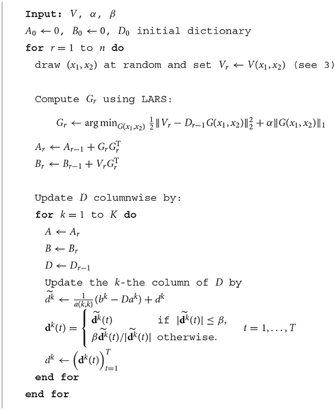
Algorithm 1. Double sparse OF decomposition.

4. Motion magnification

The detection of microexpressions and facial micro movements plays an increasingly important role for various applications from computer vision. Microexpressions and micromovements are often unobservable by the untrained and naked eye. This difficult task can be necessary in the context of the annotation of video datasets (e.g., compare [42]). The visualization of microexpressions and other micro movements in the face via motion magnification can potentially mitigate the difficulty of manual microexpression detection to enable manual annotation and microexpression analysis without professional or specific training. Furthermore, unsupervised selection and magnification of different motion components can help with exploratory investigation of facial micro movements for the development of new methods for remote assessment.

Having decomposed the OF field into meaningful spatial and temporal components, we show in this section how these components can be used to enhance the OF in the regions of interest and how this can be visualized in a new video sequence using a sophisticated warping method. Image warping is used in the context of OF estimation, compression or image registration (usually backwards warping), or for applications from graphics such as texture mapping or novel view synthesis, among the rich literature, see e.g., Brox et al. [19] and Wolberg [36].

4.1. Forward warping

For a given displacement v between two consecutive image frames f₁ and f₂ (so that we can skip the time variable), there are two prevalent methods for warping, forward warping and backward warping:

(i) Backward warping f₁ to yield f_bw:

$\begin{array}{l}{f}_{\text{bw}}(x_1,x_2):=f_1(x_1-v_1(x_1,x_2),x_2-v_2(x_1,x_2)).\end{array}$

Usually backward warping is preferred as it directly computes the warped frame. However, we will see that for warping facial motions, backward warping is far inferior to forward warping.

(ii) Forward warping f₁ to yield f_fw:

$\begin{array}{l}{f}_{\text{fw}}(x_1+v_1(x_1,x_2),x_2+v_2(x_1,x_2)):=f_1(x_1,x_2).\end{array}$

The difference between both warping methods is illustrated in Figure 1. This figure shows the results of forward warping vs. backward warping on a displacement field which corresponds to an magnified blinking motion as well as a magnification of the raising of an eyebrow. In this case, the motion field is localized on the eyebrow and the eyelid. Therefore, when doing backward warping, the colors stay exactly the same everywhere, and the displacement field is zero. In this illustration, this yields a contraction of the eyebrow and a contraction of the eye itself. This problem does not occur when doing forward warping.

FIGURE 1

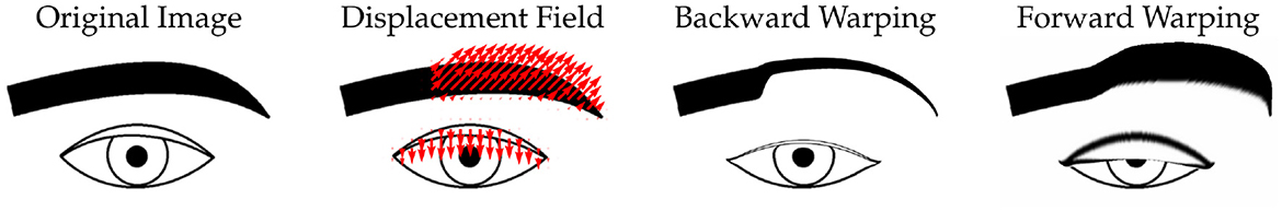
Figure 1. An illustration showing the results of forward vs. backward warping with an example displacement field.

However, in computer graphics, forward warping is significantly harder to do. This is because for the warped frame, we only have color information at the points (x₁ + v₁(x₁, x₂), x₂ + v₂(x₁, x₂)), which generally do not correspond to grid coordinates. To overcome this problem, we use the following scheme: first, we consider a triangulation of the frame f₁, which we aim to warp. The structure of this triangulation is shown in Figure 2 left. Each triangle connects three adjacent pixels and the vertices are equipped with the color values of the corresponding pixel. Then, the triangles are displaced according to the vector field (v₁, v₂), yielding a displaced triangulation depicted in Figure 2 right. Finally, each of the displaced triangles is rasterized. More precisely, we take all pixels whose midpoints are contained in the displaced triangle and assign them a value interpolating the triangle vertex color values using barycentric coordinates.

FIGURE 2

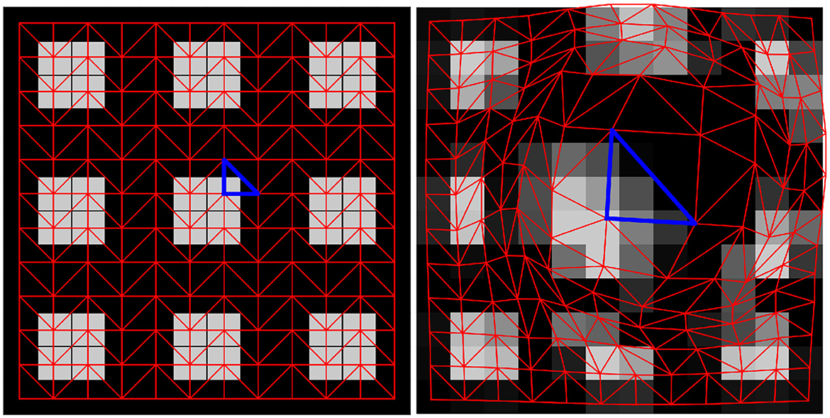
Figure 2. Illustration of the forward warping process. The image is first triangulated as shown on the left. The triangles are displaced and the warped image is then rasterized from these distorted triangles, see next figure.

Finally, it can be possible that multiple displaced triangles overlap. To resolve this ambiguity, the proposed algorithm allows for a depth map as the input which indicates which triangles should be drawn above others. While for this application, an elaborate depth map based on facial features could be devised, we opted to set the depth map such that stronger motions always “overlap” weaker motions.

To efficiently compute the triangulation, displacement, and subsequent rasterization of the input image, we employed a shader pipeline written using the OpenGL programming language. In short, this means that we make use of GPU native routines which are extremely efficient at handling such tasks and enable us to even employ this forward warping technique in real-time applications.

4.2. Motion magnification in selected regions

With all this at hand, we are now able to magnify selected movements in the input video. To this end, we still need to decide which components from the decomposition in Section 3 can be considered to be micro-movements. In our case, this is done by simply evaluating for each k ∈ {1, …, K}, if the values of d^k lie in a specified range. However, as the d^k are all normalized due to our optimization procedure, we need to adjust them to better resemble the velocity magnitudes from the OF. In short, we do the following selection:

1. Compute the maximum of each domain G^k for all k ∈ {1, …, K},

$\begin{array}{l}{m}_k:={\displaystyle \underset{x_1,x_2}{max}}{G}^k(x_1,x_2).\end{array}$

2. Compute the maximal normalized motion magnitude for each component

$c^k:=m^k\underset{{}_{t\in \{1,\dots ,T\}}}{\max }\left|\right|d^k(t)|{|}_2.$

3. For two pre-defined thresholds 0 < λ₁ < λ₂, consider the k-th component k ∈ {1, …, K} to belong to a micro-movement if ${\text{λ}}_1\le c^k\le {\text{λ}}_2.$

Let $\mathcal{I}\subset \left\{1,\dots ,K\right\}$ be the set of components deemed to correspond to micro-movements by the above selection. Then, we magnify their motion as follows. For each, t ∈ {1, …, T − 1}, we assume that v(t, ·) warps the frame f₁ into f₂. Therefore, magnification of the micro-movements by the magnification factor μ > 0, we aim to warp f₁ by the flow field

$\tilde{\text{v}}(t,·):=\text{ v}(t,·)+\mu {\displaystyle \sum _{k\in \mathcal{I}}{d}^k}(t)G^k(·).$

5. Experiments

We illustrate our proposed method on an example video from CASME II [42] and a video from the medical dataset for the remote detection of respiratory infections (see Figure 3). All our experiments were performed on consumer-grade computers. RAFT training has been performed on a multi-GPU machine with Intel Xeon Gold processors and two Nvidia Tesla V100 GPUs.

FIGURE 3

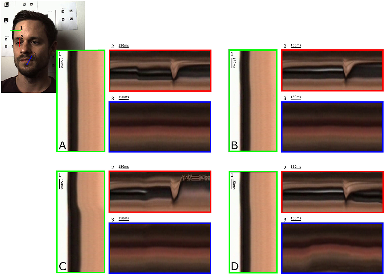
Figure 3. Experiments on the medical dataset with different parameters. The choice of parameters can be used to visualize different motion components when analyzing the video. [(A),2]: magnification of a subtle saccade before the blinking event with (η, λ, μ) = (3, 0.2, 10); [(B),2]: magnification of a larger saccade after blinking with (η, λ, μ) = (3, 0.4, 4); [(C),1]: magnification the subtle head motion with (η, λ, μ) = (4, 0.5, 8); [(D),3]: magnification of a micromovement of the mouth with (η, λ, μ) = (8, 0.3, 10). All results are with K = 9 and λ₁ = 0.1.

5.1. Datasets and data acquisition

CASME II and SMIC are datasets of spontaneous microexpressions which include 35 (CASME II) and 16 (SMIC) participants, respectively. Videos are recorded at 200 fps (CASME II) and 100 fps (SMIC). Each video is labeled with either observable or expected microexpressions, the latter based on self-reports of the participants.

Additionally, we use a video from a dataset for the remote assessment of respiratory diseases (VI-SCREEN). For this dataset, participants were recruited at multiple recording sites, including Saarland Univerisity Clinic (UKS) Children's Hospital and at the UKS central emergency admission, Germany. Recruitment happened from February 2022 and is ongoing (July 2023). Up until April 2023, this study includes 106 participants [median age 26 years, interquartile range (IQR) 24 years]. Informed consent was obtained, and the study was approved by the Ethics committee of the Ärztekammer des Saarlandes (02/22). Viral and bacterial, respiratory pathogens were tested using multiplex polymerase chain reaction (Multiplex PCR) assays. The camera array consisted of stereo RGB, near infrared (NIR) and thermal cameras as well as microphones [compare [50]]. A duration of 5–10 min was recorded, where participants answered questions in front of the camera. Core temperature was recorded with infrared ear thermometers. The videos in this dataset can contain microexpressions as well as other types of micro movements which are potentially related to symptoms of respiratory diseases. As benchmark sequence, we selected a video which contains a large movement (eye blinking) as well as a small movement around the mouth.

5.1.1. Motion estimation

We compare our method against RAFT-Sintel and RAFT-KITTI as well as against FlowFormer² after the same training schedules [51]. RAFT-Sintel performed better than RAFT-KITTI which is why we choose RAFT-Sintel as the baseline model for refinement. Due to the lack of publicly available datasets of facial microexpressions with ground truth OF annotation, we compared the methods by estimating a motion compensation error on a CASME II sequence from participant number 14.³ We used the mean squared error (MSE) of the gray values as well as on the Laplacian, see Figure 4.

FIGURE 4

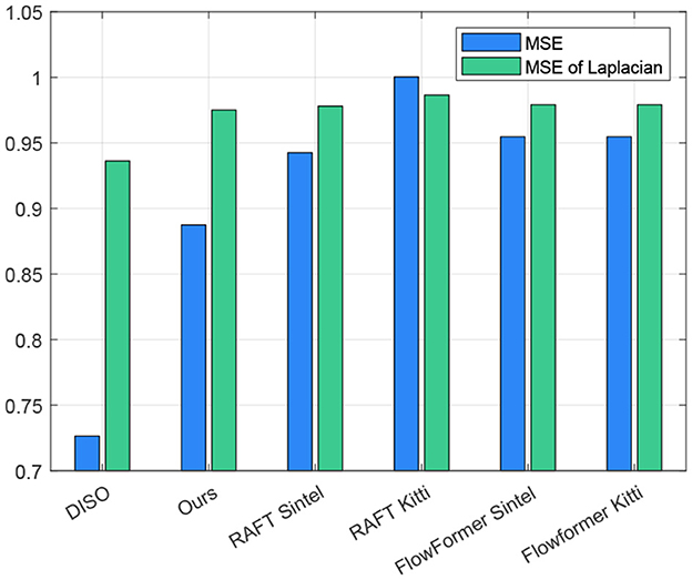
Figure 4. MSE for a sequence on a microexpression sequence after motion compensation. The values are normalized with respect to the MSE of the raw recording. While DISO performs better than the refined RAFT, our RAFT refinement on the ME dataset improved the performance over other state-of-the-art models trained on Sintel and KITTI-2015 in our examples.

While the performance of DISO was better on the test sequence than all other methods, our RAFT refinement with the ME dataset could generally improve performance on facial microexpression videos.

5.1.2. Motion magnification

For the motion magnification experiments, we used a video of participant number 14 from CASME II as well as a recording from the VI-SCREEN dataset. Participant number 14 has been excluded from the OF training dataset. The videos contain microexpressions and micromovements. We perform the analysis outlined in Section 3 using a sparsity regularization parameters α = 0.1, β = 4 and K = 9 components. A motion component k ∈ {1, …, 9} is selected to be a microexpression if ${\text{λ}}_1=0.1\le c^k\le {\text{λ}}_2=0.3$ holds true. We magnify these selected microexpressions using the magnification factor μ = 4.

Figure 5 shows an example application of our method with the sparse decomposition model (5) with ||·||_2,1 constraint. Our experiments show that our method is able to successfully decompose the OF field into reasonable components. Using this decomposition, we are able to perform facial motion magnification selectively in an unsupervised manner. For the case shown in Figure 5 the threshold corresponds only to the components connected to the micromovements around the mouth. The blinking motion is unchanged. Changing the thresholds also lets us select different motions. In Figure 6, we illustrate the results of our algorithm when choosing instead the thresholds λ₁ = 0.3 and λ₂ = ∞. In this case, only the blinking motion is magnified.

FIGURE 5

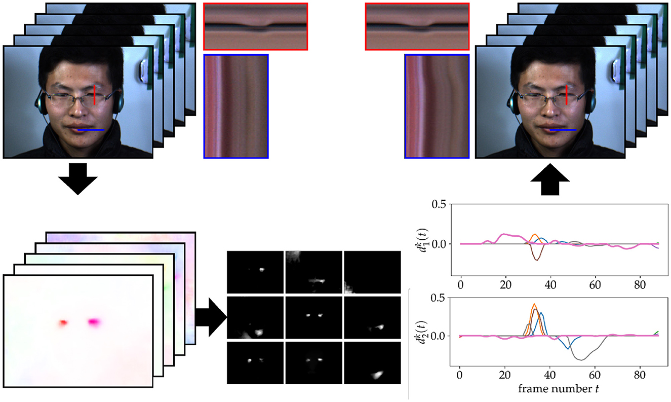
Figure 5. Illustration of our motion magnification procedure with the ||·||_2,1 -constraint. The algorithm starts with a sequence of 80 video frames of size 640 × 480 illustrated in the top left. The OF field computed for each time step is illustrated in the lower left. Then, we used our method to decompose this OF field into G¹, …, G⁹ shown in the bottom middle as well as the $(d_1^1,d_2^1),\dots ,(d_1^9,d_2^9)$ in the bottom right. In this example, two components, shown by thicker lines in the plot, were selected by thresholding to be micromovements. The frames are warped accordingly to yield the video sequence in the top right. The pixels from the red and blue lines are plotted over time in the corresponding red and blue boxes. This shows that the motion around the mouth is magnified while leaving the blinking motion unchanged.

FIGURE 6

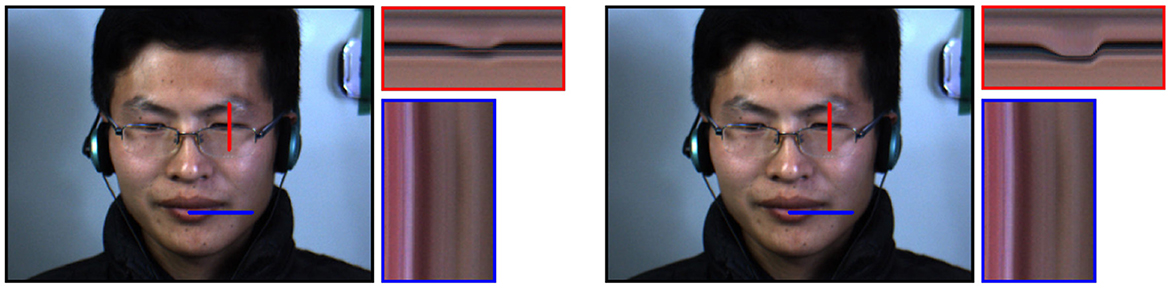
Figure 6. Illustration of the same video without (left) and with (right) motion magnification. The chosen thresholds (λ₁ = 0.3, λ₂ = ∞) only magnify the largest motions. This results in magnification of the blinking motion while leaving other facial movements unchanged.

For comparison, Figure 7 depicts the outcome of a similar experiment using just the ||·||₂ -constraint, see Remark 2. For this comparison, we use the same parameters α = 0.1, K = 9, and μ = 4. Introduction of the sparsity-promoting constraint leads to a clearer separation of motion components in the image as well as between temporally disconnected motions. We can observe this in the visualization of the components in Figure 8, where the ||·||_2,1 -constraint produces smaller components with clearer edges. Figure 9 shows how each component from the ||·||_2,1-constraint has only limited, temporal extend, while with the ||·||₂ -constraint, a few components capture a wide range of motion events over the complete video.

FIGURE 7

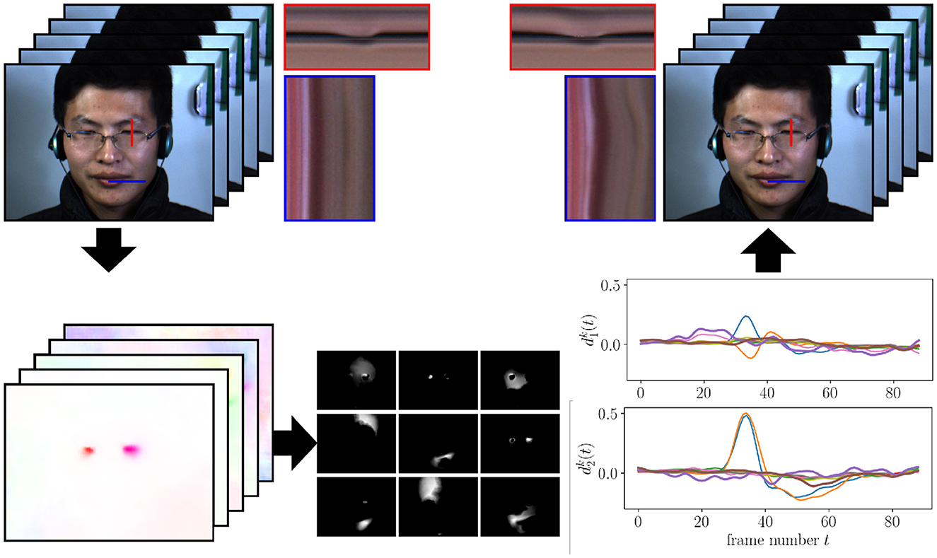
Figure 7. Illustration of our motion magnification procedure as in Figure 5, but with the  ·₂-constraint.

FIGURE 8

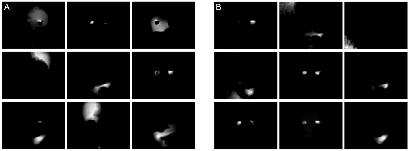
Figure 8. Illustration of the motion components G¹, …, G⁹ with the ∥·∥₂-constraint (A) and with the ∥·∥_2,1-constraint (B). The components in (B) show spatially smaller components with clearer edges.

FIGURE 9

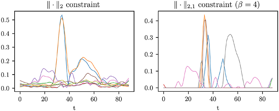
Figure 9. On the left-hand side, $\parallel d^k(t){\parallel }_2$ is shown over time for all nine components, where we optimized problem (6). On the right-hand side, we see the curves of $\left|\right|d^k(t)|{|}_{2,1}$ after optimizing problem (5). It can be observed that the later one promotes the separation of the flow field in temporally distinct motions, while in the first one a few components capture a wide range of motion events.

6. Conclusion

We provided a non-supervised method for magnifying micro-motions in facial videos based on the Lagrangian approach with OF forward warping magnification. The actual regions for OF magnification were found by minimizing a double sparse decomposition model for OF and a thresholding procedure to detect the relevant regions. Our thresholding method for differentiating microexpressions from other movements is open to further improvement. For example, the temporal extent of each motion could be taken into consideration. However, in the case of the CASME II dataset, where eye movements are the only notable facial motions beside microexpressions, a simple thresholding was already sufficient. Furthermore, significant head-movements might disrupt the presented decomposition into time-independent regions of motion in the face. In these cases, a facial alignment pre-processing step might be necessary. This could be realized similar to related studies [2, 11, 52] or by attenuating large and global motion with our method which might become more important with out-of-lab data with difficult motion. Moreover, our method has multiple parameters that need to be manually chosen. As a next step, statistics from real-world microexpression datasets could be included to learn suitable parameters for different motion types. The presented methods have the potential to facilitate the annotation of datasets with such face recordings for microexpression detection. Subtle expression changes, where the detection would otherwise require expert training, could be magnified for untrained individuals, who could then annotate such data. Our preliminary results with a real world, medical recording demonstrated how different parameters would allow for the visualization of different motion components in videos.

To the best to our knowledge, there exist no facial microexpression or micromovement datasets with ground truth OF. OF methods have been analyzed with respect to their predictive power of microexpressions [53] which does not allow conclusions on the overall quality of the OF predictions. Regarding the refinement of RAFT, future evaluations have to show the performance gain compared to OF methods tailored to faces with different training or transfer learning strategies such as Alkaddour et al. [54] for which the models are currently not publicly available. Given the small movements in the SMIC and CASME II recordings as well as constant backgrounds, further data augmentations that introduce large displacements and different background textures could further improve the method.

Data availability statement

The datasets presented in this article are not readily available because of restrictions from the General Data Protection Regulation with respect to personal data such as videos of faces. Requests to access the datasets should be directed to https://www.snnu.uni-saarland.de/.

Ethics statement

The studies involving humans were approved by Ethics Committee of the Ärztekammer des Saarlandes (02/22). The studies were conducted in accordance with the local legislation and institutional requirements. Written informed consent for participation was not required from the participants or the participants' legal guardians/next of kin in accordance with the national legislation and institutional requirements. Written informed consent was obtained from the individual(s) for the publication of any potentially identifiable images or data included in this article.

Author contributions

All authors listed have made a substantial, direct, and intellectual contribution to the work and approved it for publication.

Funding

This study has partially been funded by the Federal Ministry of Education and Research (BMBF, grant numbers 13N15753 and 13N15754).

Conflict of interest

The authors declare that the research was conducted in the absence of any commercial or financial relationships that could be construed as a potential conflict of interest.

Publisher's note

All claims expressed in this article are solely those of the authors and do not necessarily represent those of their affiliated organizations, or those of the publisher, the editors and the reviewers. Any product that may be evaluated in this article, or claim that may be made by its manufacturer, is not guaranteed or endorsed by the publisher.

Footnotes

1. ^https://sintel.is.tue.mpg.de/results

2. ^FlowFormer is among the top ten best performing methods on the Sintel benchmark [22] as of July 2023.

3. ^The benchmark video is EP04_04f from participant number 14.

References

1. Wu HY, Rubinstein M, Shih E, Guttag J, Durand F, Freeman W. Eulerian video magnification for revealing subtle changes in the world. ACM Trans Graph. (2012) 31:1–8. doi: 10.1145/2185520.2185561

PubMed Abstract | CrossRef Full Text | Google Scholar

2. Elgharib M, Hefeeda M, Durand F, Freeman WT. Video magnification in presence of large motions. In: Proceedings of the IEEE Computer Social Conference Computer Vision Pattern Recognition. (2015). p. 4119–4127. doi: 10.1109/CVPR.2015.7299039

CrossRef Full Text | Google Scholar

3. Wadhwa N, Rubinstein M, Durand F, Freeman WT. Phase-based video motion processing. ACM Trans Graph. (2013) 32:80. doi: 10.1145/2461912.2461966

CrossRef Full Text | Google Scholar

4. Zhang Y, Pintea SL, Van Gemert JC. Video acceleration magnification. In: Proceedings of the IEEE Computer Social Conference Computer Vision Pattern Recognition. (2017). p. 529–537. doi: 10.1109/CVPR.2017.61

CrossRef Full Text | Google Scholar

5. Sarrafi A, Mao Z, Niezrecki C, Poozesh P. Vibration-based damage detection in wind turbine blades using Phase-based Motion Estimation and motion magnification. J Sound Vib. (2018) 421:300–18. doi: 10.1016/j.jsv.2018.01.050

CrossRef Full Text | Google Scholar

6. Eitner M, Musta M, Vanstone L, Sirohi J, Clemens N. Modal parameter estimation of a compliant panel using phase-based motion magnification and stereoscopic digital image correlation. Exper Tech. (2021) 45:287–96. doi: 10.1007/s40799-020-00393-6

CrossRef Full Text | Google Scholar

7. Fei J, Xia Z, Yu P, Xiao F. Exposing AI-generated videos with motion magnification. Multimed Tools Appl. (2021) 80:30789–802. doi: 10.1007/s11042-020-09147-3

CrossRef Full Text | Google Scholar

8. Alinovi D, Ferrari G, Pisani F, Raheli R. Respiratory rate monitoring by video processing using local motion magnification. In: Proceedings of the European Signal Processing Conference EUSIPCO. IEEE (2018). p. 1780–1784. doi: 10.23919/EUSIPCO.2018.8553066

CrossRef Full Text | Google Scholar

9. Bai J, Agarwala A, Agrawala M, Ramamoorthi R. Selectively de-animating video. ACM Trans Graph. (2012) 31:66–1. doi: 10.1145/2185520.2185562

CrossRef Full Text | Google Scholar

10. Liu C, Torralba A, Freeman WT, Durand F, Adelson EH. Motion magnification. ACM Trans Graph. (2005) 24:519–526. doi: 10.1145/1073204.1073223

CrossRef Full Text | Google Scholar

11. Flotho P, Bhamborae MJ, Haab L, Strauss DJ. Lagrangian motion magnification revisited: Continuous, magnitude driven motion scaling for psychophysiological experiments. In: Annual International Conference IEEE Engineering Medical Biology Social. IEEE (2018). p. 3586–3589. doi: 10.1109/EMBC.2018.8512892

PubMed Abstract | CrossRef Full Text | Google Scholar

12. Flotho P, Nomura S, Kuhn B, Strauss DJ. Software for non-parametric image registration of 2-photon imaging data. J Biophotonics. (2022) 15:e202100330 doi: 10.1002/jbio.202100330

PubMed Abstract | CrossRef Full Text | Google Scholar

13. Hartmann C, Weiss HA, Lechner P, Volk W, Neumayer S, Fitschen JH, et al. Measurement of strain, strain rate and crack evolution in shear cutting. J Mater Process Technol. (2021) 288:116872. doi: 10.1016/j.jmatprotec.2020.116872

CrossRef Full Text | Google Scholar

14. Strauss DJ, Corona-Strauss FI, Schroeer A, Flotho P, Hannemann R, Hackley SA. Vestigial auriculomotor activity indicates the direction of auditory attention in humans. Elife. (2020) 9:e54536. doi: 10.7554/eLife.54536

PubMed Abstract | CrossRef Full Text | Google Scholar

15. Chen Z, Jin H, Lin Z, Cohen S, Wu Y. Large displacement optical flow from nearest neighbor fields. In: Proceedings of the IEEE Computer Social Conference Computer Vision Pattern Recognition. (2013). p. 2443–2450. doi: 10.1109/CVPR.2013.316

PubMed Abstract | CrossRef Full Text | Google Scholar

16. Baker S, Scharstein D, Lewis JP, Roth S, Black MJ, Szeliski R, et al. database and evaluation methodology for optical flow. Int J Comput Vis. (2011) 92:1–31. doi: 10.1007/s11263-010-0390-2

CrossRef Full Text | Google Scholar

17. Sun D, Roth S, Black MJ. Secrets of optical flow estimation and their principles. In: 2010 IEEE Computer Society Conference on Computer Vision and Pattern Recognition. IEEE (2010). p. 2432–2439. doi: 10.1109/CVPR.2010.5539939

CrossRef Full Text | Google Scholar

18. Kroeger T, Timofte R, Dai D, Van Gool L. Fast optical flow using dense inverse search. In: Computer Vision ECCV. Springer (2016). p. 471–488. doi: 10.1007/978-3-319-46493-0_29

CrossRef Full Text | Google Scholar

19. Brox T, Bruhn A, Papenberg N, Weickert J. High accuracy optical flow estimation based on a theory for warping. In: Computer Vision ECCV. Springer (2004). p. 25–36. doi: 10.1007/978-3-540-24673-2_3

CrossRef Full Text | Google Scholar

20. Mayer N, Ilg E, Hausser P, Fischer P, Cremers D, Dosovitskiy A, et al. A large dataset to train convolutional networks for disparity, optical flow, and scene flow estimation. In: Proceedings of the IEEE Computer Social Conference Computer Vision Pattern Recognition. (2016). p. 4040–4048. doi: 10.1109/CVPR.2016.438

CrossRef Full Text | Google Scholar

21. Teed Z, Deng J. Raft: Recurrent all-pairs field transforms for optical flow. In: Computer Vision ECCV. Springer (2020). p. 402–419. doi: 10.1007/978-3-030-58536-5_24

PubMed Abstract | CrossRef Full Text | Google Scholar

22. Butler DJ, Wulff J, Stanley GB, Black MJ. A naturalistic open source movie for optical flow evaluation. In: Fitzgibbon A., , editor European Conference on Computer Vision (ECCV) Part IV, LNCS 7577. Springer-Verlag (2012). p. 611–625. doi: 10.1007/978-3-642-33783-3_44

CrossRef Full Text | Google Scholar

23. Sun D, Herrmann C, Reda F, Rubinstein M, Fleet DJ, Freeman WT. Disentangling architecture and training for optical flow. In: European Conference on Computer Vision (ECCV). Springer (2022). p. 165–182. doi: 10.1007/978-3-031-20047-2_10

CrossRef Full Text | Google Scholar

24. Yan WJ, Wu Q, Liang J, Chen YH, Fu X. How fast are the leaked facial expressions: The duration of micro-expressions. J Nonverbal Behav. (2013) 37:217–30. doi: 10.1007/s10919-013-0159-8

CrossRef Full Text | Google Scholar

25. Huang X, Wang SJ, Liu X, Zhao G, Feng X, Pietikäinen M. Discriminative spatiotemporal local binary pattern with revisited integral projection for spontaneous facial micro-expression recognition. IEEE Trans Affect Comput. (2017) 10:32–47. doi: 10.1109/TAFFC.2017.2713359

CrossRef Full Text | Google Scholar

26. Xu F, Zhang J, Wang JZ. Microexpression identification and categorization using a facial dynamics map. IEEE Trans Affect Comput. (2017) 8:254–67. doi: 10.1109/TAFFC.2016.2518162

CrossRef Full Text | Google Scholar

27. N L, C A, A J, W PRC, J S. Micro-expression motion magnification: Global Lagrangian vs. local Eulerian approaches. In: IEEE International Conference Automation Face Gesture Recognition Workshops. IEEE (2018). p. 650–656.

Google Scholar

28. Zhang L, Arandjelović O. Review of automatic microexpression recognition in the past decade. Mach Learn Knowl Extr. (2021) 3:414–34. doi: 10.3390/make3020021

CrossRef Full Text | Google Scholar

29. Shan L, Yu M. Video-based heart rate measurement using head motion tracking and ICA. In: 2013 6th International Congress on Image and Signal Processing (CISP). IEEE (2013). p. 160–164. doi: 10.1109/CISP.2013.6743978

CrossRef Full Text | Google Scholar

30. Mroueh Y, Marcheret E, Goel V. Deep multimodal learning for audio-visual speech recognition. In: Proceedings of the IEEE International Conference Acoustic Speech Signal Process. IEEE (2015). p. 2130–2134. doi: 10.1109/ICASSP.2015.7178347

PubMed Abstract | CrossRef Full Text | Google Scholar

31. Mairal J, Bach F, Ponce J, Sapiro G. Online dictionary learning for sparse coding. In: Annual International Conference on Machine Learning ICML '09. New York, NY, USA: Association for Computing Machinery (2009). p. 689–696. doi: 10.1145/1553374.1553463

PubMed Abstract | CrossRef Full Text | Google Scholar

32. Beinert R, Steidl G. Robust PCA via regularized REAPER with a matrix-free proximal algorithm. J Mathem Imag Vis. (2021) 63:626–649. doi: 10.1007/s10851-021-01019-1

PubMed Abstract | CrossRef Full Text | Google Scholar

33. Cabral R, la Torre FD, Costeira J, Bernardino A. Unifying nuclear norm and bilinear factorization approaches for low-rank matrix decomposition. In: Proceedings of the 2013 IEEE International Conference on Computer Vision. (2013). doi: 10.1109/ICCV.2013.309

CrossRef Full Text | Google Scholar

34. Candés E, Li X, Ma Y, Wright J. Robust principal component analysis? J ACM. (2011) 58:1–37. doi: 10.1145/1970392.1970395

CrossRef Full Text | Google Scholar

35. Holler M, Kunisch K. On infimal convolution of TV-type functionals and applications to video and image reconstruction. SIAM J Imag Sci. (2014) 7:2258–300. doi: 10.1137/130948793

CrossRef Full Text | Google Scholar

36. Wolberg G. Digital Image Warping. New York: Wiley-IEEE Computer Society Press (1990).

Google Scholar

37. Horn BKP, Schunck BG. Determining optical flow. Art Intelligence. (1981) 17:185–203. doi: 10.1016/0004-3702(81)90024-2

CrossRef Full Text | Google Scholar

38. Becker F, Petra S, Schnörr C. Optical Flow. In: Handbook of Mathematical Methods in Imaging. New York: Springer (2015). p. 1945–2004. doi: 10.1007/978-1-4939-0790-8_38

CrossRef Full Text | Google Scholar

39. Dosovitskiy A, Fischer P, Ilg E, Häusser P, Hazırbaş C, Golkov V, et al. FlowNet: learning optical flow with convolutional networks. In: IEEE International Conference on Computer Vision (ICCV). (2015). doi: 10.1109/ICCV.2015.316

CrossRef Full Text | Google Scholar

40. Menze M, Geiger A. Object scene flow for autonomous vehicles. In: Proceedings of the IEEE Conference on Computer Vision and Pattern Recognition. (2015). p. 3061–3070. doi: 10.1109/CVPR.2015.7298925

CrossRef Full Text | Google Scholar

41. Kondermann D, Nair R, Honauer K, Krispin K, Andrulis J, Brock A, et al. The HCI benchmark suite: Stereo and flow ground truth with uncertainties for urban autonomous driving. In: Proceedings of the IEEE Conference on Computer Vision and Pattern Recognition Workshops. (2016). p. 19–28. doi: 10.1109/CVPRW.2016.10

CrossRef Full Text | Google Scholar

42. Yan WJ Li X, Wang SJ, Zhao G, Liu YJ, Chen YH, et al. CASME II: An improved spontaneous micro-expression database and the baseline evaluation. PLoS ONE. (2014) 9:e86041. doi: 10.1371/journal.pone.0086041

PubMed Abstract | CrossRef Full Text | Google Scholar

43. Li X, Pfister T, Huang X, Zhao G, Pietikäinen M. A spontaneous micro-expression database: Inducement, collection and baseline. In: IEEE International Conference Automation Face Gesture Recognition Workshops. IEEE (2013). p. 1–6. doi: 10.1109/FG.2013.6553717

CrossRef Full Text | Google Scholar

44. Bradski G. The OpenCV library. Dr Dobb's J Softw Tools. (2000) 120:122–125.

Google Scholar

45. Beck A. First-Order Methods in Optimization. Philadelphia: Society for Industrial and Applied Mathematics (SIAM), Mathematical Optimization Society. (2017). doi: 10.1137/1.9781611974997

CrossRef Full Text | Google Scholar

46. Burger M, Sawatzky A, Steidl G. First Order algorithms in variational image processing. In:Glowinski R, Osher SJ, Yin W, , editors. Splitting Methods in Communication, Imaging, Science, and Engineering. Cham: Springer (2016). p. 345–407. doi: 10.1007/978-3-319-41589-5_10

CrossRef Full Text | Google Scholar

47. Osborne MR, Presnell B, Turlach BA, A. new approach to variable selection in least squares problems. IMA J Numer Anal. (2000) 20:389–403. doi: 10.1093/imanum/20.3.389

CrossRef Full Text | Google Scholar

48. Efron B, Hastie T, Johnstone I, Tibshirani R. Least angle regression. Ann Stat. (2004) 32:407–99. doi: 10.1214/009053604000000067

CrossRef Full Text | Google Scholar

49. Bertsekas DP. Nonlinear Programming. Nashua NH: Athena Scientific Belmont. (1999).

Google Scholar

50. Flotho P, Bhamborae MJ, Grün T, Trenado C, Thinnes D, Limbach D, et al. Multimodal data acquisition at SARS-CoV-2 drive through screening centers: Setup description and experiences in Saarland, Germany. J Biophotonics. (2021) 14:e202000512. doi: 10.1002/jbio.202000512

PubMed Abstract | CrossRef Full Text | Google Scholar

51. Huang Z, Shi X, Zhang C, Wang Q, Cheung KC, Qin H, et al. FlowFormer: a transformer architecture for optical flow. arXiv preprint. arXiv:220316194. (2022). doi: 10.1007/978-3-031-19790-1_40

CrossRef Full Text | Google Scholar

52. Flotho P, HeißC, Steidl G, Strauss DJ. Lagrangian motion magnification with landmark-prior and sparse PCA for facial microexpressions and micromovements. In: Annual International Conference IEEE Engineering Medical Biology Social. IEEE (2022). p. 2215–2218. doi: 10.1109/EMBC48229.2022.9871549

PubMed Abstract | CrossRef Full Text | Google Scholar

53. Allaert B, Ward IR, Bilasco M, Djeraba C, Bennamoun M. A comparative study on optical flow for facial expression analysis. Neurocomputing. (2022). doi: 10.1016/j.neucom.2022.05.077

CrossRef Full Text | Google Scholar

54. Alkaddour M, Tariq U, Dhall A. Self-supervised approach for facial movement based optical flow. arXiv:2105.01256. (2021). doi: 10.1109/TAFFC.2022.3197622

CrossRef Full Text | Google Scholar