A lifted Bregman formulation for the inversion of deep neural networks

1. Introduction

Neural networks are computing systems that have revolutionized a wide range of research domains over the past decade and outperformed many traditional machine learning approaches [cf. [1, 2]]. This performance often comes at the cost of interpretability (or rather a lack thereof) of the outputs that a neural network produces for given inputs. As a consequence, a lot of research has focused on understanding representations of neural networks and on developing strategies to interpret these representations, predominantly with saliency maps [3–6]. An alternative approach focuses on understanding deep image representations by inverting them [7]. The authors propose a total-variation-based variational optimization method that aims to infer the network input from the network output with regularized inversion.

While the concept of inverting neural networks is certainly not new [cf. [8–11]], there has been increasing interest in recent years largely due to developments in nonlinear dimensionality reduction and generative modeling that include (but are not limited to) (variational) Autoencoders [12], Normalizing Flows [13, 14], Cycle-Consistent Generative Adversarial Networks [15], and Probabilistic Diffusion Models [16, 17].

While several approaches for the inversion of neural networks have been proposed especially in the context of generative modeling [see for example [18, 19] in the context of normalizing flows, [20] in the context of generative adversarial networks, and [21] in the context of probabilistic diffusion models] an important aspect, which is often overlooked, is that invertible operations alone are not automatically stable with respect to small variations in the data. For example, computing the solution of the heat equation after a fixed termination time is stable with respect to variations in the initial condition, but estimating the initial condition from the terminal condition of the heat equation is not stable with respect to perturbations in the terminal condition. This issue cannot be resolved without approximation of the inverse with a family of continuous operators, also known as regularization. The research field of Inverse and Ill-posed Problems and its branch Regularization Theory focus strongly on the stable approximation of ill-posed and ill-conditioned inverses via regularizations [22] and so-called variational regularizations [23, 24] that are a special class of (nonlinear) regularizations. The optimization model proposed in [7] can be considered as a variational regularization method with total variation regularization; however, the work in Mahendran and Vedaldi [7] is purely empirical, and to the best of our knowledge no works exist that rigorously prove that the proposed approach is a variational regularization.

In this work, we propose a novel regularization framework based on lifting with tailored Bregman distances and prove that the proposed framework is a convergent variational regularization for the inverse problem of estimating the inputs from single-layer perceptrons or the inverse problem of estimating hidden variables in a multi-layer perceptron sequentially. While there has been substantial work in previous years that focuses on utilizing neural networks as nonlinear operators in variational regularization methods [25–29], this is the first work that provides theoretical guarantees for the stable, model-based inversion of neural networks to the best of our knowledge.

Our contributions are three-fold. (1) We propose a novel framework for the regularized inversion of multi-layer perceptrons, respectively feed-forward neural networks, that is based on the lifted Bregman framework recently proposed by the authors in [30]. (2) We show that for the single-layer perceptron case, the proposed variational regularization approach is a provably convergent regularization under very mild assumptions. To our knowledge, this is the first time that an inversion method has been proposed that does not just allow to perform inversion empirically, but for which we can prove that the proposed method is a convergent regularization method without overly restrictive assumptions such as differentiability of the activation function and the presence of a tangential cone condition. (3) We propose a proximal first-order optimization strategy to solve the proposed variational regularization method and present several numerical examples that support the effectiveness of the proposed model-based regularization approach.

The paper is structured as follows. In Section 2, we introduce the lifted Bregman formulation for the model-based inversion of feed-forward neural networks. In Section 3, we prove that for the single-layer perceptron case the proposed model is a convergent variational regularization method and provide general error estimates as well as error estimates for a concrete example of a perceptron with ReLU activation function. In Section 4, we discuss how to implement the proposed variational regularization computationally for both the single-layer and multi-layer perceptron setting with a generalization of the primal-dual hybrid gradient method and coordinate descent. Subsequently, we present numerical results that demonstrate empirically that the proposed approach is a model-based regularization in Section 5, before we conclude this work with a brief section on conclusions and outlook in Section 6.

2. Model-based inversion of feed-forward networks

Suppose we are given an L-layer feed-forward neural network $\mathcal{N}:{ℝ}^n\times \mathcal{P}\to {ℝ}^m$ of the form

$\begin{array}{ll}\mathcal{N}(x,\Theta )={\sigma }_L(f({\sigma }_{L-1}(f(\dots {\sigma }_1(f(x,{\Theta }_1))\dots )),{\Theta }_L)),& (1)\end{array}$

for input data x ∈ ℝⁿ and pre-trained parameters $\Theta \in \mathcal{P}$. Here, ${\left\{{\sigma }_l\right\}}_{l=1}^L$ denotes the collection of nonlinear activation functions and f denotes a generic function parameterized by parameters ${\left\{{\Theta }_l\right\}}_{l=1}^L$. For ease of notation, we use Θ to refer to all parameters ${\left\{{\Theta }_l\right\}}_{l=1}^L$. For a given network output y ∈ ℝ^m, our goal is to solve the inverse problem

$\begin{array}{ll}\mathcal{N}(x,\Theta )=y& (2)\end{array}$

for the unknown input x ∈ ℝⁿ. The problem (2) is usually ill-posed in the sense that a solution may not exist (especially if n ≪ m) or is not unique (especially if m ≪ n, or if information is lost through application of nonlinear activation functions). Moreover, even for a network with identity activation functions σ_l and affine linear transformation f, solving (2) is often ill-conditioned in the sense that errors in y get heavily amplified when solving for x. We therefore, propose to approximate the inverse of this nonlinear, potentially ill-posed inverse problem via the minimization of a lifted Bregman formulation of the form

$\begin{array}{ll}\left(\begin{array}{c}{x}^{\alpha }\\ x_1^{\alpha }\\ ⋮\\ x_{L-1}^{\alpha }\end{array}\right)\in {\displaystyle \underset{x,x_1,\dots ,x_{L-1}}{arg min}}\left\{{\displaystyle \sum _{l=1}^L}{B}_{{\text{Ψ}}_l}(x_l,f(x_{l-1},{\Theta }_l))+\alpha R(x)\right\},& (3)\end{array}$

where we assume x₀ = x and $x_L=y^{\delta }$ for simplicity of notation. The data y^δ is a perturbed version of y, for which we assume $B_{{\text{Ψ}}_L}\left[y^{\delta },f(x_{L-1}^{†},{\Theta }_L)\right]\le {\delta }^2$, for some constant δ ≥ 0 and $y={\sigma }_L\left[f(x_{L-1}^{†},{\Theta }_L)\right]$. Please note that this approach is referred to as “lifted” because the solution space is lifted to a higher dimensional space that also includes auxiliary variables $x_l^{\alpha }$ for all intermediate layers. The functions B_Ψl for l = 1, …, L are defined as

$\begin{array}{ll}{B}_{{\text{Ψ}}_l}(x,z)=\frac{1}{2}||x{||}^2+{\text{Ψ}}_l(x)+{\left(\frac{1}{2}||·{||}^2+{\text{Ψ}}_l\right)}^{*}(z)-\langle x,z\rangle ,& (4)\end{array}$

for a proper, convex, and lower semi-continuous function ${\text{Ψ}}_l:{ℝ}^{n_l}\to ℝ\cup \left\{\infty \right\}$. The notation ${\left(\frac{1}{2}||·{||}^2+{\text{Ψ}}_l\right)}^{*}$ refers to the convex or Fenchel conjugate of $\frac{1}{2}||·{||}^2+{\text{Ψ}}_l$, i.e., ${\left(\frac{1}{2}||·{||}^2+{\text{Ψ}}_l\right)}^{*}\left(z\right)={sup}_y\langle z,y\rangle -\frac{1}{2}||y{||}^2-{\text{Ψ}}_l\left(y\right)$. Last but not least, the function R:ℝⁿ → ℝ∪{∞} is a proper, convex, and lower semi-continuous function that enables us to incorporate a-priori information into the inversion process. The impact of this is controlled by the parameter α > 0.

Please note that the functions B_Ψl are directly connected to the chosen activation functions ${\left\{{\sigma }_l\right\}}_{l=1}^L$. Following [30], we observe

$\begin{array}{l}{B}_{{\text{Ψ}}_l}(x,z)\ge \frac{1}{2}||{\sigma }_l(z)-x{||}^2,\end{array}$

where ${\sigma }_l:{ℝ}^{n_l}\to {ℝ}^{n_l}$ is the proximal map with respect to Ψ_l, i.e.

$\begin{array}{l}{\sigma }_l(z)={\displaystyle \underset{y\in {ℝ}^{n_l}}{arg min}}\left\{\frac{1}{2}||y-z{||}^2+{\text{Ψ}}_l(y)\right\},\end{array}$

for all l ∈ {1, …, L}. This means that we will solely focus on feed-forward neural networks with nonlinear activation functions that are proximal maps.

The advantage of using functions B_Ψl over more conventional functions such as the squared Euclidean norm of the difference of the network output and the measured output, i.e., $\frac{1}{2}||\mathcal{N}(x,\Theta )-y{||}^2$, is that the functions B_Ψl are continuously differentiable with respect to their second argument [along with several other useful properties, cf. [30], Theorem 10]. If we define $F_x^l(z):=B_{{\text{Ψ}}_l}(x,z)$, we observe

$\begin{array}{ll}\nabla F_x^l(z)={\sigma }_l(z)-x.& (5)\end{array}$

Please note that the family of objective functions B_Ψl satisfies several other interesting properties; we refer the interested reader to [30], Theorem 10.

For the remainder of this work, we assume that the parameterized functions f are affine-linear in the first argument, with parameters Θ_l. A concrete example is the affine-linear transformation f(x, Θ_l) = W_lx + b_l, for a (weight) matrix $W_l\in {ℝ}^{n_l\times n_{l-1}}$, a (bias) vector $b_l\in {ℝ}^{n_l}$ and the collection of parameters Θ_l = (W_l, b_l).

In the next section, we show that (3) is a variational regularization method for L = 1 and prove a convergence rate with which the solution of (3) converges toward the true input of a perceptron when δ converges to zero.

3. Convergence analysis and error estimates

In this section, we show that the proposed model (3) is a convergent variational regularization for the specific choice L = 1 and the assumption f(x, Θ) = Wx + b for Θ = (W, b), which reduces (3) to a variational regularization model for the perceptron case studied in Wang and Benning [31]. In contrast to Wang and Benning [31] we are not interested in estimating the perceptron parameters W and b but assume that these are fixed, and that we study the regularization operator

$\begin{array}{l}{\mathcal{R}}_{\alpha }:\text{dom}(\Psi )\rightrightarrows {ℝ}^n,\\ {\mathcal{R}}_{\alpha }:y^{\delta }\rightrightarrows x_{\alpha }\in \underset{x\in {ℝ}^n}{\mathrm{arg min}}\left\{B_{\Psi }\left(y^{\delta },Wx+b\right)+\alpha R(x)\right\},& (6)\end{array}$

where dom(Ψ) is defined as dom(Ψ): = {y ∈ ℝ^m|Ψ(y) < ∞}. We first want to establish under which assumptions (6) is well-defined for all y^δ.

3.1. Well-definedness

For simplicity, we focus on the finite-dimensional setting with network inputs in ℝⁿ and outputs in dom(Ψ). However, the following analysis also extends to more general Banach space settings with additional assumptions on the operator W, see for instance [24], Section 5.1. Following [24], we assume that R is non-negative and the polar of a proper function, i.e., R = H^* for a proper function H:ℝⁿ → ℝ∪{∞}. Note that this automatically implies convexity of R. Moreover, we assume that Ψ is a proper, non-negative and convex function that is continuous on dom(Ψ), which implies that B_Ψ is proper, non-negative, convex in its second argument and continuous in its first argument for every y^δ ∈ dom(Ψ). Then, for every g ∈ dom(Ψ) there exists x with

$\begin{array}{l}{B}_{\text{Ψ}}(g,Wx+b)+\alpha R(x)<\infty .\end{array}$

Last but not least, we assume that R and Ψ are chosen such that for each g ∈ dom(Ψ) and α > 0 we have

$\begin{array}{l}||x||\le c(a,b,||g||),\text{if}{B}_{\text{Ψ}}(g,Wx+b)\le a\text{and}\alpha R(x)\le d,\end{array}$

for constants a, d, and a constant c that depends monotonically non-decreasing on all arguments. With these assumptions, we can then verify the following lemma.

Theorem 1. Let the assumptions outlined in the previous paragraph be satisfied.

1. Then, for every $y\in \{g\in \text{dom}(\Psi )|\mathrm{arg }{\min }_{x,\in {ℝ}^{\text{n}},\text{R}(x)<\infty }{B}_{\Psi }(g,Wx+b)\ne \varnothing \}$ the selection operator

$\begin{array}{l}\mathcal{S}(y)={\displaystyle \underset{x\in {ℝ}^n}{arg min}}\left\{R(x)|x\in {\displaystyle \underset{\tilde{x}\in {ℝ}^n}{arg min}}{B}_{\text{Ψ}}(y,W\tilde{x}+b)\right\}\end{array}$

is well-defined.

2. The regularization operator ${\mathcal{R}}_{\alpha }$ as defined in (3) is well-defined in the sense that for every y ∈ dom(Ψ) there exists $x_{\alpha }\in {ℝ}^n$ with $x_{\alpha }\in {\mathcal{R}}_{\alpha }(y)$. Moreover, the set ${\mathcal{R}}_{\alpha }(y)$ is a convex set.

3. For every sequence y_n→y ∈ dom(Ψ) there exists a subsequence $x_{n_k}\in {\mathcal{R}}_{\alpha }(y_{n_k})$ converging to an element $x^{*}\in {\mathcal{R}}_{\alpha }(y)$.

Proof. The results follow directly from [24], Lemma 5.5, Theorem 5.6, and Theorem 5.7. The latter statement originally only implies convergence in the weak-star topology; however, since we are in a finite-dimensional Hilbert space, this automatically implies strong convergence here.

3.2. Error estimates

Having established that (3) is a regularization operator, we now want to prove that it is also a convergent regularization operator in the sense of the estimate

$\begin{array}{ll}{D}_R(x^{†},x^{\alpha })\le C\delta ,& (7)\end{array}$

such that

$\begin{array}{l}\underset{\delta \to 0}{\lim }\sup \{D_R(x^{†},x^{\alpha })|x^{\alpha }\in {\mathcal{\text{R}}}_{\alpha }(y^{\delta }),y^{\delta }\in \text{dom}(\Psi ),\\ B_{{}_{\Psi }}(y^{\delta },W{x}^{†}+b)\le {\delta }^2\}=0.\end{array}$

Here, the term D_R denotes the (generalized) Bregman distance [or divergence, [cf. [32, 33]] with respect to R, i.e.,

$\begin{array}{l}{D}_R(x,\tilde{x})=R(x)-R(\tilde{x})-\langle \tilde{q},x-\tilde{x}\rangle ,\end{array}$

for two arguments $x,\tilde{x}\in \text{dom}(R)$ and a subgradient $\tilde{q}\in \partial R(\tilde{x})=\left\{q\in {ℝ}^n|R(x)\ge R(\tilde{x})+\langle q,x-\tilde{x}\rangle ,\forall x\in \mathrm{\text{dom}}(R)\right\}$. The vector x^α is a solution of (3) with data y^δ for which we assume $B_{\text{Ψ}}(y^{\delta },W{x}^{†}+b)\le {\delta }^2$, and C ≥ 0 is a constant. The vector x^† is an element of the selection operator as specified in Lemma 1. 1, i.e., $x^{†}\in \mathcal{S}(y)$ for y ∈ dom(Ψ). Note that $x^{†}\in \mathcal{S}(y)$ is equivalent to x^† being a R-minimizing vector amongst all vectors that satisfy 0 = W^*(σ(Wx^† + b) − y), where σ denotes the proximal map with respect to Ψ. This is due to the fact that $x^{†}\in {arg min}_{\tilde{x}\in {ℝ}^n}{B}_{\text{Ψ}}(y,W\tilde{x}+b)$ is equivalent to $0=\nabla B_{\text{Ψ}}(y,W{x}^{†}+b)=W^{*}(\sigma (W{x}^{†}+b)-y)$. Assuming that σ(Wx^† + b) − y does not lie in the nullspace of W^*, this further implies y = σ(Wx^† + b).

In order to be able to derive error estimates of the form (7), we restrict ourselves to solutions x^† that are in the range of ${\mathcal{R}}_{\alpha }$. This means that there exists y^† such that $x^{†}\in {\mathcal{R}}_{\alpha }(y^{†})$. Considering the optimality condition of (3) for y^†, this implies

$\begin{array}{l}{W}^{*}\left(\frac{y^{†}-\sigma (W{x}^{†}+b)}{\alpha }\right)\in \partial R(x^{†}),\end{array}$

which for v^†: = (y^† − σ(Wx^† + b))/α = (y^† − y)/α is equivalent to the existence of a source condition element v^† that satisfies the source condition [cf. [22, 24]].

$\begin{array}{ll}{W}^{*}{v}^{†}\in \partial R(x^{†}),& (\mathrm{SC})\end{array}$

In the following, we verify that the symmetric Bregman distance with respect to R between a solution of the regularization operator and the solution of the inverse problem is converging to zero if the error in the data is converging to zero. The symmetric Bregman distance or Jeffreys distance between two vectors x and $\tilde{x}$ simply is the sum of two Bregman distances with interchanged arguments, i.e.,

$\begin{array}{l}{D}_R^{\text{symm}}(x,\tilde{x}):=D_R(x,\tilde{x})+D_R(\tilde{x},x)=\langle x-\tilde{x},q-\tilde{q}\rangle ,\end{array}$

for q ∈ ∂R(x) and $\tilde{q}\in \partial R(\tilde{x})$; hence, an error estimate in the symmetric Bregman distance also implies an error estimate in the classical Bregman distance.

Before we begin our analysis, we recall the concept of the Jensen-Shannon divergence [34], which for general proper, convex and lower semi-continuous functions F:ℝⁿ → ℝ∪{∞} generalizes to so-called Burbea-Rao divergences [35–37] and are defined as follows.

Definition 1 (Burbea-Rao divergence). Suppose F:ℝⁿ → ℝ∪{∞} is a proper, convex and lower semi-continuous function. The corresponding Burbea-Rao divergence is defined as

$\begin{array}{ll}{J}_F(x,\tilde{x}):=\frac{1}{2}\left(F(x)+F(\tilde{x})-2F\left(\frac{x+\tilde{x}}{2}\right)\right),& (8)\end{array}$

for all $x,\tilde{x}\in \mathrm{\text{dom}}(F)$.

Another important concept that we need in order to establish error estimates is that of Fenchel conjugates [cf. [38]].

Definition 2 (Fenchel conjugate). The Fenchel (or convex) conjugate F^*:ℝⁿ → ℝ∪{−∞, ∞} of a function F:ℝⁿ → ℝ∪{−∞, +∞} is defined as

$\begin{array}{l}{F}^{*}(w):={\displaystyle \underset{x\in {ℝ}^n}{sup}}\langle x,w\rangle -F(x).\end{array}$

The Fenchel conjugate that is of particular interest to us is the conjugate of the function B_Ψ(y, z) with respect to the second argument, which we characterize with the following lemma.

Lemma 1. The Fenchel conjugate of F_y(z): = B_Ψ(y, z) with respect to the second argument z reads

$\begin{array}{l}{F}_y^{*}(w)=\left(\frac{1}{2}||·{||}^2+\text{Ψ}\right)(y+w)-\left(\frac{1}{2}||·{||}^2+\text{Ψ}\right)(y).\end{array}$

Proof. From the definition of the Fenchel conjugate we observe

$\begin{array}{l}{F}_y^{*}(w)={\displaystyle \underset{z\in {ℝ}^m}{sup}}\langle z,w\rangle -F_y(z)\\ ={\displaystyle \underset{z\in {ℝ}^m}{sup}}\langle z,w\rangle -\left(\frac{1}{2}||·{||}^2+\text{Ψ}\right)(y)-{\left(\frac{1}{2}||·{||}^2+\text{Ψ}\right)}^{*}(z)\\ +\langle y,z\rangle \\ =-\left(\frac{1}{2}||·{||}^2+\text{Ψ}\right)(y)+{\displaystyle \underset{z\in {ℝ}^m}{sup}}\langle z,w+y\rangle \\ -{\left(\frac{1}{2}||·{||}^2+\text{Ψ}\right)}^{*}(z)\\ =-\left(\frac{1}{2}||·{||}^2+\text{Ψ}\right)(y)+\left(\frac{1}{2}||·{||}^2+\text{Ψ}\right)(w+y),\end{array}$

which concludes the proof.

Having defined the Burbea-Rao divergence and having established the Fenchel conjugate of B_Ψ(y, z) with respect to the second argument z for fixed y, we can now present and verify our main result that is motivated by [39].

Theorem 2. Suppose R and Ψ satisfy the assumptions outlined in Section 3.1. Then, for data y^δ and x^† that satisfy $B_{\text{Ψ}}(y^{\delta },W{x}^{†}+b)\le {\delta }^2$ with δ ≥ 0, a solution $x^{\alpha }\in {\mathcal{R}}_{\alpha }(y^{\delta })$ of the variational regularization problem (3), and a solution x^† of the perceptron problem y = σ(Wx^†+b) that satisfies $x^{†}\in \mathcal{S}(y)$ and (8), we observe the error estimate

$\begin{array}{l}(1-c)B_{\text{Ψ}}(y^{\delta },W{x}_{\alpha }+b)+\alpha D_R^{\text{symm}}(x_{\alpha },x^{†})\\ \le (1+c){\delta }^2+\frac{{\alpha }^2}{c}||v^{†}{||}^2,+2c{J}_{\text{Ψ}}\left(y^{\delta }+\frac{\alpha }{c}{v}^{†},y^{\delta }-\frac{\alpha }{c}{v}^{†}\right)& (9)\end{array}$

for a constant c ∈ (0, 1].

Proof. Every solution x^α that satisfies $x_{\alpha }\in {\mathcal{R}}_{\alpha }(y^{\delta })$ can equivalently be characterized by the optimality condition

$\begin{array}{l}{W}^{*}\left(\sigma (W{x}_{\alpha }+b)-y^{\delta }\right)+\alpha p_{\alpha }=0,\end{array}$

for any subgradient p_α ∈ ∂R(x_α). Subtracting p^† ∈ ∂R(x^†) from both sides of the equation and taking a dual product with $x_{\alpha }-x^{†}$ then yields

$\begin{array}{l}\langle \sigma (W{x}_{\alpha }+b)-y^{\delta },W{x}_{\alpha }-W{x}^{†}\rangle +\alpha D_R^{\text{symm}}(x_{\alpha },x^{†})\\ =-\alpha \langle p^{†},x_{\alpha }-x^{†}\rangle .& (10)\end{array}$

We easily verify

$\begin{array}{l}{D}_{B_{\text{Ψ}}(y^{\delta },W·+b)}(x^{†},x_{\alpha })=B_{\text{Ψ}}(y^{\delta },W{x}^{†}+b)-B_{\text{Ψ}}(y^{\delta },W{x}_{\alpha }+b)\\ -\langle \sigma (W{x}_{\alpha }+b)-y^{\delta },W{x}^{†}-W{x}_{\alpha }\rangle ;\end{array}$

hence, we can replace $\langle \sigma (W{\mathit{\text{x}}}^{\alpha }+b)-y^{\delta },W{x}_{\alpha }-W{x}^{†}\rangle$ with $D_{B_{\text{Ψ}}(y^{\delta },W·+b)}(x^{†},x_{\alpha })+B_{\text{Ψ}}(y^{\delta },W{x}_{\alpha }+b)-B_{\text{Ψ}}(y^{\delta },W{x}^{†}+b)$ in (10) to obtain

$\begin{array}{l}{D}_{B_{\text{Ψ}}(y^{\delta },W·+b)}(x^{†},x_{\alpha })+B_{\text{Ψ}}(y^{\delta },W{x}_{\alpha }+b)+\alpha D_R^{\text{symm}}(x_{\alpha },x^{†})\\ =B_{\text{Ψ}}(y^{\delta },W{x}^{†}+b)-\alpha \langle p^{†},x_{\alpha }-x^{†}\rangle .\end{array}$

We know $0\le D_{B_{\text{Ψ}}(y^{\delta },W·+b)}(x^{†},x_{\alpha })$ due to the convexity of $B_{\text{Ψ}}(y^{\delta },W·+b)$, and we also know that (SC) enables us to choose p^† = W^*v^†. Hence, we can estimate

$\begin{array}{l}{B}_{\text{Ψ}}(y^{\delta },W{x}_{\alpha }+b)+\alpha D_R^{\text{symm}}(x_{\alpha },x^{†})\le B_{\text{Ψ}}(y^{\delta },W{x}^{†}+b)\\ -\alpha \langle v^{†},W{x}_{\alpha }-W{x}^{†}\rangle .\end{array}$

Next, we introduce the constant c ∈ (0, 1] to split the loss functions $B_{\text{Ψ}}(y^{\delta },W{x}_{\alpha }+b)$ and $B_{\text{Ψ}}(y^{\delta },W{x}^{†}+b)$ into $(1-c)B_{\text{Ψ}}(y^{\delta },W{x}_{\alpha }+b)+c{B}_{\text{Ψ}}(y^{\delta },W{x}_{\alpha }+b)$ and $(1+c)B_{\text{Ψ}}(y^{\delta },W{x}^{†}+b)-c{B}_{\text{Ψ}}(y^{\delta },W{x}^{†}+b)$, respectively. This means we estimate

$\begin{array}{l}(1-c)B_{\text{Ψ}}(y^{\delta },W{x}_{\alpha }+b)+\alpha D_R^{\text{symm}}(x_{\alpha },x^{†})\\ \le (1+c)B_{\text{Ψ}}(y^{\delta },W{x}^{†}+b)\\ +\langle \alpha v^{†},W{x}^{†}+b\rangle -c{B}_{\text{Ψ}}(y^{\delta },W{x}^{†}+b)\\ -\langle \alpha v^{†},W{x}_{\alpha }+b\rangle -c{B}_{\text{Ψ}}(y^{\delta },W{x}_{\alpha }+b).\end{array}$

Next, we make use of Lemma 1 to estimate

$\begin{array}{l}\langle \alpha v^{†},W{x}^{†}+b\rangle -c{B}_{\Psi }(y^{\delta },W{x}^{†}+b)\le c(\left(\frac{1}{2}\Vert ·{\Vert }^2+\Psi \right)\\ \left(y^{\delta }+\frac{\alpha }{c}{v}^{†}\right)-\left(\frac{1}{2}\Vert ·{\Vert }^2+\Psi \right)\left(y^{\delta }\right)),\end{array}$

and

$\begin{array}{l}-\langle \alpha v^{†},W{x}_{\alpha }+b\rangle -c{B}_{\Psi }(y^{\delta },W{x}_{\alpha }+b)\le c(\left(\frac{1}{2}\Vert ·{\Vert }^2+\Psi \right)\\ \left(y^{\delta }-\frac{\alpha }{c}{v}^{†}\right)-\left(\frac{1}{2}\Vert ·{\Vert }^2+\Psi \right)\left(y^{\delta }\right)).\end{array}$

Adding both estimates together yields

$\begin{array}{l}\langle \alpha v^{†},W{x}^{†}+b\rangle -c{B}_{\text{Ψ}}(y^{\delta },W{x}^{†}+b)-\langle \alpha v^{†},W{x}_{\alpha }+b\rangle \\ -c{B}_{\text{Ψ}}(y^{\delta },W{x}_{\alpha }+b),\\ \le \frac{{\alpha }^2}{c}||v^{†}{||}^2+c\left(\text{Ψ}\left(y^{\delta }+\frac{\alpha }{c}{v}^{†}\right)+\text{Ψ}\left(y^{\delta }-\frac{\alpha }{c}{v}^{†}\right)-2\text{Ψ}(y^{\delta })\right),\\ =\frac{{\alpha }^2}{c}||v^{†}{||}^2+2c{J}_{\text{Ψ}}\left(y^{\delta }+\frac{\alpha }{c}{v}^{†},y^{\delta }-\frac{\alpha }{c}{v}^{†}\right),\end{array}$

which together with the error bound $B_{\text{Ψ}}(y^{\delta },W{x}^{†}+b)\le {\delta }^2$ concludes the proof.

Remark 1. We want to emphasize that for continuous Ψ and c > 0 we automatically observe

$\begin{array}{l}{\displaystyle \underset{\alpha \to 0}{lim}}{J}_{\text{Ψ}}\left(y^{\delta }+\frac{\alpha }{c}{v}^{†},y^{\delta }-\frac{\alpha }{c}{v}^{†}\right)=0,\end{array}$

in which case the important question from an error estimate point-of-view is if the term converges quicker to zero than α, as we would need to guarantee $\underset{\alpha \to 0}{lim}{J}_{\text{Ψ}}(y^{\delta }+\frac{\alpha }{c}{v}^{†},y^{\delta }-\frac{\alpha }{c}{v}^{†})/\alpha =0$ in order to guarantee that the symmetric Bregman distance in (9) converges to zero for α → 0.

Example 1 (ReLU perceptron). Let us consider a concrete example to demonstrate that (6) is a convergent regularization with respect to the symmetric Bregman distance of R. We know that for σ(z) = prox_Ψ(z) = max(0, z) to hold true we have to choose $\Psi (z)=\{\begin{array}{ll}0\hfill & z\in {[0,\infty )}^m\hfill \\ \infty \hfill & \text{else}\hfill \end{array}$. This means that for $B_{\text{Ψ}}(y^{\delta },z)$ to be well-defined for any z we require ${y^{\delta }}_i\ge 0$ for all i ∈ {1, …, m}. In order for the Burbea-Rao divergence to be well-defined, we further require

$-\frac{c}{\alpha }{y}_i^{\delta }\le v_i^{†}\le \frac{c}{\alpha }{y}_i^{\delta },$

for all i ∈ {1, …, m}, or $||v^{†}{||}_{\infty }\le (c||y^{\delta }{||}_{\infty }/\alpha )$ in more compact notation. If $||v^{†}{||}_{\infty }\le (c||y^{\delta }{||}_{\infty }/\alpha )$ is guaranteed, we observe $J_{\text{Ψ}}(y^{\delta }+\frac{\alpha }{c}{v}^{†},y^{\delta }-\frac{\alpha }{c}{v}^{†})=0$. Hence, we can simplify the estimate (9) to

$\begin{array}{l}\frac{1-c}{\alpha }{B}_{\text{Ψ}}(y^{\delta },W{x}_{\alpha }+b)+D_R^{\text{symm}}(x_{\alpha },x^{†})\le \frac{1+c}{\alpha }{\delta }^2+\frac{\alpha }{c}||v^{†}{||}^2,\end{array}$

where we have also divided by α on both sides of the inequality. If we choose $\alpha (\delta )=\sqrt{c(1+c)}\delta /||v^{†}||$, we obtain the estimate

$\begin{array}{l}\frac{(1-c)||v^{†}||}{\delta \sqrt{c(1+c)}}{B}_{\text{Ψ}}(y^{\delta },W{x}_{\alpha (\delta )}+b)+D_R^{\text{symm}}(x_{\alpha (\delta )},x^{†})\\ \le 2\sqrt{\frac{1+c}{c}}||v^{†}||\delta ,\end{array}$

as long as we can ensure

${\Vert \frac{v^{†}}{\Vert v^{†}\Vert }\Vert }_{\infty }\le \sqrt{\frac{c}{1+c}}{\Vert \frac{y^{\delta }}{\delta }\Vert }_{\infty }.$

Together with $D_R^{\mathrm{\text{symm}}}(x_{\alpha (\delta )},x^{†})\ge D_R(x^{†},x_{\alpha (\delta )})$ we have established an estimate of the form (7), with constant $C=2\sqrt{\frac{1+c}{c}}||v^{†}||$. Hence, we have verified that the variational regularization method (3) is not only a regularization method but even a convergent regularization method in this specific example.

We want to briefly comment on the extension of the convergence analysis to the general case L > 1 with the following remark.

Remark 2. The presented convergence analysis easily extends to a sequential, layer-wise inversion approach. Suppose we have L layers and begin with the final layer, then we can formulate the variational problem

$\begin{array}{l}{x}_{L-1}^{\alpha }\in {\displaystyle \underset{x_{L-1}}{arg min}}\left\{B_{{\text{Ψ}}_L}(y^{\delta },W_L{x}_{L-1}+b_L)+{\alpha }_{L-1}{\text{Ψ}}_{L-1}(x_{L-1})\right\},\end{array}$

which is also of the form of (6), but where R has been replaced with Ψ_L−1. Alternatively, one can also replace Ψ_L−1 with another function R_L−1 if good prior knowledge for the auxiliary variable x_L−1 exists. Once we have estimated $x_{L-1}^{\alpha }$, we can recursively estimate

$\begin{array}{l}{x}_{l-1}^{\alpha }\in {\displaystyle \underset{x_{l-1}}{arg min}}\left\{B_{{\text{Ψ}}_l}(x_l^{\alpha },W_l{x}_{l-1}+b_l)+{\alpha }_{l-1}{\text{Ψ}}_{l-1}(x_{l-1})\right\},\end{array}$

for l = L−1, …, 2 and subsequently compute x^α as a solution of (3) but with data $x_1^{\alpha }$ instead of y^δ.

The advantage of such a sequential approach is that every individual regularization problem is convex and the previously presented theorems and guarantees still apply. The disadvantage is that for this approach to work in theory, we require bounds for every auxiliary variable of the form $B_{{\text{Ψ}}_l}(x_l^{\alpha },W_l{x}_{l-1}^{\alpha }+b_l)\le {\delta }_l^2$, which is a rather unrealistic assumption. Moreover, it is also not realistic to assume that good prior knowledge for the auxiliary variables exist.

Please note that showing that the simultaneous approach (3) is a (convergent) variational regularization is beyond the scope of this work as it is harder and potentially requires additional assumptions for the following reason. The overall objective function in (3) is no longer guaranteed to be convex with respect to all variables simultaneously, which means that we cannot simply carry over the analysis of the single-layer to the multi-layer perceptron case.

Remark 3 (Infinite-dimensional setting). Please note that almost all theoretical results presented in this section also apply to neural networks that map functions between Banach spaces instead of finite-dimensional vectors. The only result that changes is Theorem 1, Item 3, where the statement in an infinite-dimensional setting only implies convergence in the weak-star topology.

This concludes the theoretical analysis of the perceptron inversion model. In the following section, we focus on how to implement (6) and its more general counterpart (3).

4. Implementation

In this section, we describe how to computationally implement the proposed variational regularization for both the single-layer and the multi-layer perceptron setting. More specifically, we show that the proposed variational regularization can be efficiently solved via a generalized primal-dual hybrid gradient method and a coordinate descent approach.

4.1. Inverting perceptrons

To begin with, we first consider the example of inverting a (single-layer) perceptron. For L = 1, Problem (3) reduces to (6), which for a composite regularization function R°K reads

$\begin{array}{ll}{x}^{\alpha }\in {\displaystyle \underset{x}{arg min}}\left\{B_{\text{Ψ}}\left(y^{\delta },f(x,\Theta )\right)+\alpha R(Kx)\right\}.& (11)\end{array}$

Here K is a matrix and αR(Kx) denotes the regularization function acting on the argument x. The above Problem (11) can be reformulated to the saddle-point problem

$\begin{array}{ll}{\displaystyle \underset{x}{min}}{\displaystyle \underset{z}{max}}{B}_{\text{Ψ}}\left(y^{\delta },f(x,\Theta )\right)+\langle z,Kx\rangle -\alpha R^{*}(z),& (12)\end{array}$

where R^* denotes the convex conjugate of R. Computationally, we can then solve the saddle-point problem with a generalized version [40] of the popular primal-dual hybrid gradient (PDHG) method [41–45]:

$\begin{array}{ll}{x}^{k+1}=x^k-{\tau }_x\left(\left({\text{prox}}_{\text{Ψ}}\left(f(x^k,\Theta )\right)-y^{\delta }\right){\mathcal{J}}_f^x(x^k,\Theta )+\alpha K^{\top }{z}^k\right)& (\mathrm{13a})\end{array}$

$\begin{array}{ll}{z}^{k+1}={\text{prox}}_{{\tau }_z{R}^{*}}\left(z^k+{\tau }_z\alpha K\left(2x^{k+1}-x^k\right)\right).& (\mathrm{13b})\end{array}$

where we alternate between a descent step in the x variable and an ascent step in the dual variable z. Since (11) is a convex minimization problem, (13) is guaranteed to converge globally for arbitrary starting point, given that τ_x and τ_z are chosen such that ${\tau }_x{\tau }_z<1/||K{||}^2$ and such that (13a) is contractive [check [40], Theorem 5.1 for details].

In this work, we will focus on the discrete total variation ||∇x||_{p, 1}, [46, 47], as our regularization function R(Kx), but other choices are certainly possible. If we consider a two-dimensional scalar-valued image x ∈ ℝ^H×W, we can define a finite forward difference discretization of the gradient operator ∇:ℝ^H×W → ℝ^H×W×2 as

$\begin{array}{l}{\left(\nabla x\right)}_{i,j,1}=\{\begin{array}{l}{x}_{i+1,j}-x_{i,j}\text{ if }1\le i<H,\hfill \\ 0\text{ else,}\hfill \end{array},\\ {\left(\nabla x\right)}_{i,j,2}=\{\begin{array}{l}{x}_{i,j+1}-x_{i,j}\text{ if }1\le j<W,\hfill \\ 0\text{ else.}\hfill \end{array}.\end{array}$

The discrete total variation is defined as the ℓ₁ norm of the p-norm of the pixel-wise image gradients, i.e.

$\begin{array}{l}||\nabla x{||}_{p,1}={\displaystyle \sum _{i=1}^H}{\displaystyle \sum _{j=1}^W}|{(\nabla x)}_{i,j}{|}_p={\displaystyle \sum _{i=1}^H}{\displaystyle \sum _{j=1}^W}{\left({(\nabla x)}_{i,j,1}^p+{(\nabla x)}_{i,j,2}^p\right)}^{1/p}.\end{array}$

For our numerical results we consider the isotropic total variation and consequently choose p = 2. Hence for a perceptron with affine-linear transformation f(x, Θ) = Wx+b, and with σ = prox_Ψ denoting the activation function, the PDHG approach (13) of solving the perceptron inversion problem (6) can be summarized as

$\begin{array}{ll}{x}^{k+1}=x^k-{\tau }_x\left(W^{\top }\left(\sigma (W{x}^k+b)-y\right)-\alpha \text{div}{z}^k\right),& (\mathrm{14a})\end{array}$

$\begin{array}{ll}{z}^{k+1}={\text{prox}}_{{\tau }_z||·|{|}_{2,1}^{*}}\left(z^k+{\tau }_z\left(2\alpha \nabla x^{k+1}-\alpha \nabla x^k\right)\right).& (\mathrm{14b})\end{array}$

Please note that we define the discrete approximation of the divergence div such that it satisfies div = −∇^⊤ in order to be the negative transpose of the discretized finite difference approximation of the gradient in analogy to the continuous case, which is why the sign in (14a) is flipped in comparison to (13a). The proximal map with regards to the convex conjugate of $||·|{|}_{2,1}^{*}$ is simply the argument itself if the maximum of the Euclidean vector-norm per pixel is bounded by one or the projection onto this unit ball.

4.2. Inverting multi-layer perceptrons

We now discuss the implementation of the inversion of multi-layer perceptrons with L layers as described in (3). Note that in this case in order to minimize for x, we also need to optimize with respect to the auxiliary variables x₁, …, x_L−1.

For the minimization of (3) we consider an alternating minimization approach, also known as coordinate descent [48–50]. In this approach we minimize the objective with respect to one variable at a time. In particular, we focus on a semi-explicit coordinate descent algorithm, where we linearize with respect to the smooth functions of the overall objective function. This breaks down the overall minimization problem into L sub-problems, where for x₀ and each x_l variable for l ∈ {1, …, L−1}, we have individual minimization problems of the following form:

$\begin{array}{l}{x}_0^{t+1}=\underset{x_0}{\text{arg min}}\{{\left(\frac{1}{2}\Vert ·{\Vert }^2+{\Psi }_1\right)}^{\ast }\left(f(x_0,{\Theta }_1)\right)\text{}\\ -\langle x_1^t,f(x_0,{\Theta }_1)\rangle +\alpha R(K{x}_0)\},& (\mathrm{15a})\end{array}$

$\begin{array}{l}{x}_l^{t+1}=\underset{x_l}{\text{arg min}}\{\left(\frac{1}{2}\Vert ·{\Vert }^2+{\Psi }_l\right)(x_l)-\langle x_l,f(x_{l-1}^{t+1},{\Theta }_l)\rangle \\ +\frac{1}{2{\tau }_{x_l}}\Vert x_l-x_l^t{\Vert }^2\\ +\langle x_l,\left({\text{prox}}_{{\Psi }_{l+1}}\left(f(x_l^t,{\Theta }_{1+1})\right)-x_{l+1}^t\right){\mathcal{J}}_f^x(x_l^t,{\Theta }_{1+1})\rangle \}.& (\mathrm{15b})\end{array}$

Note that one advantage for adopting this approach is that we exploit that the overall objective function is convex in each individual variable when all other variables are kept fixed. In the following, we will discuss different strategies to computationally solve each sub-problem.

When optimizing with respect to the input variable x₀, the structure of sub-problem (15a) is identical to the perceptron inversion problem that we have discussed in Section 4.1. Hence, we can approximate $x_0^{t+1}$ with (12), but now with respect to $x_1^t$ instead of y^δ, which yields the iteration

$\begin{array}{l}{x}_0^{k+1}=x_0^k-{\tau }_{x_0}(\left({\text{prox}}_{\Psi }\left(f(x_0^k,{\Theta }_1)\right)-x_1^t\right){\mathcal{J}}_f^x(x_0^k,{\Theta }_1)\\ +\alpha K^{\top }{z}^k),& (\mathrm{16a})\end{array}$

$\begin{array}{ll}{z}^{k+1}={\text{prox}}_{{\tau }_z{R}^{\ast }}\left(z^k+{\tau }_z\alpha K\left(2x_0^{k+1}-x_0^k\right)\right).& (\mathrm{16b})\end{array}$

For each auxiliary variable x_l with l ∈ {1, …, L−1}, the sub-problem associated with (15b) amounts to solving a proximal gradient step with suitable step-size τ_xl, which we can rewrite to

$\begin{array}{l}{x}_l^{t+1}={\text{prox}}_{\frac{{\tau }_{x_l}}{1+{\tau }_{x_l}}{\Psi }_l}(\frac{1}{1+{\tau }_{x_l}}(x_l^t-{\tau }_{x_l}(\left({\text{prox}}_{{\Psi }_l}\left(f(x_l^t,{\Theta }_{l+1})\right)-x_{l+1}^t\right)\\ {\mathcal{J}}_f^x(x_l^t,{\Theta }_{l+1})-f(x_{l-1}^{t+1},{\Theta }_l))))& (17)\end{array}$

This concludes the discussion on the implementation of the regularized single-layer and multi-layer perceptron inversion. In the next section, we present some numerical results to demonstrate the effectiveness of the proposed approaches empirically.

5. Numerical results

In this section, we present numerical results for the perceptron inversion problem implemented with the PDHG algorithm as outlined in (14), and for the multi-layer perceptron inversion problem implemented with the coordinate descent approach as described in (16) and (17). In the following, we first demonstrate that we can invert a perceptron with random weights and bias terms and ReLU activation function via (11) with total variation regularization and the algorithm described in (14). We then proceed to a more realistic example of inverting the code of a simple autoencoder with perceptron encoder, before we extend the results to the total variation-based inversion of encodings from multi-layer convolutional autoencoders. All results have been computed using PyTorch 3.7 on an Intel Xeon CPU E5-2630 v4.

5.1. The perceptron

We present results for two experiments: the first one is the perceptron inversion of the image of a circle from the noisy output of the perceptron, where we compare the Landweber regularization and the total-variation-based variational regularization (6). For the second experiment, we perform perceptron inversion for samples from the MNIST dataset [51], where we compare the performance of the proposed inversion strategy with the performance of linear and nonlinear decoders on the collection of (approximately) piecewise constant images of hand-written digits.

5.1.1. Circle

We begin with the toy example of recovering the image of a circle from noisy measurements of a ReLU perceptron. To prepare the experiment, we generate a circle image x^† ∈ ℝ^{64 × 64}, as shown in Figure 1. We construct a perceptron with ReLU activation function using random weights and biases where W ∈ ℝ^{512 × 4, 096}, b ∈ ℝ^{512 × 1}. The weights operates on the column-vector representation of x, where x ∈ ℝ^{4, 096 × 1}. The noise-free data is generated via the forward operation of the model, i.e., y = σ(Wx^†+b). We generate noisy data y^δ by adding Gaussian noise with mean 0 and standard deviation 0.005. Note that we clip all the negative values of y^δ to ensure y^δ ∈ dom(Ψ).

FIGURE 1

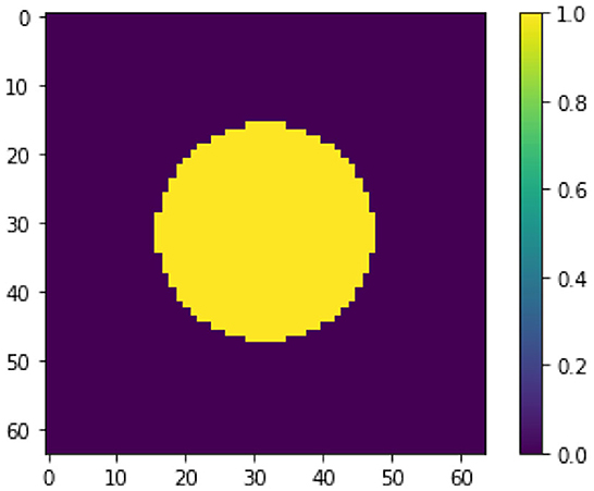
Figure 1. Groundtruth image x^† of a circle.

A first attempt to solve this ill-posed perceptron inversion problem is via Landweber regularization [52]. In Figure 2, we see the reconstructed image obtained with Landweber regularization in combination with early stopping following Morozov's discrepancy principle [22, 53]. Even though the Landweber regularized reconstruction matches the data up to the discrepancy value ||σ(Wx^K + b) − y^δ||, the recovered image does not resemble the image x^†. We will discuss shortly the reason for this visually poor inversion. In comparison, we see a regularized inversion via the total variation regularization approach following (14) in Figure 3. The regularization parameter for this reconstruction is chosen as α = 1.5 × 10⁻². Both x₀ and z are initialized with zero vectors. The stepsize-parameters are chosen as ${\tau }_x=1.99/||W{||}_2^2$ and τ_z = 1/(8α), see [54]. We stop the iterations when changes in x₀ and z in norm are less than a threshold of 10⁻⁵ or when we reach the maximum number of iterations, which we set to 10, 000. As shown in Figure 3, the TV-regularization approach is capable of finding a (visually) more meaningful solution.

FIGURE 2

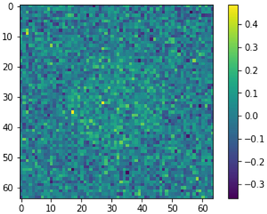
Figure 2. Inverted image via Landweber regularization.

FIGURE 3

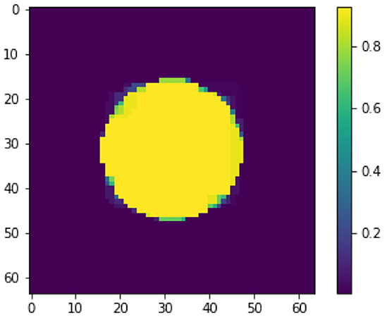
Figure 3. Inverted image via TV regularization.

To explain why the Landweber iteration performs worse compared to the total variation regularization for this specific example, we compare the ℓ₂ norms of each two solutions and the groundtruth image x^†. The ℓ₂ norm of the Landweber solution in Figure 2 measures 6.58 while the TV-regularized solution as in Figure 3 and the groundtruth image x^† measure 25.69 and 28.07, respectively. This is not surprising, as the Landweber iteration is known to converge to a minimal Euclidean norm solution if the noise level converges to zero. On the other hand, when we compare the TV semi-norm of each solution, the groundtruth image in measures 128.0, while the Landweber solution in Figure 2 and TV-regularized solution in Figure 3 measure 707.02 and 114.93, respectively, suggesting that the TV-semi-norm is a more suitable regularization function for the inversion of cartoon-like images such as x^†.

5.1.2. MNIST

In this second example, we perform perceptron inversion on the MNIST dataset [51]. In particular, we consider the following experimental setup. We first train an autoencoder $\mathcal{A}(x)=\mathcal{D}[ℰ(x,{\Theta }_{ℰ}),{\Theta }_{\mathcal{D}}]$, where $\mathcal{D}(·,{\Theta }_{\mathcal{D}})$ and $ℰ(·,{\Theta }_{ℰ})$ denotes the decoder and the encoder, parameterized by parameters ${\Theta }_{\mathcal{D}}$ and ${\Theta }_{\mathcal{E}}$, respectively. We pre-train the autoencoder $\mathcal{A}$, compute the code $ℰ(x,{\Theta }_{ℰ})$ and assign it to the noise-free data variable y, and solve the inverse problem for the input x from the perturbed code y^δ

$\begin{array}{l}\mathcal{E}\left(x,{\Theta }_{\mathcal{E}}\right)=y^{\delta }.\end{array}$

To be more precise, we first train a two-layer fully connected autoencoder $\tilde{x}=W_2\left[\sigma (W_{1}x+b_1)\right]+b_2$ using the vanilla stochastic gradient method (SGM) by minimizing the mean squared error (MSE) on the MNIST training dataset. We set the code dimension to 100 and use ReLU as the activation function. Hence ${\Theta }_{\mathcal{E}}=(W_1,b_1)$ where $W_1\in {ℝ}^{784\times 100}$ and $b_1\in {ℝ}^{100\times 1}$.

We then invert the code $y^{\delta }=\sigma (W_{1}x+b_1)$ via (11) with Equation (14). All MNIST images are centered as a means of pre-processing. The stepsize-parameters are chosen at ${\tau }_x=1.99/||W_1|{|}_2^2$ and τ_z = 1/(8α). We choose the regularization parameter α in the range [10⁻⁴, 10⁻²] and set to 5 × 10⁻³ for all sample images from the training set, and to α = 5 × 10⁻² for all sample images from the validation set. These choices work well with regards to the visual quality of the inverted images.

In Figure 4, we show visualizations of five sample images from the training set, and from the validation set respectively. In comparison, we have also visualized the decoder output. As can be seen, using the code that contains the same compressed information, the inverted images show more clearly defined edges and better visual quality than the decoded outputs. This is to be expected as we compare a nonlinear regularized inversion method with a linear decoder.

FIGURE 4

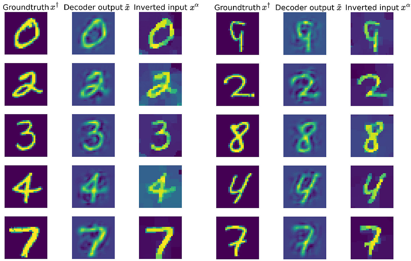
Figure 4. Groundtruth input images from the MNIST training dataset (Left) and validation dataset (Right), together with the corresponding autoencoder output images $\tilde{x}$ and inversions x^α of the encoding via (11).

5.2. Multi-layer perceptrons

In this section, we present numerical results for inverting multi-layer perceptrons. In particular, we consider feedforward neural networks with convolutional layers (CNN), where in the network architecture two-dimensional convolution operations are used to represent the linear operations in the affine-linear functions f(x, Θ). Similar to the experimental design described in Section 5.1, we consider a multi-layer neural network inversion problem where we infer input image x from a noise perturbed code y^δ.

More specifically, we first train a six-layer convolutional autoencoder on the MNIST training dataset via stochastic gradient method to minimize the MSE. The encoder $\mathcal{E}(x,{\Theta }_{\mathcal{E}})$ consists of two convolutional layers, both with 4 × 4 convolutions with stride 2, each followed by the application of a ReLU activation function. As image spatial dimension reduces by half, we double the number of feature channels from 8 to 16. We use a fully-connected layer with weights $W_3\in {ℝ}^{300\times 784}$ and bias $b_3\in {ℝ}^{300\times 1}$ to generate the code. The decoder network first expands the code with an affine-linear transformation with weights $W_4\in {ℝ}^{784\times 300}$ and bias $b_4\in {ℝ}^{784\times 1}$. This is followed by two layers of transpose convolutions with kernel size 4 × 4, where each is followed by a ReLU activation function. The number of feature channels halves each time as we double the spatial dimension.

Following the implementation details outlined in Section 4.2, we iteratively compute the update steps (16) and (17) to recover x from $y=\mathcal{E}(x,\Theta )$. For the PDHG method, we choose the stepsize-parameters as ${\tau }_x=1.99/||W_1{||}_2^2$ and τ_z = 1/(8α). The initial values x₀ and z are both zero. The update steps stop either after reaching the maximum iterations of 1, 500 or when the improvements on x₀ and z are < 10⁻⁵ in norm. For the coordinate descent algorithm, the stepsize-parameters are set to ${\tau }_{x_l}=1.99/||W_{l+1}{||}^2$ for each layer, where ||·|| denotes the spectral norm.

In Figure 5, we visualize the inverted images, the decoder output images, along with the groundtruth images, from the training dataset and validation dataset, respectively. For each image, α is chosen in the range [10⁻⁴, 10⁻²] and set at 9 × 10⁻³ for both training sample images and validation sample images for best visual inversion quality.

FIGURE 5

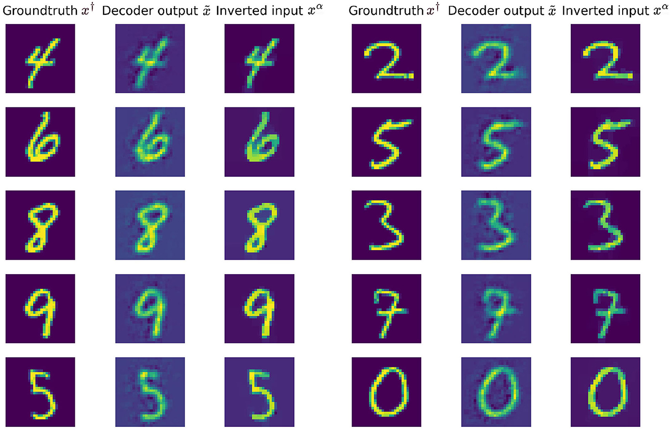
Figure 5. Groundtruth input images from the MNIST training dataset (Left) and validation dataset (Right), together with the corresponding CNN autoencoder output images $\tilde{x}$ and inversions x^α of the encoding via (3).

In Figure 6, we further compare how total variation regularization and decoder respond to different levels of data noise. The noisy data is produced by adding Gaussian noise to perturb the code of each image. We start with zero mean Gaussian noise with standard deviation 0.33 and gradually reduce the noise level, this translates to decreasing δ² from 6.80 down to 0.00.

FIGURE 6

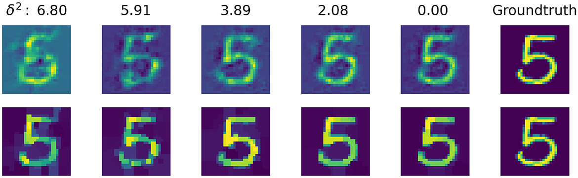
Figure 6. Visualization of the comparison between inverted image and decoded image against various levels of noise. (Top) Decoded output image from the trained convolutional autoencoder. (Bottom) Inverted input image from the CNN with total variation regularization.

Please note that for each noise level the regularization factor α is manually selected in the range [10⁻⁴, 10⁻²] for the best PSNR value. As we can see, for the noise level with standard deviation 0.33 where δ² is at 6.80, the decoder is only capable of producing a blurry distorted output, while the inverted image shows the structure of the digit more clearly. When we decrease the noise level down to 0.00, the inverted image becomes more clean-cut while the decoded image is still less sharply defined.

Figure 7 plots the PSNR value of the decoded and inverted image against decreasing noise level. We want to emphasize that it would be more rigorous to compute and compare $D_R^{\mathrm{\text{symm}}}(x_{\alpha (\delta )},x^{†})$ as suggested in the error estimate bound in (9), but empirically the PSNR value does also support the notion of a convergent regularization.

FIGURE 7

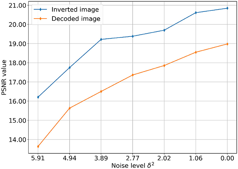
Figure 7. Comparison of PSNR values of total variation-based reconstruction and decoder output per noise level. Each curve reports the change of PSNR value over gradually decreasing levels of Gaussian noise, with δ² ranging from 0.00 to 6.80.

6. Conclusions and outlook

We have introduced a novel variational regularization framework based on a lifted Bregman formulation for the stable inversion of feed-forward neural networks (also known as multi-layer perceptrons). We have proven that the proposed framework is a convergent regularization for the single-layer perceptron case under the mild assumption that the inverse problem solution has to be in the range of the regularization operator. We have derived a general error estimate as well as a specific error estimate for the case that the activation function is the ReLU activation function. We have also addressed the extension of the theory to the multi-layer perceptron case, which can be carried out sequentially, albeit under unrealistic assumptions. We have discussed implementation strategies to solve the proposed scheme computationally, and presented numerical results for the regularized inversion of the image of a circle and piecewise constant images of hand-written digits from single- and multi-layer perceptron outputs with total variation regularization.

Despite all the positive achievements presented in this work, the proposed framework also has some limitations. The framework is currently restricted to feed-forward architectures with affine-linear transformations and proximal activation functions. While it is straight-forward to extend the framework to other architectures such as ResNets [55] or U-Nets [56], it is not straight-forward to include nonlinear operations that cannot be expressed as proximal maps of convex functions, such as max-pooling. However, for many examples there exist remedies, such as using average pooling instead of max-pooling in the previous example.

An open question is how a convergence theory without restrictive, unrealistic assumptions can be established for the multi-layer case. One issue is the non-convexity of the proposed formulation. A remedy could be the use of different architectures that lead to lifted Bregman formulations that are jointly convex in all auxiliary variables.

And last but not least, one would also like to consider other forms of regularization, such as iterative regularization, data-driven regularizations [57], or even combinations of both [58]. However, a convergence analysis for such approaches is currently an open problem.

Data availability statement

Publicly available datasets were analyzed in this study. This data can be found at: http://yann.lecun.com/exdb/mnist/. The programming code for this study can be found in the University of Cambridge data repository at https://doi.org/10.17863/CAM.94404.

Author contributions

XW has programmed and contributed all numerical results as well as Sections 4 and 5. MB has contributed the introduction (Section 1) as well as the theoretical results (Section 3). XW and MB have contributed equally to Sections 2 and 6. Both authors contributed to the article and approved the submitted version.

Funding

The authors acknowledge support from the Cantab Capital Institute for the Mathematics of Information, the Cambridge Centre for Analysis (CCA), and the Alan Turing Institute (ATI).

Conflict of interest

The authors declare that the research was conducted in the absence of any commercial or financial relationships that could be construed as a potential conflict of interest.

Publisher's note

All claims expressed in this article are solely those of the authors and do not necessarily represent those of their affiliated organizations, or those of the publisher, the editors and the reviewers. Any product that may be evaluated in this article, or claim that may be made by its manufacturer, is not guaranteed or endorsed by the publisher.

References

1. LeCun Y, Bengio Y, Hinton G. Deep learning. Nature. (2015) 521:436–44. doi: 10.1038/nature14539

PubMed Abstract | CrossRef Full Text | Google Scholar

2. Goodfellow I, Bengio Y, Courville A. Deep Learning. MIT Press (2016).

Google Scholar

3. Simonyan K, Vedaldi A, Zisserman A. Deep inside convolutional networks: Visualising image classification models and saliency maps. In: Proceedings of the International Conference on Learning Representations (2014). p. 1–8.

4. Fong RC, Vedaldi A. Interpretable explanations of black boxes by meaningful perturbation. In: Proceedings of the IEEE International Conference on Computer Vision. (2017). p. 3429–37. doi: 10.1109/ICCV.2017.371

CrossRef Full Text | Google Scholar

5. Chang CH, Creager E, Goldenberg A, Duvenaud D. Explaining image classifiers by counterfactual generation. arXiv [Preprint]. (2019). arXiv: 1807.08024. Available online at: https://arxiv.org/pdf/1807.08024.pdf

Google Scholar

6. Fong R, Patrick M, Vedaldi A. Understanding deep networks via extremal perturbations and smooth masks. In: Proceedings of the IEEE/CVF International Conference on Computer Vision. (2019). p. 2950–8. doi: 10.1109/ICCV.2019.00304

CrossRef Full Text | Google Scholar

7. Mahendran A, Vedaldi A. Understanding deep image representations by inverting them. In: Proceedings of the IEEE Conference on Computer Vision and Pattern Recognition. (2015). p. 5188–96. doi: 10.1109/CVPR.2015.7299155

PubMed Abstract | CrossRef Full Text | Google Scholar

8. Linden A, Kindermann J. Inversion of multilayer nets. In: Proceedings of International Joint Conference on Neural Networks. Vol. 2 (1989). p. 425–30. doi: 10.1109/IJCNN.1989.118277

CrossRef Full Text | Google Scholar

9. Kindermann J, Linden A. Inversion of neural networks by gradient descent. Parallel Comput. (1990) 14:277–86. doi: 10.1016/0167-8191(90)90081-J

CrossRef Full Text | Google Scholar

10. Jensen CA, Reed RD, Marks RJ, El-Sharkawi MA, Jung JB, Miyamoto RT, et al. Inversion of feedforward neural networks: algorithms and applications. Proc IEEE. (1999) 87:1536–49. doi: 10.1109/5.784232

CrossRef Full Text | Google Scholar

11. Lu BL, Kita H, Nishikawa Y. Inverting feedforward neural networks using linear and nonlinear programming. IEEE Trans Neural Netw. (1999) 10:1271–90. doi: 10.1109/72.809074

PubMed Abstract | CrossRef Full Text | Google Scholar

12. Kingma DP, Welling M. Auto-encoding variational Bayes. arXiv preprint arXiv:13126114. (2013).

PubMed Abstract | Google Scholar

13. Rezende D, Mohamed S. Variational inference with normalizing flows. In: International Conference on Machine Learning. (2015). p. 1530–8.

Google Scholar

14. Dinh L, Krueger D, Bengio Y. Nice: Non-linear independent components estimation. In: International Conference on Learning Representations (2015).

Google Scholar

15. Zhu JY, Park T, Isola P, Efros AA. Unpaired image-to-image translation using cycle-consistent adversarial networks. In: Proceedings of the IEEE International Conference on Computer Vision. (2017). p. 2223–32. doi: 10.1109/ICCV.2017.244

CrossRef Full Text | Google Scholar

16. Sohl-Dickstein J, Weiss E, Maheswaranathan N, Ganguli S. Deep unsupervised learning using nonequilibrium thermodynamics. In: International Conference on Machine Learning. (2015). p. 2256–65.

Google Scholar

17. Ho J, Jain A, Abbeel P. Denoising diffusion probabilistic models. Adv Neural Inform Process Syst. (2020) 33:6840–51.

Google Scholar

18. Behrmann J, Grathwohl W, Chen RT, Duvenaud D, Jacobsen JH. Invertible residual networks. In: International Conference on Machine Learning. (2019). p. 573–82.

Google Scholar

19. Behrmann J, Vicol P, Wang KC, Grosse R, Jacobsen JH. Understanding and mitigating exploding inverses in invertible neural networks. In: International Conference on Artificial Intelligence and Statistics. (2021). p. 1792–800.

Google Scholar

20. Xia W, Zhang Y, Yang Y, Xue JH, Zhou B, Yang MH. GAN inversion: a survey. IEEE Trans Pattern Anal Mach Intell. (2022) 45:3121–38. doi: 10.1109/TPAMI.2022.3181070

PubMed Abstract | CrossRef Full Text | Google Scholar

21. Gal R, Alaluf Y, Atzmon Y, Patashnik O, Bermano AH, Chechik G, et al. An image is worth one word: Personalizing text-to-image generation using textual inversion. arXiv preprint arXiv:220801618. (2022).

Google Scholar

22. Engl HW, Hanke M, Neubauer A. Regularization of Inverse Problems. Vol. 375. Springer Science & Business Media (1996). doi: 10.1007/978-94-009-1740-8

CrossRef Full Text | Google Scholar

23. Scherzer O, Grasmair M, Grossauer H, Haltmeier M, Lenzen F. Variational Methods in Imaging. (2009). doi: 10.1007/978-0-387-69277-7

CrossRef Full Text | Google Scholar

24. Benning M, Burger M. Modern regularization methods for inverse problems. Acta Numer. (2018) 27:1–111. doi: 10.1017/S0962492918000016

CrossRef Full Text | Google Scholar

25. Lunz S, Öktem O, Schönlieb CB. Adversarial regularizers in inverse problems. In: Advances in Neural Information Processing Systems. (2018). p. 31.

Google Scholar

26. Arridge S, Maass P, Öktem O, Schönlieb CB. Solving inverse problems using data-driven models. Acta Numer. (2019) 28:1–174. doi: 10.1017/S0962492919000059

CrossRef Full Text | Google Scholar

27. Schwab J, Antholzer S, Haltmeier M. Deep null space learning for inverse problems: convergence analysis and rates. Inverse Probl. (2019) 35:025008. doi: 10.1088/1361-6420/aaf14a

PubMed Abstract | CrossRef Full Text | Google Scholar

28. Li H, Schwab J, Antholzer S, Haltmeier M. NETT: Solving inverse problems with deep neural networks. Inverse Probl. (2020) 36:065005. doi: 10.1088/1361-6420/ab6d57

CrossRef Full Text | Google Scholar

29. Mukherjee S, Dittmer S, Shumaylov Z, Lunz S, Öktem O, Schönlieb CB. Learned convex regularizers for inverse problems. arXiv preprint arXiv:200802839v2. (2021).

Google Scholar

30. Wang X, Benning M. Lifted Bregman training of neural networks. arXiv preprint arXiv:220808772. (2022).

Google Scholar

31. Wang X, Benning M. Generalised perceptron learning. In: 12th Annual Workshop on Optimization for Machine Learning. (2020). Available online at: https://opt-ml.org/papers/2020/paper_68.pdf

Google Scholar

32. Bregman LM. The relaxation method of finding the common point of convex sets and its application to the solution of problems in convex programming. USSR Comput Math Math Phys. (1967) 7:200–17. doi: 10.1016/0041-5553(67)90040-7

CrossRef Full Text | Google Scholar

33. Kiwiel KC. Proximal minimization methods with generalized Bregman functions. SIAM J Control Optim. (1997) 35:1142–68. doi: 10.1137/S0363012995281742

CrossRef Full Text | Google Scholar

34. Lin J. Divergence measures based on the Shannon entropy. IEEE Trans Inform Theory. (1991) 37:145–51. doi: 10.1109/18.61115

CrossRef Full Text | Google Scholar

35. Burbea J, Rao C. On the convexity of higher order Jensen differences based on entropy functions (Corresp.). IEEE Trans Inform Theory. (1982) 28:961–3. doi: 10.1109/TIT.1982.1056573

CrossRef Full Text | Google Scholar

36. Burbea J, Rao C. On the convexity of some divergence measures based on entropy functions. IEEE Trans Inform Theory. (1982) 28:489–95. doi: 10.1109/TIT.1982.1056497

CrossRef Full Text | Google Scholar

37. Nielsen F, Boltz S. The burbea-rao and bhattacharyya centroids. IEEE Trans Inform Theory. (2011) 57:5455–66. doi: 10.1109/TIT.2011.2159046

CrossRef Full Text | Google Scholar

38. Beck A. First-order methods in optimization. SIAM. (2017). doi: 10.1137/1.9781611974997

CrossRef Full Text | Google Scholar

39. Benning M, Burger M. Error estimates for general fidelities. Electron Trans Numer Anal. (2011) 38:77.

Google Scholar

40. Chambolle A, Pock T. An introduction to continuous optimization for imaging. Acta Numer. (2016) 25:161–319. doi: 10.1017/S096249291600009X

CrossRef Full Text | Google Scholar

41. Zhu M, Chan T. An efficient primal-dual hybrid gradient algorithm for total variation image restoration. Ucla Cam Rep. (2008) 34:8–34.

Google Scholar

42. Pock T, Cremers D, Bischof H, Chambolle A. An algorithm for minimizing the Mumford-Shah functional. In: 2009 IEEE 12th International Conference on Computer Vision. (2009). p. 1133–40. doi: 10.1109/ICCV.2009.5459348

CrossRef Full Text | Google Scholar

43. Esser E, Zhang X, Chan TF. A general framework for a class of first order primal-dual algorithms for convex optimization in imaging science. SIAM J Imaging Sci. (2010) 3:1015–46. doi: 10.1137/09076934X

CrossRef Full Text | Google Scholar

44. Chambolle A, Pock T. A first-order primal-dual algorithm for convex problems with applications to imaging. J Math Imaging Vis. (2011) 40:120–45. doi: 10.1007/s10851-010-0251-1

CrossRef Full Text | Google Scholar

45. Benning M, Riis ES. Bregman methods for large-scale optimization with applications in imaging. In: Chen K, Schönlieb CB, Tai XC, Younces L, editors. Handbook of Mathematical Models and Algorithms in Computer Vision and Imaging. Cham: Springer (2023). doi: 10.1007/978-3-030-03009-4_62-2

CrossRef Full Text | Google Scholar

46. Rudin LI, Osher S, Fatemi E. Nonlinear total variation based noise removal algorithms. Phys D. (1992) 60:259–68. doi: 10.1016/0167-2789(92)90242-F

CrossRef Full Text | Google Scholar

47. Chambolle A, Lions PL. Image recovery via total variation minimization and related problems. Numer Math. (1997) 76:167–88. doi: 10.1007/s002110050258

CrossRef Full Text | Google Scholar

48. Beck A, Tetruashvili L. On the convergence of block coordinate descent type methods. SIAM J Optim. (2013) 23:2037–60. doi: 10.1137/120887679

PubMed Abstract | CrossRef Full Text | Google Scholar

49. Wright SJ. Coordinate descent algorithms. Math Programm. (2015) 151:3–34. doi: 10.1007/s10107-015-0892-3

CrossRef Full Text | Google Scholar

50. Wright SJ, Recht B. Optimization for Data Analysis. Cambridge University Press (2022). doi: 10.1017/9781009004282

CrossRef Full Text | Google Scholar

51. LeCun Y, Bottou L, Bengio Y, Haffner P. Gradient-based learning applied to document recognition. Proc IEEE. (1998) 86:2278–324. doi: 10.1109/5.726791

CrossRef Full Text | Google Scholar

52. Landweber L. An iteration formula for Fredholm integral equations of the first kind. Am J Math. (1951) 73:615–24. doi: 10.2307/2372313

CrossRef Full Text | Google Scholar

53. Morozov VA. Methods for Solving Incorrectly Posed Problems. Springer Science & Business Media (2012).

Google Scholar

54. Chambolle A. An algorithm for total variation minimization and applications. J Math Imaging Vis. (2004) 20:89–97. doi: 10.1023/B:JMIV.0000011321.19549.88

PubMed Abstract | CrossRef Full Text | Google Scholar

55. He K, Zhang X, Ren S, Sun J. Deep residual learning for image recognition. In: Proceedings of the IEEE Conference on Computer Vision and Pattern Recognition. (2016). p. 770–8. doi: 10.1109/CVPR.2016.90

PubMed Abstract | CrossRef Full Text | Google Scholar

56. Ronneberger O, Fischer P, Brox T. U-net: convolutional networks for biomedical image segmentation. In: Medical Image Computing and Computer-Assisted Intervention-MICCAI 2015: 18th International Conference. Munich: Springer (2015). p. 234–41. doi: 10.1007/978-3-319-24574-4_28

CrossRef Full Text | Google Scholar

57. Kabri S, Auras A, Riccio D, Bauermeister H, Benning M, Moeller M, et al. Convergent data-driven regularizations for CT reconstruction. arXiv [Preprint]. (2022). arXiv: 2212.07786. Available online at: https://arxiv.org/pdf/2212.07786.pdf

PubMed Abstract | Google Scholar

58. Aspri A, Banert S, Öktem O, Scherzer O. A data-driven iteratively regularized Landweber iteration. Numer Funct Anal Optim. (2020) 41:1190–227. doi: 10.1080/01630563.2020.1740734

CrossRef Full Text | Google Scholar