A combination of physics-informed neural networks with the fixed-stress splitting iteration for solving Biot's model

1. Introduction

Biot's consolidation model in poroelasticity describes the interaction between fluid flow and the porous structure it saturates. This model was first proposed by Biot [1], and has a wide range of applications, including biomechanics [2] and petroleum engineering [3]. The partial differential equations (PDEs) for the quasi-static Biot system in a bounded domain Ω ⊂ ℝ^d (where d = 2 or 3) over the time interval (0, T] are as follows:

$\begin{array}{ll}{\partial }_t\left(\frac{1}{M}p+\alpha \nabla ·u\right)-\nabla ·K\nabla p=f\text{in Ω}\times (0,T],& (1)\end{array}$

$\begin{array}{ll}-\nabla ·\sigma (u)+\alpha \nabla p=g\text{in Ω}\times (0,T].& (2)\end{array}$

Here, u is the displacement of solid, p is the fluid pressure, g is the body force, f is a source or sink term, σ(u) = 2με(u) + λdivuI with $\epsilon (u)=\frac{1}{2}\left[\nabla u+{(\nabla u)}^T\right]$ being the strain tensor. The Lamé constants λ and μ are expressed in terms of the Young's modulus E and the Poisson ratio ν as

$\begin{array}{ll}\text{λ}=\frac{E\nu }{(1+\nu )(1-2\nu )},\mu =\frac{E}{2(1+\nu )}.& (3)\end{array}$

Other physical parameters are the Biot-Willis constant α > 0, which is close to 1, Biot's modulus M > 0, and hydraulic conductivity K. Equation (1) represents the mass conservation and Equation (2) means forces balance. For ease of presentation, we assume the following pure Dirichlet conditions.

$\begin{array}{ll}u=u_d,p=p_d\text{on }\partial \text{Ω}\times (0,T].& (4)\end{array}$

The initial conditions are

$\begin{array}{ll}u=u_0,p=p_0\text{in Ω}\times \left\{0\right\}.& (5)\end{array}$

The discussion of the existence and uniqueness of the solution of Biot's system (1)–(5) can be found in [4–6]. In this work, we focus on the algorithm aspect.

Several classical numerical methods have been proposed to solve this problem, including finite volume methods [7], virtual element methods [8], and mixed finite element methods [9]. Biot's model is a multiphysics problem involving both linear elasticity and porous media flow. Numerical difficulties such as elastic locking and pressure oscillations can arise, especially for models based on two-field formulations [10–13]. To overcome these difficulties, various methods have been proposed, such as the discontinuous Galerkin method [14], stabilized finite element methods [11, 15], and three-field or four-field reformulations using inf-sup stable finite element pairs [12, 16–18]. These methods may face challenges in terms of large computational overhead. The fixed-stress splitting iterative method [19, 20] is proposed to address this issue. This method breaks down the original problem into two subproblems and solves them in an iterative manner, rather than solving the entire system at once. The method relies on the contraction mapping principle to prove its convergence [19] and has been shown to be efficient through various studies. Further studies have been carried out based on the fixed-stress splitting iterative method, such as the analysis of the relationship between the convergence rate and the stabilization parameter [21–23] and the implementation of a parallel-in-time strategy to speed up the computations [24].

In recent years, deep neural networks (DNNs) have demonstrated impressive potential in solving partial differential equations (PDEs) with a wide range of applications in various domains. Among DNNs, physics-informed neural networks (PINNs) have become a popular class due to their ability to solve PDEs without meshing. PINNs have proven successful in solving high-dimensional problems and interface problems, and they can tackle inverse problems with slight modifications of the loss function [25–27]. Several studies have used PINNs to tackle the Biot's model [28–30], where the key advantage of PINNs over traditional methods such as finite element methods is their ability to avoid numerical difficulties arising from meshing and not requiring inf-sup stability. Therefore, from a flexibility perspective, deep neural network methods are preferable. However, most of these studies employ a monolithic approach to train the neural network solution, with only one study using a sequential training approach [27], which lacks theoretical analysis and only presents numerical experiments. In this paper, we propose a combination of physics-informed neural networks with fixed-stress splitting method (FS-PINNs) to solve Biot's equations. We employ two PINNs and incorporate them into the fixed-stress splitting iterative method. Our method involves two separate neural networks, one for solid displacement and another for fluid pressure, leading to faster convergence and lower computational cost than classical PINNs [31, 32]. Through a detailed analysis of the monotonic convergence of the fixed-stress splitting method, we present an error estimate for the solution of the proposed FS-PINNs. Future work could include refining the neural network architecture to improve the accuracy and further reduce the computational cost. In addition, the potential application of our approach to other PDE problems and multiphysics problems could be explored. Overall, the proposed FS-PINNs represent a promising approach for solving poroelastic models with faster convergence and lower computational cost.

The remaining sections of the paper are organized as follows. Section 2 provides an overview of the fixed-stress splitting iterative method for Biot's model. In Section 3, we introduce the fixed-stress splitting iterative PINNs (FS-PINNs) and present theoretical analyses to demonstrate their approximation properties. Section 4 presents numerical experiments to demonstrate the effectiveness of the proposed method. Finally, conclusions are drawn in Section 5.

2. Fixed-stress splitting method for Biot's equations

In this section, we introduce an iterative scheme proposed in [19], called the fixed-stress splitting method. Instead of solving Biot's model (1)–(5) in a monolithic way, this method decouples the original problem into two subproblems and solves them in an iterative manner. Given a large enough stabilization parameter β_FS and an initial guess (p⁰, u⁰), the standard fixed-stress splitting method computes a sequence of approximations as follows:

The first step: Given pⁿ and uⁿ, we solve for pⁿ⁺¹ satisfying

$\begin{array}{l}\left(\frac{1}{M}+{\beta }_{FS}\right){\partial }_t{p}^{n+1}-\nabla ·K\nabla p^{n+1}=\\ f-\alpha \nabla ·{\partial }_t{u}^n+{\beta }_{FS}{\partial }_t{p}^n\text{in Ω}\times (0,T],& (6)\end{array}$

$\begin{array}{ll}{p}^{n+1}=p_0\text{in Ω}\times \left\{0\right\},& (7)\end{array}$

$\begin{array}{ll}{p}^{n+1}=p_d\text{on }\partial \text{Ω}\times (0,T].& (8)\end{array}$

The second step: Using pⁿ⁺¹, we solve for uⁿ⁺¹ satisfying

$\begin{array}{ll}-\nabla ·\sigma (u^{n+1})=g-\alpha \nabla p^{n+1}\text{in Ω}\times (0,T],& (9)\end{array}$

$\begin{array}{ll}{u}^{n+1}=u_0\text{in Ω}\times \left\{0\right\},& (10)\end{array}$

$\begin{array}{ll}{u}^{n+1}=u_d\text{on }\partial \text{Ω}\times (0,T].& (11)\end{array}$

To derive the variational formulation of the fixed-stress problem (6)–(11), we define the proper functional spaces with H¹(Ω) denoting the Hilbert subspace as follows.

$\begin{array}{l}W=\{p\in H^1([0,T];H^1(\text{Ω}))|p{|}_{\partial \text{Ω}}=p_d\},\\ V=\{u\in H^1([0,T];H^1(\text{Ω}))|u{|}_{\partial \text{Ω}}=u_d\}.\end{array}$

Multiplying (6), (9) by test functions, and applying the integration by parts, we obtain the variational problems: for a given t ≥ 0, find {(p^{n + 1}, u^{n + 1})} ⊂ W × V such that

$\begin{array}{l}\left(\frac{1}{M}+{\beta }_{FS}\right){\displaystyle {\int }_{\text{Ω}}({\partial }_t{p}^{n+1})}\psi dx+K{\displaystyle {\int }_{\text{Ω}}(\nabla p^{n+1})(\nabla \psi )}dx\\ ={\displaystyle {\int }_{\text{Ω}}f}\psi dx-\alpha {\displaystyle {\int }_{\text{Ω}}(\nabla ·{\partial }_t{u}^n)}\psi dx+{\beta }_{FS}{\displaystyle {\int }_{\text{Ω}}({\partial }_t{p}^n)}\psi dx,\forall \psi \in W,& (12)\end{array}$

$\begin{array}{l}2\mu {\displaystyle {\int }_{\text{Ω}}\epsilon }(u^{n+1}):\epsilon (v)dx+\text{λ}{\displaystyle {\int }_{\text{Ω}}(\nabla ·u^{n+1})(\nabla ·v)}dx\\ ={\displaystyle {\int }_{\text{Ω}}gvdx}+\alpha {\displaystyle {\int }_{\text{Ω}}(\nabla ·v)}{p}^{n+1}dx,\forall v\in V.& (13)\end{array}$

Assume that (p, u) ∈ W × V is the unique solution of Biot's system (1)–(5). Given a large enough stabilization parameter β_FS, the sequence {(pⁿ⁺¹, uⁿ⁺¹)} ⊂ W × V generated by Equations (12, 13) converges to the solution (p, u). More precisely, we can state the following:

THEOREM 2.1. The sequence {(pⁿ⁺¹, uⁿ⁺¹)} ⊂ W × V generated by Equations (6)–(11) converges to (p, u) ∈ W × V for any ${\beta }_{FS}\ge \frac{{\alpha }^2}{2\left(\frac{2\mu }{d}+\text{λ}\right)}$. If one denotes $e_u^{n+1}:\; =u^{n+1}-u$ and $e_p^{n+1}:\; =p^{n+1}-p$, then there holds

$\begin{array}{ll}{\displaystyle {\int }_0^T{\displaystyle {\int }_{\text{Ω}}{({\partial }_t{e}_p^{n+1})}^2}}dxdt\le L{\displaystyle {\int }_0^T{\displaystyle {\int }_{\text{Ω}}{({\partial }_t{e}_p^n)}^2}}dxdt,& (14)\end{array}$

where $L=\frac{{\beta }_{FS}}{{\beta }_{FS}+\frac{2}{M}}$ is a positive constant strictly smaller than 1.

REMARK 2.2. We have included a convergence analysis of the fixed-stress splitting iterative method in the Appendix. In our proof, we demonstrate that the differences $e_p^{n+1}$ and $e_u^{n+1}$ approach zeros as n tends to infinity. Our proof helps to illustrate the convergence of the fixed-stress splitting method.

3. The classical PINNs and the FS-PINNs for solving Biot's model

In this section, we introduce the training procedure of the classical PINNs for solving Biot's model, and propose an iterative deep learning method combining the fixed-stress splitting method, called FS-PINNs. The proposed FS-PINNs consist of two independent PINNs, one for pressure, and the other for displacement. We then present the training procedure and a theoretical analysis of the proposed FS-PINNs.

3.1. Training procedure of the classical PINNs

The idea of using the classical PINNs to solve PDEs is from [25], which can be easily extended to solve Biot's model. The main idea is to design loss functions for fully connected neural networks. In this context, we provide a brief overview of the training procedure for solving problem (1)–(5), which is illustrated in Figure 1.

FIGURE 1

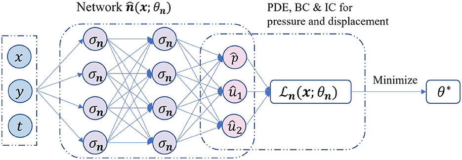
Figure 1. The training procedure of the classical PINNs using unified activation functions for a 2D Biot's model.

The functional form of a classical PINN is given as follows.

$\begin{array}{ll}\widehat{n}(x;{\theta }_n)=(\widehat{p}(x;{\theta }_n);\widehat{u}(x;{\theta }_n))={\text{Σ}}_n^{L_n}◦{\text{Σ}}_n^{L_n-1}◦\cdots ◦{\text{Σ}}_n^1(x).& (15)\end{array}$

Here, $\widehat{n}$ is the network approximation of the exact solution (p; u) with L_n hidden layers with the input $x=(x_1,\cdots ,x_d,t)\in {ℝ}^d\times \left[0,T\right]$. The collection of parameter θ_n is given by

$\begin{array}{ll}{\theta }_n=\{W_n^1,W_n^2,\cdots ,W_n^{L_n},b_n^1,b_n^2,\cdots ,b_n^{L_n}\}.& (16)\end{array}$

The mapping function ${\text{Σ}}_n^i$ is defined as

$\begin{array}{ll}{x}_n^i:\; ={\text{Σ}}_n^i(x_n^{i-1})={\sigma }_n^i(W_n^i{x}_n^{i-1}+b_n^i),i=1,2,\cdots ,L_n.& (17)\end{array}$

Here, $(W_n^i,b_n^i,{\sigma }_n^i)$ represent the weights, biases, and activation functions of the i-th layer for network $\widehat{n}$. It is assumed that the number of neurons in each hidden layer is set to be the same N_n and that all activation functions ${\sigma }_n^i$ are identical.

After setting up the architecture, we can begin training the parameter θ_n using the procedure:

$\begin{array}{ll}{\theta }^{*}=\underset{{\theta }_n}{\arg \min }{\mathcal{L}}_n(x;{\theta }_n),& (18)\end{array}$

where ${\mathcal{L}}_n$ is the loss function. The loss function for the classical PINNs generally consists of three components: the PDEs loss, the initial condition loss, and the boundary condition loss. The PDEs loss represents the residual of the governing equations, while the initial and boundary condition losses ensure that the predicted solution satisfies the initial and boundary conditions. The loss function is denoted by ${\mathcal{L}}_n(x;{\theta }_n)$ and has the following representation.

$\begin{array}{l}{\mathcal{L}}_n(x;{\theta }_n)=\frac{1}{N_1}{\displaystyle \sum _{i=1}^{N_1}\left({\Vert \widehat{p}(x_1^i;{\theta }_n)-p^i\Vert }_{L^2}^2+{\Vert \widehat{u}(x_1^i;{\theta }_n)-u^i\Vert }_{L^2}^2\right)}\\ +\frac{1}{N_2}{\displaystyle \sum _{i=1}^{N_2}(}\Vert \frac{1}{M}{\partial }_t\widehat{p}(x_2^i;{\theta }_n)-\nabla ·K\nabla \widehat{p}(x_2^i;{\theta }_n)+\\ \alpha \nabla ·{\partial }_t\widehat{u}(x_2^i;{\theta }_n)-f(x_2^i){\Vert }_{L^2}^2+\Vert -\nabla ·\sigma (\widehat{u}(x_2^i;{\theta }_n))+\\ {\alpha \nabla \widehat{p}(x_2^i;{\theta }_n)-g(x_2^i)\Vert }_{L^2}^2).\end{array}$

The above expression uses the mean square error (MSE) to measure errors. In this expression, ${\left\{x_1^i\right\}}_{i=1}^{N_1}$ represents the initial and boundary training data, while ${\left\{x_2^i\right\}}_{i=1}^{N_2}$ represents the collocation points in the domain. We then optimize θ_n to obtain θ^*. For cases involving mixed boundary conditions, one can refer to [28] for more details.

3.2. Training procedure of the proposed FS-PINNs

The primary innovation of our approach is incorporating the fixed-stress strategy into the training procedure of PINNs. The proposed method includes two independent PINNs to solve for displacement and fluid pressure separately. We can then train our FS-PINNs iteratively with respect to their corresponding loss functions. Figure 2 illustrates the training procedure.

FIGURE 2

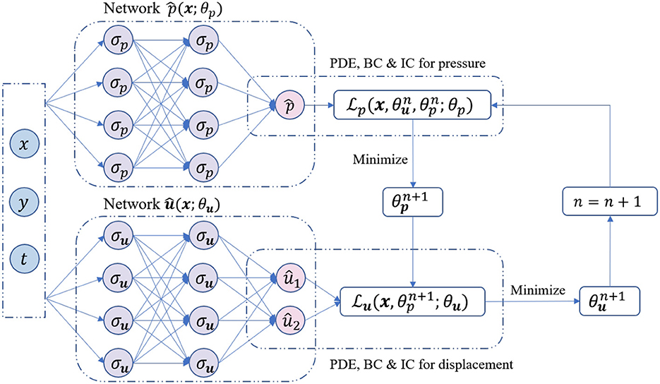
Figure 2. The training procedure of the proposed FS-PINNs. Two independent networks are trained iteratively with respect to the corresponding loss functions.

Similar to the classical PINNs, the functional forms of the two independent PINNs are as follows.

$\begin{array}{ll}\widehat{p}(x;{\theta }_p)={\text{Σ}}_p^{L_p}◦{\text{Σ}}_p^{L_p-1}◦\cdots ◦{\text{Σ}}_p^1(x),& (19)\end{array}$

$\begin{array}{ll}\widehat{u}(x;{\theta }_u)={\text{Σ}}_u^{L_u}◦{\text{Σ}}_u^{L_u-1}◦\cdots ◦{\text{Σ}}_u^1(x).& (20)\end{array}$

Here, $\widehat{p}$ refers to the network approximation of pressure p with L_p hidden layers, while $\widehat{u}$ refers to the network approximation of displacement u with L_u hidden layers. The collection of parameters of $\widehat{p}$ and $\widehat{u}$ are denoted by θ_p and θ_u, respectively, and are given by:

$\begin{array}{ll}{\theta }_p=\{W_p^1,W_p^2,\cdots ,W_p^{L_p},b_p^1,b_p^2,\cdots ,b_p^{L_p}\},& (21)\end{array}$

$\begin{array}{ll}{\theta }_u=\{W_u^1,W_u^2,\cdots ,W_u^{L_u},b_u^1,b_u^2,\cdots ,b_u^{L_u}\}.& (22)\end{array}$

The mapping functions ${\text{Σ}}_p^i$ and ${\text{Σ}}_u^i$ are defined as

$\begin{array}{ll}{x}_p^i:\; ={\text{Σ}}_p^i(x_p^{i-1})={\sigma }_p^i(W_p^i{x}_p^{i-1}+b_p^i),i=1,2,\cdots ,L_p,& (23)\end{array}$

$\begin{array}{ll}{x}_u^i:\; ={\text{Σ}}_u^i(x_u^{i-1})={\sigma }_u^i(W_u^i{x}_u^{i-1}+b_u^i),i=1,2,\cdots ,L_u.& (24)\end{array}$

In this context, $(W_p^i,b_p^i,{\sigma }_p^i)$ and $(W_u^i,b_u^i,{\sigma }_u^i)$ represent the weights, biases, and activation functions of the i-th layer for $\widehat{p}$ and $\widehat{u}$, respectively. It is also assumed that the number of neurons in each hidden layer of $\widehat{p}$ and $\widehat{u}$ is set to N_p and N_u, respectively. Furthermore, all activation functions ${\sigma }_p^i$ and ${\sigma }_u^i$ are assumed to be identical.

From now, our attention turns to developing the loss functions. By utilizing the fixed-stress splitting method detailed in Equations (6)–(8) and Equations (9)–(11), we can impose constraints on the networks $\widehat{p}$ and $\widehat{u}$, respectively. We begin by setting n = 0 and ${\theta }_p^n={\theta }_u^n=0$. We can then formulate the optimization problem as follows. In the first step, we obtain ${\theta }_p^{n+1}$ by solving for the minimum of ${\mathcal{L}}_p(x,{\theta }_u^n,{\theta }_p^n;{\theta }_p)$:

$\begin{array}{ll}{\theta }_p^{n+1}=\underset{{\theta }_p}{\arg \min }{\mathcal{L}}_p(x,{\theta }_u^n,{\theta }_p^n;{\theta }_p).& (25)\end{array}$

In the second step, we obtain ${\theta }_u^{n+1}$ by solving for the minimum of ${\mathcal{L}}_u(x,{\theta }_p^{n+1};{\theta }_u)$:

$\begin{array}{ll}{\theta }_u^{n+1}=\underset{{\theta }_u}{\arg \min }{\mathcal{L}}_u(x,{\theta }_p^{n+1};{\theta }_u).& (26)\end{array}$

To be clear, ${\mathcal{L}}_p$ and ${\mathcal{L}}_u$ denote the loss functions for networks $\widehat{p}$ and $\widehat{u}$, respectively. These loss functions are defined as follows:

$\begin{array}{l}{\mathcal{L}}_p(x,{\theta }_u^n,{\theta }_p^n;{\theta }_p)=\frac{1}{N_3}{\displaystyle \sum _{i=1}^{N_3}{\Vert \widehat{p}(x_p^i;{\theta }_p)-p(x_p^i)\Vert }^2}\\ +\frac{1}{N_4}{\displaystyle \sum _{i=1}^{N_4}\Vert }\left(\frac{1}{M}+{\beta }_{FS}\right){\partial }_t\widehat{p}(x_f^i;{\theta }_p)-\nabla ·K\nabla \widehat{p}(x_f^i;{\theta }_p)\\ +\alpha \nabla ·{\partial }_t\widehat{u}(x_f^i;{\theta }_u^n)-{\beta }_{FS}{\partial }_t\widehat{p}(x_f^i;{\theta }_p^n)-f(x_f^i){\Vert }^2,& (27)\end{array}$

$\begin{array}{l}{\mathcal{L}}_u(x,{\theta }_p^{n+1};{\theta }_u)=\frac{1}{N_5}{\displaystyle \sum _{i=1}^{N_5}{\Vert \widehat{u}(x_u^i;{\theta }_u)-u(x_u^i)\Vert }^2}\\ +\frac{1}{N_6}{\displaystyle \sum _{i=1}^{N_6}{\Vert -\nabla ·\sigma (\widehat{u}(x_g^i;{\theta }_u))+\alpha \nabla \widehat{p}(x_g^i;{\theta }_p^{n+1})-g(x_g^i)\Vert }^2}.& (28)\end{array}$

In the above expressions, ${\left\{x_p^i\right\}}_{i=1}^{N_3}$ and ${\left\{x_u^i\right\}}_{i=1}^{N_5}$ denote the initial and boundary training data on p(x) and u(x), respectively. Additionally, ${\left\{x_f^i\right\}}_{i=1}^{N_4}$ and ${\left\{x_g^i\right\}}_{i=1}^{N_6}$ represent the collocation points for f(x) and g(x) in the domain, respectively. By repeatedly updating θ_p and θ_u using (25) and (26), we can get the network approximations of Biot's model: $\widehat{p}(x;{\theta }_p)$ and $\widehat{u}(x;{\theta }_u)$.

3.3. Analysis of the proposed FS-PINNs

The classical PINNs have shown great potential in solving PDEs, but quantifying their errors remains an open problem [26]. The accuracy of neural network approximation is influenced by various factors, such as network architecture, training data, etc. In this section, we assume that PINNs can solve the two subproblems within a certain error tolerance. We then employ an iterative strategy for the proposed FS-PINNs. It is crucial to consider the possibility of error accumulation and divergence since network approximations can not guarantee convergence of the fixed-stress iteration. To address this issue, we observe that the fixed-stress splitting method, which is essentially equivalent to the fixed-point iterative scheme, has been shown to mitigate error accumulation. Therefore, we present a mathematical analysis to demonstrate the robustness of our proposed FS-PINNs. Given an initial guess $({\widehat{p}}^0,{\widehat{u}}^0)$, we describe the procedures of (25) and (26) as follows.

Step 1: Given ${\widehat{p}}^n$ and ${\widehat{u}}^n$, we employ (25) to obtain a network solution ${\widehat{p}}^{n+1}$ for the following problem.

$\begin{array}{ll}\left(\frac{1}{M}+{\beta }_{FS}\right){\partial }_t{p}^{n+1}-\nabla ·K\nabla p^{n+1}=f-\alpha \nabla ·{\partial }_t{\widehat{u}}^n+{\beta }_{FS}{\partial }_t{\widehat{p}}^n\text{in Ω}\times (0,T],& (29)\end{array}$

$\begin{array}{ll}{p}^{n+1}=p_0\text{in Ω}\times \left\{0\right\},& (30)\end{array}$

$\begin{array}{ll}{p}^{n+1}=p_d\text{on }\partial \text{Ω}\times (0,T].& (31)\end{array}$

The corresponding loss function for ${\widehat{p}}^{n+1}$ imposes the initial condition and the boundary condition in the mean square sense.

Step 2: using ${\widehat{p}}^{n+1}$, we employ (26) to obtain a network solution ${\widehat{u}}^{n+1}$ for the following problem.

$\begin{array}{ll}-\nabla ·\sigma (u^{n+1})=g-\alpha \nabla {\widehat{p}}^{n+1}\text{inΩ}\times (0,T],& (32)\end{array}$

$\begin{array}{ll}{u}^{n+1}=u_0\text{in Ω}\times \left\{0\right\},& (33)\end{array}$

$\begin{array}{ll}{u}^{n+1}=u_d\text{on }\partial \text{Ω}\times (0,T].& (34)\end{array}$

The corresponding loss function for ${\widehat{u}}^{n+1}$ imposes the initial condition and the boundary condition in the mean square sense.

To analyze the numerical errors ${\widehat{p}}^{n+1}-p$ and ${\widehat{u}}^{n+1}-u$, we can express them as the sum of two terms: $({\widehat{p}}^{n+1}-p^{n+1})+(p^{n+1}-p)$ and $({\widehat{u}}^{n+1}-u^{n+1})+(u^{n+1}-u)$, which can be dealt with separately. We assume that the Physics-Informed Neural Networks (PINNs) used to solve Equations (29) and (32) can achieve a certain error tolerance, denoted by δ, for the approximations ${\widehat{p}}^{n+1}$ and ${\widehat{u}}^{n+1}$ obtained in each step. This is expressed as

$\begin{array}{ll}\Vert {\widehat{p}}^{n+1}-p^{n+1}{\Vert }_{H^1([0,T];H^1(\text{Ω}))}\le \delta ,\Vert {\widehat{u}}^{n+1}-u^{n+1}{\Vert }_{H^1([0,T];H^1(\text{Ω}))}\le \delta .& (35)\end{array}$

Such assumptions are reasonable if the neural networks are sufficiently deep and wide [33]. For estimating the terms (pⁿ⁺¹−p) and (uⁿ⁺¹−u), we utilize integration by parts and employ the fixed-stress iterative method to analyze convergence. We then build on Theorem 2.1 to perform mathematical analysis.

THEOREM 3.1. Assume that (p, u) ∈ W × V is the unique solution of the problem (1)–(5). Let $({\widehat{p}}^{n+1},{\widehat{u}}^{n+1})$ be the network approximations of Equations (29)–(34), and (pⁿ⁺¹, uⁿ⁺¹) ∈ W × V be the exact solution of (6)–(11). We define $e_u^{n+1}:\; =u^{n+1}-u$ and $e_p^{n+1}:\; =p^{n+1}-p$. Under the assumption (35) with a positive δ, if β_FS is large enough, then there exists a positive number $\tilde{L}<1$ such that the following estimate holds for all n ≥ 0.

$\begin{array}{ll}{\displaystyle {\int }_0^T{\displaystyle {\int }_{\Omega }{({\partial }_t{e}_p^{n+1})}^2}}dxdt\le \stackrel{\sim }{L}{\displaystyle {\int }_0^T{\displaystyle {\int }_{\Omega }{({\partial }_t{e}_p^n)}^2}}dxdt+C{\delta }^2,& (36)\end{array}$

where C is a positive constant. Moreover, the limit superior exists and satisfies:

$\begin{array}{ll}\underset{n\to \infty }{\lim \sup }{\displaystyle {\int }_0^T{\displaystyle {\int }_{\Omega }{({\partial }_t{e}_p^{n+1})}^2}}dxdt\le C\frac{{\delta }^2}{1-\stackrel{\sim }{L}}.& (37)\end{array}$

Proof. Firstly, we start with the second step of FS-PINNs. We subtract the original Equation (2) from the n-th iteration of (32). For the resulted equation, taking the derivative with respect to t, we obtain

$\begin{array}{ll}-\nabla ·\sigma ({\partial }_t{e}_u^n)=-\alpha \nabla {\partial }_t{e}_p^n+\alpha \nabla ({\partial }_t{p}^n-{\partial }_t{\widehat{p}}^n).& (38)\end{array}$

Multiplying (38) by ${\partial }_t{e}_u^n$, applying the divergence theorem, the Cauchy-Schwarz inequality, and the Poincaré inequality, we shall derive the following inequality with any ϵ₁ > 0.

$\begin{array}{l}2\mu {\displaystyle {\int }_0^T{\displaystyle {\int }_{\text{Ω}}\epsilon }}({\partial }_t{e}_u^n):\epsilon ({\partial }_t{e}_u^n)dxdt+\text{λ}{\displaystyle {\int }_0^T{\displaystyle {\int }_{\text{Ω}}{(\nabla ·{\partial }_t{e}_u^n)}^2}}dxdt\\ =\alpha {\displaystyle {\int }_0^T{\displaystyle {\int }_{\text{Ω}}(\nabla ·{\partial }_t{e}_u^n)({\partial }_t{e}_p^n)}}dxdt+\alpha {\displaystyle {\int }_0^T{\displaystyle {\int }_{\text{Ω}}(\nabla (}}{\partial }_t{\widehat{p}}^n-{\partial }_t{p}^n))({\partial }_t{e}_u^n)dxdt\\ \le \frac{1}{2}\left(\frac{2\mu }{d}+\text{λ}\right){\displaystyle {\int }_0^T{\displaystyle {\int }_{\text{Ω}}{(\nabla ·{\partial }_t{e}_u^n)}^2}}dxdt+\frac{{\alpha }^2}{2\left(\frac{2\mu }{d}+\text{λ}\right)}{\displaystyle {\int }_0^T{\displaystyle {\int }_{\text{Ω}}{({\partial }_t{e}_p^n)}^2}}dxdt\\ +\frac{{\alpha }^2}{4{ϵ}_1}{\displaystyle {\int }_0^T{\displaystyle {\int }_{\text{Ω}}(\nabla (}}{\partial }_t{\widehat{p}}^n-{\partial }_t{p}^n){)}^{2}dxdt+C_p{ϵ}_1{\displaystyle {\int }_0^T{\displaystyle {\int }_{\text{Ω}}{(\nabla ·{\partial }_t{e}_u^n)}^2}}dxdt.& (39)\end{array}$

On the other hand, there holds [23]

$\begin{array}{r}\left(\frac{2\mu }{d}+\text{λ}\right){\displaystyle {\int }_0^T{\displaystyle {\int }_{\text{Ω}}{(\nabla ·{\partial }_t{e}_u^n)}^2}}dxdt\le 2\mu \\ {\displaystyle {\int }_0^T{\displaystyle {\int }_{\text{Ω}}\epsilon }}({\partial }_t{e}_u^n):\epsilon ({\partial }_t{e}_u^n)dxdt+\text{λ}{\displaystyle {\int }_0^T{\displaystyle {\int }_{\text{Ω}}{(\nabla ·{\partial }_t{e}_u^n)}^2}}dxdt.\end{array}$

Based on the above inequality and (35), we can deduce the following inequality from (39).

$\begin{array}{l}2\mu {\displaystyle {\int }_0^T{\displaystyle {\int }_{\text{Ω}}\epsilon }}({\partial }_t{e}_u^n):\epsilon ({\partial }_t{e}_u^n)dxdt+\text{λ}{\displaystyle {\int }_0^T{\displaystyle {\int }_{\text{Ω}}{(\nabla ·{\partial }_t{e}_u^n)}^2}}dxdt\\ \le (1+C{ϵ}_1)\left[\frac{{\alpha }^2}{\frac{2\mu }{d}+\lambda }{\displaystyle {\int }_0^T{\displaystyle {\int }_{\text{Ω}}{({\partial }_t{e}_p^n)}^2}}dxdt+\frac{{\alpha }^2}{2{ϵ}_1}{\delta }^2\right].& (40)\end{array}$

Similar to the derivation of (38), subtracting the (n+1)-th iteration Equation (32) from (2) and taking the derivative with respect to t, we obtain

$\begin{array}{ll}-\nabla ·\sigma ({\partial }_t{e}_u^{n+1})=-\alpha \nabla {\partial }_t{e}_p^{n+1}+\alpha \nabla ({\partial }_t{p}^{n+1}-{\partial }_t{\widehat{p}}^{n+1}).& (41)\end{array}$

Subtracting (38) from (41) yields

$\begin{array}{r}-\nabla ·\sigma ({\partial }_t{e}_u^{n+1}-{\partial }_t{e}_u^n)=-\alpha \nabla ({\partial }_t{e}_p^{n+1}-{\partial }_t{e}_p^n)+\\ \alpha \nabla \left[({\partial }_t{p}^{n+1}-{\partial }_t{\widehat{p}}^{n+1})-({\partial }_t{p}^n-{\partial }_t{\widehat{p}}^n)\right].& (42)\end{array}$

We multiply (42) by ${\partial }_t{e}_u^{n+1}-{\partial }_t{e}_u^n$, and repeat the same argument as that for (40) to derive

$\begin{array}{l}2\mu {\displaystyle {\int }_0^T{\displaystyle {\int }_{\text{Ω}}\epsilon }}({\partial }_t{e}_u^{n+1}-{\partial }_t{e}_u^n):\epsilon ({\partial }_t{e}_u^{n+1}-{\partial }_t{e}_u^n)dxdt\\ +\text{λ}{\displaystyle {\int }_0^T{\displaystyle {\int }_{\text{Ω}}(\nabla ·(}}{\partial }_t{e}_u^{n+1}-{\partial }_t{e}_u^n){)}^{2}dxdt\\ \le (1+C{ϵ}_1)\left[\frac{{\alpha }^2}{\frac{2\mu }{d}+\text{λ}}{\displaystyle {\int }_0^T{\displaystyle {\int }_{\text{Ω}}{({\partial }_t{e}_p^{n+1}-{\partial }_t{e}_p^n)}^2}}dxdt+\frac{2{\alpha }^2}{{ϵ}_1}{\delta }^2\right].& (43)\end{array}$

Next, we consider the entire system of the FS-PINNs. Subtracting the original Equation (1) from the (n+1)-th iteration Equation (29) yields

$\begin{array}{l}\left(\frac{1}{M}+{\beta }_{FS}\right){\partial }_t{e}_p^{n+1}-\nabla ·K\nabla e_p^{n+1}=-\alpha \nabla ·{\partial }_t{e}_u^n\\ +{\beta }_{FS}{\partial }_t{e}_p^n+\alpha \nabla ·({\partial }_t{u}^n-{\partial }_t{\widehat{u}}^n)-{\beta }_{FS}({\partial }_t{p}^n-{\partial }_t{\widehat{p}}^n).& (44)\end{array}$

Multiplying (44) by ${\partial }_t{e}_p^{n+1}$, and (41) by ${\partial }_t{e}_u^n$, respectively, we then take a summation to derive the following equation.

$\begin{array}{l}\text{LHS :=}\frac{1}{M}{\displaystyle {\int }_0^T{\displaystyle {\int }_{\text{Ω}}{({\partial }_t{e}_p^{n+1})}^2}}dxdt+\frac{K}{2}{\displaystyle {\int }_{\text{Ω}}{(\nabla e_p^{n+1}(T))}^2}dx+\\ 2\mu {\displaystyle {\int }_0^T{\displaystyle {\int }_{\text{Ω}}\epsilon }}({\partial }_t{e}_u^{n+1}):\epsilon ({\partial }_t{e}_u^n)dxdt\\ +\text{λ}{\displaystyle {\int }_0^T{\displaystyle {\int }_{\text{Ω}}(\nabla ·{\partial }_t{e}_u^{n+1})(\nabla ·{\partial }_t{e}_u^n)}}dxdt+\\ {\beta }_{FS}{\displaystyle {\int }_0^T{\displaystyle {\int }_{\text{Ω}}({\partial }_t{e}_p^{n+1})({\partial }_t{e}_p^{n+1}-{\partial }_t{e}_p^n)}}dxdt\\ =-\alpha {\displaystyle {\int }_0^T{\displaystyle {\int }_{\text{Ω}}\left(\nabla ·({\partial }_t{\widehat{u}}^n-{\partial }_t{u}^n)\right)}}({\partial }_t{e}_p^{n+1})dxdt+\\ {\beta }_{FS}{\displaystyle {\int }_0^T{\displaystyle {\int }_{\text{Ω}}({\partial }_t{\widehat{p}}^n-{\partial }_t{p}^n)({\partial }_t{e}_p^{n+1})}}dxdt\\ +\alpha {\displaystyle {\int }_0^T{\displaystyle {\int }_{\text{Ω}}(\nabla (}}{\partial }_t{\widehat{p}}^{n+1}-{\partial }_t{p}^{n+1}))({\partial }_t{e}_u^n)dxdt=:\text{RHS}.& (45)\end{array}$

We recall the following algebraic identities [“(·, ·)” means the l² inner product].

$\begin{array}{r}(\xi -\eta ,\xi )=\frac{1}{2}[(\xi ,\xi )-(\eta ,\eta )+(\xi -\eta ,\xi -\eta )],\\ (\xi ,\eta )=\frac{1}{4}[(\xi +\eta ,\xi +\eta )-(\xi -\eta ,\xi -\eta )].& (46)\end{array}$

Applying (46) to the LHS of (45), and discarding some positive terms, we shall obtain

$\begin{array}{l}\text{LHS}\ge \left(\frac{1}{M}+\frac{{\beta }_{FS}}{2}\right){\displaystyle {\int }_0^T{\displaystyle {\int }_{\text{Ω}}{({\partial }_t{e}_p^{n+1})}^2}}dxdt-\\ \frac{{\beta }_{FS}}{2}{\displaystyle {\int }_0^T{\displaystyle {\int }_{\text{Ω}}{({\partial }_t{e}_p^n)}^2}}dxdtn\\ -\frac{\mu }{2}{\displaystyle {\int }_0^T{\displaystyle {\int }_{\text{Ω}}\epsilon }}({\partial }_t{e}_u^{n+1}-{\partial }_t{e}_u^n):\epsilon ({\partial }_t{e}_u^{n+1}-{\partial }_t{e}_u^n)dxdt\\ -\frac{\text{λ}}{4}{\displaystyle {\int }_0^T{\displaystyle {\int }_{\text{Ω}}(\nabla ·(}}{\partial }_t{e}_u^{n+1}-{\partial }_t{e}_u^n){)}^{2}dxdt+\\ \frac{{\beta }_{FS}}{2}{\displaystyle {\int }_0^T{\displaystyle {\int }_{\text{Ω}}{({\partial }_t{e}_p^{n+1}-{\partial }_t{e}_p^n)}^2}}dxdt.& (47)\end{array}$

We then deduce the following inequality based on (43).

$\begin{array}{l}\text{LHS}\ge \left(\frac{1}{M}+\frac{{\beta }_{FS}}{2}\right){\displaystyle {\int }_0^T{\displaystyle {\int }_{\text{Ω}}{({\partial }_t{e}_p^{n+1})}^2}}dxdt-\\ \frac{{\beta }_{FS}}{2}{\displaystyle {\int }_0^T{\displaystyle {\int }_{\text{Ω}}{({\partial }_t{e}_p^n)}^2}}dxdt\\ +\left(\frac{{\beta }_{FS}}{2}-\frac{1+C{ϵ}_1}{2}\frac{{\alpha }^2}{\frac{2\mu }{d}+\lambda }\right){\displaystyle {\int }_0^T{\displaystyle {\int }_{\text{Ω}}{({\partial }_t{e}_p^{n+1}-{\partial }_t{e}_p^n)}^2}}dxdt\\ -(1+C{ϵ}_1)\frac{{\alpha }^2}{{ϵ}_1}{\delta }^2.& (48)\end{array}$

For estimating an upper bound of the RHS term in (45), we use the Cauchy-Schwarz inequality with any ϵ₂ > 0, and (40). We see that

$\begin{array}{l}\text{RHS}\le {ϵ}_2{\displaystyle {\int }_0^T{\displaystyle {\int }_{\text{Ω}}{({\partial }_t{e}_p^{n+1})}^2}}dxdt+\\ C_p{ϵ}_2{\displaystyle {\int }_0^T{\displaystyle {\int }_{\text{Ω}}{(\nabla ·{\partial }_t{e}_u^n)}^2}}dxdt+\frac{2{\alpha }^2+{\beta }_{FS}}{4{ϵ}_2}{\delta }^2\\ \le {ϵ}_2{\displaystyle {\int }_0^T{\displaystyle {\int }_{\text{Ω}}{({\partial }_t{e}_p^{n+1})}^2}}dxdt+C_p{ϵ}_2(1+C{ϵ}_1)\frac{{\alpha }^2}{\frac{2\mu }{d}+\text{λ}}{\displaystyle {\int }_0^T{\displaystyle {\int }_{\text{Ω}}{({\partial }_t{e}_p^n)}^{2}dxdt}}\\ +\left(\frac{2{\alpha }^2+{\beta }_{FS}}{4{ϵ}_2}+C_p{ϵ}_2(1+C{ϵ}_1)\frac{{\alpha }^2}{2{ϵ}_1}\right){\delta }^2.& (49)\end{array}$

We let ${\beta }_{FS}\ge (1+C{ϵ}_1)\frac{{\alpha }^2}{\frac{2\mu }{d}+\text{λ}}$, by combining (48) and (49), we see that

$\begin{array}{l}\left(\frac{1}{M}+\frac{{\beta }_{FS}}{2}-{ϵ}_2\right){\displaystyle {\int }_0^T{\displaystyle {\int }_{\text{Ω}}{({\partial }_t{e}_p^{n+1})}^2}}dxdt\\ \le \left(\frac{{\beta }_{FS}}{2}+C_1({ϵ}_1,{ϵ}_2)\right){\displaystyle {\int }_0^T{\displaystyle {\int }_{\text{Ω}}{({\partial }_t{e}_p^n)}^2}}dxdt+C_2({ϵ}_1,{ϵ}_2){\delta }^2,& (50)\end{array}$

where

$\begin{array}{l}{C}_1({ϵ}_1,{ϵ}_2)=C_p{ϵ}_2(1+C{ϵ}_1)\frac{{\alpha }^2}{\frac{2\mu }{d}+\text{λ}},\\ C_2({ϵ}_1,{ϵ}_2)=\frac{2{\alpha }^2+{\beta }_{FS}}{4{ϵ}_2}+\left(\frac{C_p{ϵ}_2}{2}+1\right)(1+C{ϵ}_1)\frac{{\alpha }^2}{{ϵ}_1}.\end{array}$

We choose ϵ₁ and ϵ₂ small enough, such that the contraction coefficient $\tilde{L}$, defined as follows, is strictly smaller than 1.

$\begin{array}{l}\tilde{L}:\; =\frac{{\beta }_{FS}+2C_1({ϵ}_1,{ϵ}_2)}{\frac{2}{M}+{\beta }_{FS}-2{ϵ}_2}<1.\end{array}$

Then, we can rewrite (50) in the following form.

$\begin{array}{ll}{\displaystyle {\int }_0^T{\displaystyle {\int }_{\text{Ω}}{({\partial }_t{e}_p^{n+1})}^2}}dxdt\le \stackrel{\sim }{L}{\displaystyle {\int }_0^T{\displaystyle {\int }_{\text{Ω}}{({\partial }_t{e}_p^n)}^2}}dxdt+C{\delta }^2.& (51)\end{array}$

This leads to the limit supremum.

$\begin{array}{l}\underset{n\to \infty }{\lim \sup }{\displaystyle {\int }_0^T{\displaystyle {\int }_{\text{Ω}}{({\partial }_t{e}_p^{n+1})}^2}}dxdt\\ \le \underset{n\to \infty }{\lim \sup }\left[\stackrel{\sim }{L^{n+1}}{\displaystyle {\int }_0^T{\displaystyle {\int }_{\text{Ω}}{({\partial }_t{e}_p^0)}^2}}dxdt+(\stackrel{\sim }{L^n}+\cdots +1)C{\delta }^2\right]\\ \le C\frac{{\delta }^2}{1-\stackrel{\sim }{L}}.& (52)\end{array}$

This completes our proof.

4. Benchmark tests

In this section, the efficacy of the proposed FS-PINNs is presented through three case studies. The first study involves a pure Dirichlet boundary value problem, while the second study considers a problem with mixed Dirichlet-Neumann boundary conditions. Finally, the third study investigates Barry-Mercer's problem. All experiments were implemented in the open-source machine learning tool PyTorch [34] on a single NVIDIA GeForce RTX 3060 GPU. Our code is available at https://github.com/newpolarbear/FS-PINNs. We evaluate the computational efficiency of our proposed method by comparing its true errors and runtime overheads with those of classical PINNs.

4.1. Models generation

In practice, the training procedure of classical PINNs is heavily influenced by several factors. One of these factors is the design of the neural network architecture, which does not have a universal standard. It's well-known that the network's representational capability is affected by its depth and width. While deeper and wider networks have greater representation capacity, they may suffer from slower training, compromises can be made to reduce runtime overhead. Another factor is the choice of nonlinear activation functions and optimization methods. In this work, we used $tanh(x)=\frac{e^x-e^{-x}}{e^x+e^{-x}}$ as the activation function and Adam optimizer with a fixed learning rate of 0.0001. In addition, some factors are specific to the problem being solved, such as the number of epochs, collocation points, and initial and boundary training data. In this study, we randomly select 10, 000 points as collocation points within the domain. The initial training data and each boundary training data are set to 500 and 200, respectively.

In addition to the standard configurations of classical PINNs, there are other aspects that come into play when training FS-PINNs. One FS-PINN is composed of two separate networks, which directly impact the performance. Moreover, training FS-PINNs involves networks optimization for each fixed-stress iteration, as shown in Figure 2. In the n-th fixed-stress iteration, we carry out the optimization procedure of network parameters θ_p and θ_u. For simplicity, we assume that the number of epochs for optimizing θ_p equals that for optimizing θ_u. Since the fixed-stress splitting method is an iterative algorithm, achieving accurate solutions at each step is not so necessary. For simplicity, we set the fixed-stress stabilization parameter to ${\beta }_{FS}={\alpha }^2/\left(\frac{2\mu }{d}+\text{λ}\right)$.

The training procedure of FS-PINNs is dynamic, loss functions ${\mathcal{L}}_p$ and ${\mathcal{L}}_u$ can only show the performance in the current fixed-stress iteration. To evaluate the proposed method, we consider the true errors between network solutions and exact solutions as follows.

$\begin{array}{ll}\text{MSE for pressure }p:& {\text{MSE}}_p=\frac{1}{N}{\displaystyle \sum _{i=1}^N}||\widehat{p}(x^i)-p(x^i){||}^2,\\ \text{MSE for}x\text{-displacement}{u}_1:& {\text{MSE}}_{u_1}=\frac{1}{N}{\displaystyle \sum _{i=1}^N}||{û}_1(x^i)-u_1(x^i){||}^2,\\ \text{MSE for}y\text{-displacement}{u}_2:& {\text{MSE}}_{u_2}=\frac{1}{N}{\displaystyle \sum _{i=1}^N}||{û}_2(x^i)-u_2(x^i){||}^2.\end{array}$

Here, $\widehat{p}$, û₁, and û₂ represent the neural network solutions of pressure, x-displacement, and y-displacement, respectively, while p, u₁, and u₂ denote their corresponding exact solutions. The total mean squared error can be computed by taking the summation of these errors:

$\begin{array}{ll}\text{Total MSE}:{\text{MSE}}_{total}={\text{MSE}}_p+{\text{MSE}}_{u_1}+{\text{MSE}}_{u_2}.& (53)\end{array}$

4.2. Example 1

The first numerical experiment is based on the example in [16]. The domain is Ω = [0, 1]² and the final time is T = 0.5, where pure Dirichlet boundary conditions are applied. In this experiment, the source or sink term f, body force g, initial conditions, and boundary conditions are chosen such that the exact solutions are provided as follows:

$\begin{array}{ll}u(x,y,t)=\frac{t}{2}{(x^2,y^2)}^T,p(x,y,t)=sin(x+y)e^t.& (54)\end{array}$

The model parameters are set to E = 1.0, ν = 0.3, α = 1.0, M = 1.0, and K = 1.0.

4.2.1. Robustness of the FS-PINNs architecture

The performance of FS-PINNs is highly dependent on its architecture. We fixed the total width to N_p+N_u = 30 and depths to L_p = L_u = 3, where N_p, N_u are the number of neurons, and L_p, L_u are the number of layers. We then designed an experiment with five sets of parameter selection for N_p:N_u. To ensure that the networks are well-trained, we applied 20 fixed-stress iterations and 3,000 epochs for each fixed-stress step. The experiment is tested repeatedly to ensure the reliability of the results.

Table 1 shows the runtime overheads for various parameter selections, revealing that a more uniform separation exhibits lower runtime overhead. Notably, the case N_p = 5:N_u = 25 performs poorly compared to other cases, because wider networks experience slower training, which leads to a significant increase in the runtime overhead of network û. Conversely, the other four cases exhibit similar performance, suggesting that the proposed FS-PINNs with reasonable architecture are resilient to runtime overhead.

TABLE 1

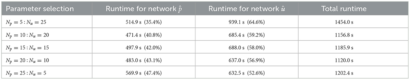
Table 1. Runtime overheads of five different parameter selections for FS-PINNs architecture of Example 1.

Figure 3 tracks the trends of all MSE terms during different parameter selections training procedures, revealing that the case N_p = 25:N_u = 5 performs worst, and the case N_p = 5:N_u = 25 is less stable. The inadequate representation ability of tiny networks leads to inaccurate solutions. Network approximations $\widehat{p}$ and $\widehat{u}$ depend on the interdependent loss functions for FS-PINNs. On the other hand, the trends of the remaining three cases are quite similar, which implies that FS-PINNs with reasonable architecture can withstand accuracy issues.

FIGURE 3

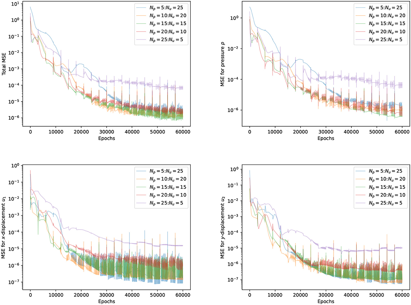
Figure 3. Trends of all the MSE terms at T = 0.5 for five different FS-PINNs architecture during training with respect to epoch.

4.2.2. Acceleration effect of the FS-PINNs training

This section demonstrates the acceleration effect of the FS-PINNs over the classical PINNs. Biot's equations are solved using both methods with the same setup as in Example 1. The number of neurons for the two networks in FS-PINNs is fixed to N_p = N_u = 15 (as indicated by Table 1), while the total number of neurons in classical PINNs is set to N_n = 30 with the number of layers L_n = 3. To examine the effect of the number of epochs optimizing networks and the number of fixed-stress iterations, we then conduct the test with a constant number of the multiplication of the above two number, which is set to 20, 000.

Figure 4 shows the trends of MSE terms for solving the problem in Example 1. We present the results generated by one classical PINN and four FS-PINNs under identical conditions, which demonstrates the acceleration effect of FS-PINNs. By decoupling the original optimization problem into two small sub-problems, together with the fixed-stress coefficient L < 1, FS-PINNs increase efficiency and maintain certain accuracy. From this perspective, FS-PINNs offer more flexibility in solving the problem through different setting of optimizing epoch and fixed-stress iteration. In Figure 4, we can see that a smaller number of epochs lead to faster convergence initially but lower accuracy eventually. Since the fixed-stress splitting method is a numerical approach, high accuracy is not essential for each fixed-stress step. It implies that a large number of optimizing epochs is not so helpful.

FIGURE 4

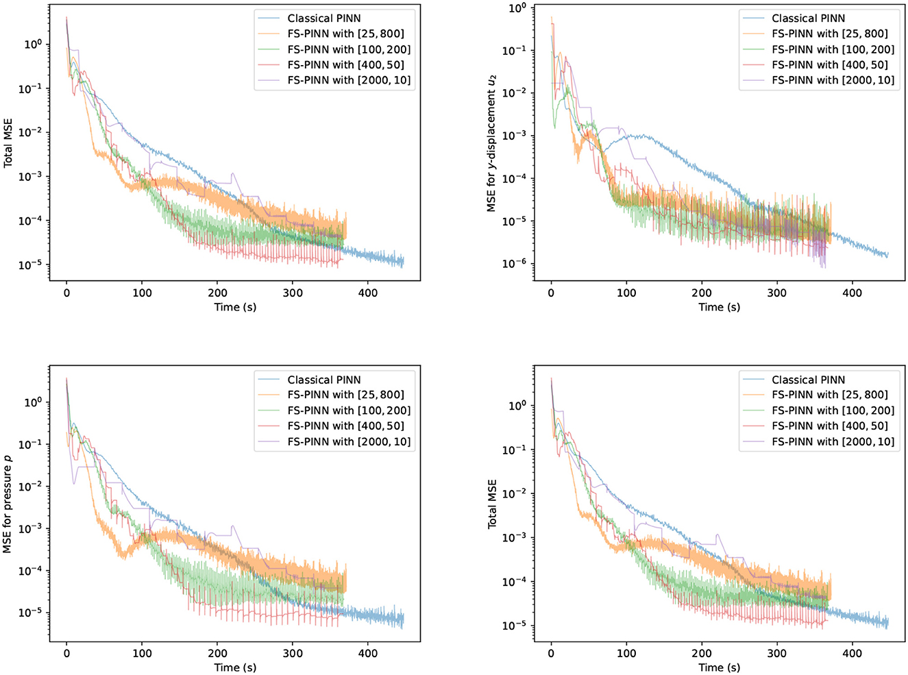
Figure 4. Trends of all the MSE terms at T = 0.5 for one classical PINN and four FS-PINNs with [the number of epochs training networks, the number of fixed-stress iterations] during training with respect to runtime overhead.

Among all the results generated by FS-PINNs, here we consider in-depth observations for the case of [400, 50]. Here, 400 means the number of epochs, and 50 means the number of fixed-stress iterations. To test the cases with a larger parameter λ, we also include the testing result when the Poisson ratio ν = 0.49 for Example 1. Figure 5 provides a comparison between the analytical solution and the numerical solution given by FS-PINNs with [400, 50]. Theses results show that the proposed FS-PINNs with ν = 0.3 and ν = 0.49 accurately predict the pressure p and displacement u with errors within an acceptable tolerance range. However, it is true that when λ is large, to obtain a more accurate solution, we need to put a relatively large weight for the first equation in the total loss function. And also, we need to increase the number of epochs and set a finer learning rate for the training of the network for u.

FIGURE 5

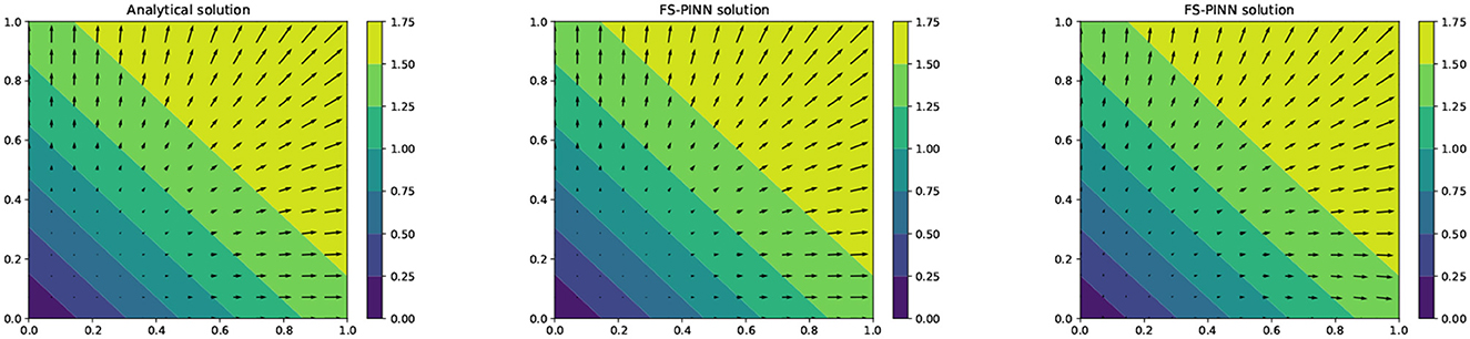
Figure 5. A comparison of the analytical solution (left), the FS-PINN solution with ν = 0.3 (middle), and the FS-PINN solution ν = 0.49 (right) at T = 0.5 for Example 1.

4.3. Example 2

The Biot's problem with mixed boundary conditions presented in [2] is tested. We consider the square domain Ω = [0, 1]², with Dirichlet boundary Γ₁∪Γ₃ and Neumann boundary Γ₂∪Γ₄. Specifically, Γ₁ = (1, y);0 ≤ y ≤ 1, Γ₂ = (x, 0);0 ≤ x ≤ 1, Γ₃ = (0, y);0 ≤ y ≤ 1, and Γ₄ = (x, 1);0 ≤ x ≤ 1. Setting the final time to T = 0.2, we choose the body force g, the source or sink term f, as well as the initial and boundary conditions such that exact solutions are as follows.

$\begin{array}{l}{u}_1=e^{-t}\left(sin(2\pi y)(cos(2\pi x)-1)+\frac{1}{\mu +\text{λ}}sin(\pi x)sin(\pi y)\right),\\ u_2=e^{-t}\left(sin(2\pi x)(1-cos(2\pi y))+\frac{1}{\mu +\text{λ}}sin(\pi x)sin(\pi y)\right),\\ p=e^{-t}sin(\pi x)sin(\pi y).\end{array}$

The parameters of the model are E = 1.0, ν = 0.3, α = 1.0, M = 1.0, K = 1.

In dealing with mixed boundary conditions, it is necessary to select suitable loss functions capable of handling both Dirichlet and Neumann boundary conditions. To this end, we follow the approach taken in [28, 32] and employ the corresponding loss functions ${\mathcal{L}}_p$ and ${\mathcal{L}}_u$ for pressure and displacement, respectively. In this test, following the result in Section 4.2.2., we employ the FS-PINN with [400, 50] using the same architecture to solve Example 2.

In Figure 6, we compare the analytical solution with our FS-PINN solution and observe that our approach can approximate solutions for problems with mixed boundary conditions. However, its performance is not as good as that of solving the pure Dirichlet problem in Example 1. The network approximations in the boundary region are sub-optimal because all the parameters used were selected to solve Example 1. Hence, the complexity of Example 2 presents a challenge to our network, which could potentially be overcome by optimizing the parameters, such as by using additional collocation points in the boundary region.

FIGURE 6

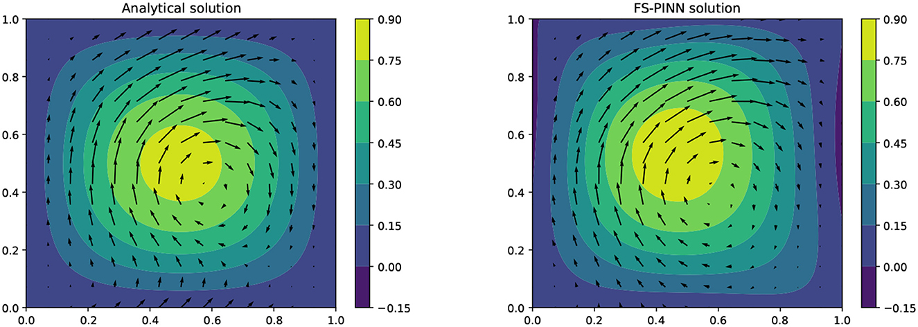
Figure 6. A comparison of the analytical solution (left) and the FS-PINN solution with [400, 50] (right) at T = 0.2 for Example 2.

4.4. Example 3

The Barry-Mercer's problem is a classical benchmark problem of porous media involving injection of fluids [14, 31, 35, 36]. It is a two-dimensional problem in the square domain Ω = [0, 1]² that has a point source f located at (x₀, y₀) = (0.25, 0.25), which makes it challenging to solve numerically. Figure 7 depicts the boundary conditions under consideration.

FIGURE 7

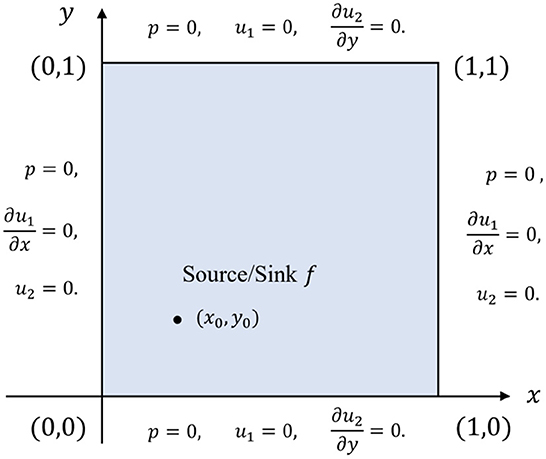
Figure 7. Boundary conditions for the Barry-Mercer's problem.

As for the initial conditions, we set

$\begin{array}{ll}u=0,p=0\text{in Ω}\times \left\{0\right\}.& (55)\end{array}$

To define the body force term g and the source/sink term f, we use the following expressions:

$\begin{array}{ll}g=0,f=2\delta (x-x_0)\delta (y-y_0)sin(t),& (56)\end{array}$

where δ denotes the Dirac function. We approximate the Dirac function using the Gaussian distribution [31], that is, $\delta (x)\approx \frac{1}{c_g\sqrt{\pi }}{e}^{-{(x/c_g)}^2}$ with c_g = 0.04. The physical parameters are specified as follows:

$\begin{array}{ll}1/M=0,\alpha =1.0,\text{\hspace{1em}λ}=0.2,\mu =0.4,K=1.0.& (57)\end{array}$

Denote λ_n = nπ, λ_q = qπ, and ${\text{λ}}_{nq}={\text{λ}}_n^2+{\text{λ}}_q^2$, then the analytical solution is as follows:

$\begin{array}{l}p(x,y,t)=-4{\displaystyle \sum _{n=1}^{\infty }}{\displaystyle \sum _{q=1}^{\infty }}\widehat{p}(n,q,t)sin({\text{λ}}_{n}x)sin({\text{λ}}_{q}y),\\ u_1(x,y,t)=4{\displaystyle \sum _{n=1}^{\infty }}{\displaystyle \sum _{q=1}^{\infty }}{û}_1(n,q,t)cos({\text{λ}}_{n}x)sin({\text{λ}}_{q}y),\\ u_2(x,y,t)=4{\displaystyle \sum _{n=1}^{\infty }}{\displaystyle \sum _{q=1}^{\infty }}{û}_2(n,q,t)sin({\text{λ}}_{n}x)cos({\text{λ}}_{q}y),\end{array}$

where

$\begin{array}{l}\widehat{p}(n,q,t)=-\frac{2sin({\text{λ}}_n{x}_0)sin({\text{λ}}_q{y}_0)}{{\text{λ}}_{nq}^2+1}({\text{λ}}_{nq}sint-cost+e^{-{\text{λ}}_{nq}t}),\\ {û}_1(n,q,t)=\frac{{\text{λ}}_n}{{\text{λ}}_{nq}}\widehat{p}(n,q,t),{û}_2(n,q,t)=\frac{{\text{λ}}_q}{{\text{λ}}_{nq}}\widehat{p}(n,q,t).\end{array}$

In this case, we use the same architecture as in Section 4.2.2, which is the FS-PINN with [400, 50], to solve Barry-Mercer's problem. As mentioned in the literature [37], networks training relies on the propagation of information from initial and boundary points to the interior points. To improve the performance of our FS-PINN, we apply weighted loss functions proposed in [32], and increase the weights of the initial and boundary loss terms. Specifically, we replace $\frac{1}{N_3}$, $\frac{1}{N_5}$ with $\frac{1000}{N_3}$, $\frac{100}{N_5}$ in the loss functions (27), (28), respectively. The solution obtained from our FS-PINN closely matches the analytic solution at T = π/4 for Example 3, as demonstrated in Figure 8. This indicates the effectiveness of our approach in approximating the analytic solution.

FIGURE 8

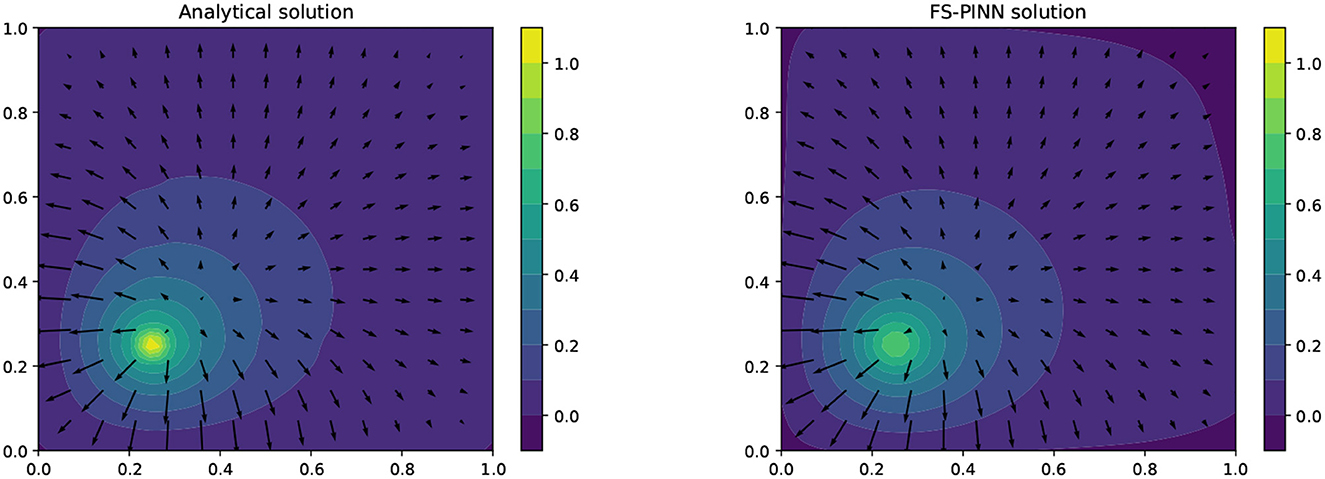
Figure 8. A comparison of the analytical solution (left) and the FS-PINN solution (right) at T = π/4 for Example 3.

5. Conclusion

This paper presents a new approach to solving Biot's consolidation model by combining Physics-informed neural networks (PINNs) with the fixed-stress splitting method. We demonstrate that our method achieves faster convergence and lower computational costs than the neural network methods which solve Biot's problem in a monolithic way. We provide a theoretical analysis to show the convergence of our proposed FS-PINNs. The numerical experiments illustrate the effectiveness of our approach on various test cases with different boundary conditions and physical parameters.

While our approach has several advantages over some traditional methods for solving poroelastic models, such as being meshless, not requiring inf-sup stability, there are also some limitations and challenges that need to be addressed in future work. These include choosing optimal network architectures and parameters for different problems, improving accuracy and reducing computational costs even further, and extending the approach to other PDE problems and multi-physics problems. We hope that our work can inspire more research on combining deep learning techniques with iterative methods for solving PDEs.

Data availability statement

The original contributions presented in the study are included in the article/supplementary material, further inquiries can be directed to the corresponding author.

Author contributions

MC: conceptualization, investigation, writing—original draft, validation, methodology, writing—review and editing, supervision, formal analysis, and funding acquisition. HG: investigation, writing—original draft, validation, visualization, writing—review and editing, formal analysis, and data curation. PH: investigation, writing—original draft, validation, visualization, writing—review and editing, software, and data curation. JL: conceptualization, investigation, funding acquisition, validation, methodology, project administration, and supervision. All authors contributed to the article and approved the submitted version.

Funding

The work of MC was partially supported by the NIH-RCMI grant through 347 U54MD013376, the affiliated project award from the Center for Equitable Artificial Intelligence and Machine Learning Systems (CEAMLS) at Morgan State University (project ID 02232301), and the National Science Foundation awards (1831950 and 2228010). The work of HG, PH, and JL were partially supported by the NSF of China No. 11971221, Guangdong NSF Major Fund No. 2021ZDZX1001, the Shenzhen Sci-Tech Fund Nos. RCJC20200714114556020, JCYJ20200109115422828, and JCYJ20190809150413261, National Center for Applied Mathematics Shenzhen, and SUSTech International Center for Mathematics.

Conflict of interest

The authors declare that the research was conducted in the absence of any commercial or financial relationships that could be construed as a potential conflict of interest.

Publisher's note

All claims expressed in this article are solely those of the authors and do not necessarily represent those of their affiliated organizations, or those of the publisher, the editors and the reviewers. Any product that may be evaluated in this article, or claim that may be made by its manufacturer, is not guaranteed or endorsed by the publisher.

References

1. Biot MA. General theory of three-dimensional consolidation. J Appl Phys. (1941) 12:155–64. doi: 10.1063/1.1712886

CrossRef Full Text | Google Scholar

2. Ju G, Cai M, Li J, Tian J. Parameter-robust multiphysics algorithms for Biot model with application in brain edema simulation. Math Comput Simul. (2020) 177:385–403. doi: 10.1016/j.matcom.2020.04.027

PubMed Abstract | CrossRef Full Text | Google Scholar

3. Kim J, Tchelepi HA, Juanes R. Stability and convergence of sequential methods for coupled flow and geomechanics: fixed-stress and fixed-strain splits. Comput Methods Appl Mech Eng. (2011) 200:1591–606. doi: 10.1016/j.cma.2010.12.022

CrossRef Full Text | Google Scholar

4. Ženíšek A. The existence and uniqueness theorem in Biot's consolidation theory. Aplik Matem. (1984) 29:194–211. doi: 10.21136/AM.1984.104085

CrossRef Full Text | Google Scholar

5. Showalter RE. Diffusion in poro-elastic media. J Math Anal Appl. (2000) 251:310–40. doi: 10.1006/jmaa.2000.7048

PubMed Abstract | CrossRef Full Text | Google Scholar

6. Phillips PJ, Wheeler MF. A coupling of mixed and continuous Galerkin finite element methods for poroelasticity I: the continuous in time case. Comput Geosci. (2007) 11:131–44. doi: 10.1007/s10596-007-9045-y

CrossRef Full Text | Google Scholar

7. Nordbotten JM. Stable cell-centered finite volume discretization for Biot equations. SIAM J Numer Anal. (2016) 54:942–68. doi: 10.1137/15M1014280

CrossRef Full Text | Google Scholar

8. Coulet J, Faille I, Girault V, Guy N, Nataf F. A fully coupled scheme using virtual element method and finite volume for poroelasticity. Comput Geosci. (2020) 24:381–403. doi: 10.1007/s10596-019-09831-w

CrossRef Full Text | Google Scholar

9. Yi SY. A coupling of nonconforming and mixed finite element methods for Biot's consolidation model. Numer Methods Part Diff Equat. (2013) 29:1749–77. doi: 10.1002/num.21775

CrossRef Full Text | Google Scholar

10. Yi SY. A study of two modes of locking in poroelasticity. SIAM J Numer Anal. (2017) 55:1915–36. doi: 10.1137/16M1056109

CrossRef Full Text | Google Scholar

11. Rodrigo C, Gaspar F, Hu X, Zikatanov L. Stability and monotonicity for some discretizations of the Biot's consolidation model. Comput Methods Appl Mech Eng. (2016) 298:183–204. doi: 10.1016/j.cma.2015.09.019

CrossRef Full Text | Google Scholar

12. Lee JJ, Mardal KA, Winther R. Parameter-robust discretization and preconditioning of Biot's consolidation model. SIAM J Sci Comput. (2017) 39:A1–24. doi: 10.1137/15M1029473

CrossRef Full Text | Google Scholar

13. Cai M, Zhang G. Comparisons of some iterative algorithms for Biot equations. Int J Evol Equat. (2017) 10:267–82.

PubMed Abstract | Google Scholar

14. Phillips PJ, Wheeler MF. Overcoming the problem of locking in linear elasticity and poroelasticity: an heuristic approach. Comput Geosci. (2009) 13:5–12. doi: 10.1007/s10596-008-9114-x

CrossRef Full Text | Google Scholar

15. Rodrigo C, Hu X, Ohm P, Adler JH, Gaspar FJ, Zikatanov L. New stabilized discretizations for poroelasticity and the Stoke's equations. Comput Methods Appl Mech Eng. (2018) 341:467–84. doi: 10.1016/j.cma.2018.07.003

CrossRef Full Text | Google Scholar

16. Feng X, Ge Z, Li Y. Analysis of a multiphysics finite element method for a poroelasticity model. IMA J Numer Anal. (2018) 38:330–59. doi: 10.1093/imanum/drx003

CrossRef Full Text | Google Scholar

17. Oyarzúa R, Ruiz-Baier R. Locking-free finite element methods for poroelasticity. SIAM Journal on Numerical Anal. (2016) 54:2951–73. doi: 10.1137/15M1050082

CrossRef Full Text | Google Scholar

18. Yi SY, Bean ML. Iteratively coupled solution strategies for a four-field mixed finite element method for poroelasticity. Int J Numer Analyt Methods Geomech. (2017) 41:159–79. doi: 10.1002/nag.2538

CrossRef Full Text | Google Scholar

19. Mikelić A, Wheeler MF. Convergence of iterative coupling for coupled flow and geomechanics. Comput Geosci. (2013) 17:455–61. doi: 10.1007/s10596-012-9318-y

CrossRef Full Text | Google Scholar

20. Mikelić A, Wang B, Wheeler MF. Numerical convergence study of iterative coupling for coupled flow and geomechanics. Comput Geosci. (2014) 18:325–41. doi: 10.1007/s10596-013-9393-8

CrossRef Full Text | Google Scholar

21. Both JW, Borregales M, Nordbotten JM, Kumar K, Radu FA. Robust fixed stress splitting for Biot's equations in heterogeneous media. Appl Math Lett. (2017) 68:101–8. doi: 10.1016/j.aml.2016.12.019

CrossRef Full Text | Google Scholar

22. Bause M, Radu FA, Köcher U. Space-time finite element approximation of the Biot poroelasticity system with iterative coupling. Comput Methods Appl Mech Eng. (2017) 320:745–68. doi: 10.1016/j.cma.2017.03.017

CrossRef Full Text | Google Scholar

23. Storvik E, Both JW, Kumar K, Nordbotten JM, Radu FA. On the optimization of the fixed-stress splitting for Biot's equations. Int J Numer Methods Eng. (2019) 120:179–94. doi: 10.1002/nme.6130

CrossRef Full Text | Google Scholar

24. Borregales M, Kumar K, Radu FA, Rodrigo C, Gaspar FJ. A partially parallel-in-time fixed-stress splitting method for Biot's consolidation model. Comput Math Appl. (2019) 77:1466–78. doi: 10.1016/j.camwa.2018.09.005

CrossRef Full Text | Google Scholar

25. Raissi M, Perdikaris P, Karniadakis GE. Physics-informed neural networks: a deep learning framework for solving forward and inverse problems involving nonlinear partial differential equations. J Comput Phys. (2019) 378:686–707. doi: 10.1016/j.jcp.2018.10.045

CrossRef Full Text | Google Scholar

26. Lu L, Meng X, Mao Z, Karniadakis GE. DeepXDE: a deep learning library for solving differential equations. SIAM Rev. (2021) 63:208–28. doi: 10.1137/19M1274067

CrossRef Full Text | Google Scholar

27. Amini D, Haghighat E, Juanes R. Inverse modeling of nonisothermal multiphase poromechanics using physics-informed neural networks. arXiv preprint arXiv:220903276. (2022). doi: 10.1016/j.jcp.2023.112323

CrossRef Full Text | Google Scholar

28. Kadeethum T, Jørgensen TM, Nick HM. Physics-informed neural networks for solving nonlinear diffusivity and Biot's equations. PLoS ONE. (2020) 15:e0232683. doi: 10.1371/journal.pone.0232683

PubMed Abstract | CrossRef Full Text | Google Scholar

29. Millevoi C, Spiezia N, Ferronato M. On Physics-Informed Neural Networks Architecture for Coupled Hydro-Poromechanical Problems. (2022). doi: 10.2139/ssrn.4074416

CrossRef Full Text | Google Scholar

30. Bekele YW. Physics-informed deep learning for flow and deformation in poroelastic media. arXiv preprint arXiv:201015426. (2020).

Google Scholar

31. Haghighat E, Amini D, Juanes R. Physics-informed neural network simulation of multiphase poroelasticity using stress-split sequential training. Comput Methods Appl Mech Eng. (2022) 397:115141. doi: 10.1016/j.cma.2022.115141

CrossRef Full Text | Google Scholar

32. Amini D, Haghighat E, Juanes R. Physics-informed neural network solution of thermo-hydro-mechanical (THM) processes in porous media. arXiv preprint arXiv:220301514. (2022). doi: 10.1061/(ASCE)EM.1943-7889.0002156

PubMed Abstract | CrossRef Full Text | Google Scholar

33. De Ryck T, Jagtap AD, Mishra S. Error estimates for physics informed neural networks approximating the Navier-Stokes equations. arXiv preprint arXiv:220309346. (2022). doi: 10.1093/imanum/drac085

CrossRef Full Text | Google Scholar

34. Paszke A, Gross S, Massa F, Lerer A, Bradbury J, Chanan G, et al. PyTorch: An imperative style, high-performance deep learning library. In:Wallach H, Larochelle H, Beygelzimer A, Alche-Buc F, Fox E, Garnett R, , editors. Advances in Neural Information Processing Systems, Vol. 32. Curran Associates (2019). Available online at: https://proceedings.neurips.cc/paper_files/paper/2019/file/bdbca288fee7f92f2bfa9f7012727740-Paper.pdf

Google Scholar

35. Barry S, Mercer G. Exact solutions for two-dimensional time-dependent flow and deformation within a poroelastic medium. J Appl Mech. (1999) 66:536–40. doi: 10.1115/1.2791080

CrossRef Full Text | Google Scholar

36. Phillips PJ. Finite Element Methods in Linear Poroelasticity: Theoretical and Computational Results. Austin, TX: The University of Texas at Austin (2005).

PubMed Abstract | Google Scholar

37. Daw A, Bu J, Wang S, Perdikaris P, Karpatne A. Mitigating propagation failures in pinns using evolutionary sampling, conference paper at ICLR 2023?. (Under review).

Google Scholar

Appendix

Proof of Theorem 2.1

Proof. Subtracting (6), (9) from (1), (2), respectively, we shall derive

$\begin{array}{ll}\left(\frac{1}{M}+{\beta }_{FS}\right){\partial }_t{e}_p^{n+1}-\nabla ·K\nabla e_p^{n+1}=-\alpha \nabla ·{\partial }_t{e}_u^n+{\beta }_{FS}{\partial }_t{e}_p^n,& (58)\end{array}$

$\begin{array}{ll}-\nabla ·\sigma (e_u^{n+1})+\alpha \nabla e_p^{n+1}=0.& (59)\end{array}$

After differentiating (2) with respect to t, one has

$\begin{array}{ll}-\nabla ·\sigma ({\partial }_t{e}_u^{n+1})+\alpha \nabla {\partial }_t{e}_p^{n+1}=0.& (60)\end{array}$

We multiply (1), (3) by ${\partial }_t{e}_p^{n+1}$, ${\partial }_t{e}_u^n$, respectively, and use integration by parts to obtain

$\begin{array}{l}\left(\frac{1}{M}+{\beta }_{FS}\right){\displaystyle {\int }_0^T{\displaystyle {\int }_{\text{Ω}}{({\partial }_t{e}_p^{n+1})}^2}}dxdt+\\ \frac{K}{2}{\displaystyle {\int }_{\text{Ω}}{(\nabla e_p^{n+1}(T))}^2}dx\\ =-\alpha {\displaystyle {\int }_0^T{\displaystyle {\int }_{\text{Ω}}(\nabla ·{\partial }_t{e}_u^n)({\partial }_t{e}_p^{n+1})}}dxdt+\\ {\beta }_{FS}{\displaystyle {\int }_0^T{\displaystyle {\int }_{\text{Ω}}({\partial }_t{e}_p^n)({\partial }_t{e}_p^{n+1})}}dxdt,& (61)\end{array}$

$\begin{array}{l}2\mu {\displaystyle {\int }_0^T{\displaystyle {\int }_{\text{Ω}}\epsilon }}({\partial }_t{e}_u^{n+1}):\epsilon ({\partial }_t{e}_u^n)dxdt+\\ \text{λ}{\displaystyle {\int }_0^T{\displaystyle {\int }_{\text{Ω}}(\nabla ·{\partial }_t{e}_u^{n+1})(\nabla ·{\partial }_t{e}_u^n)}}dxdt\\ =\alpha {\displaystyle {\int }_0^T{\displaystyle {\int }_{\text{Ω}}(\nabla ·{\partial }_t{e}_u^n)({\partial }_t{e}_p^{n+1})}}dxdt.& (62)\end{array}$

Combining Equations (4) and (5) results in the following equation.

$\begin{array}{l}\frac{1}{M}{\displaystyle {\int }_0^T{\displaystyle {\int }_{\text{Ω}}{({\partial }_t{e}_p^{n+1})}^2}}dxdt+\frac{K}{2}{\displaystyle {\int }_{\text{Ω}}{(\nabla e_p^{n+1}(T))}^2}dx+\\ 2\mu {\displaystyle {\int }_0^T{\displaystyle {\int }_{\text{Ω}}\epsilon }}({\partial }_t{e}_u^{n+1}):\epsilon ({\partial }_t{e}_u^n)dxdt\\ +\text{ λ}{\displaystyle {\int }_0^T{\displaystyle {\int }_{\text{Ω}}(\nabla ·{\partial }_t{e}_u^{n+1})(\nabla ·{\partial }_t{e}_u^n)}}dxdt\\ {\beta }_{FS}{\displaystyle {\int }_0^T{\displaystyle {\int }_{\text{Ω}}({\partial }_t{e}_p^{n+1})({\partial }_t{e}_p^{n+1}-{\partial }_t{e}_p^n)}}dxdt=0.& (63)\end{array}$

Applying the algebraic identities (46) to (6), we derive

$\begin{array}{l}\left(\frac{1}{M}+\frac{{\beta }_{FS}}{2}\right){\displaystyle {\int }_0^T{\displaystyle {\int }_{\text{Ω}}{({\partial }_t{e}_p^{n+1})}^2}}dxdt+\frac{K}{2}{\displaystyle {\int }_{\text{Ω}}{(\nabla e_p^{n+1}(T))}^2}dx\\ +\frac{\mu }{2}{\displaystyle {\int }_0^T{\displaystyle {\int }_{\text{Ω}}\epsilon }}({\partial }_t{e}_u^{n+1}+{\partial }_t{e}_u^n):\epsilon ({\partial }_t{e}_u^{n+1}+{\partial }_t{e}_u^n)dxdt\\ +\frac{\text{λ}}{4}{\displaystyle {\int }_0^T{\displaystyle {\int }_{\text{Ω}}{\left(\nabla ·({\partial }_t{e}_u^{n+1}+{\partial }_t{e}_u^n)\right)}^2}}dxdt++\\ \frac{{\beta }_{FS}}{2}{\displaystyle {\int }_0^T{\displaystyle {\int }_{\text{Ω}}{({\partial }_t{e}_p^{n+1}-{\partial }_t{e}_p^n)}^2}}dxdt\\ =\frac{\mu }{2}{\displaystyle {\int }_0^T{\displaystyle {\int }_{\text{Ω}}\epsilon }}({\partial }_t{e}_u^{n+1}-{\partial }_t{e}_u^n):\epsilon ({\partial }_t{e}_u^{n+1}-{\partial }_t{e}_u^n)dxdt\\ +\frac{\text{λ}}{4}{\displaystyle {\int }_0^T{\displaystyle {\int }_{\text{Ω}}{\left(\nabla ·({\partial }_t{e}_u^{n+1}-{\partial }_t{e}_u^n)\right)}^2}}dxdt+\\ \frac{{\beta }_{FS}}{2}{\displaystyle {\int }_0^T{\displaystyle {\int }_{\text{Ω}}{({\partial }_t{e}_p^n)}^2}}dxdt.& (64)\end{array}$

The difference of two successive iterations based on (2) will yield

$\begin{array}{ll}-\nabla ·\sigma ({\partial }_t{e}_u^{n+1}-{\partial }_t{e}_u^n)+\alpha \nabla ({\partial }_t{e}_p^{n+1}-{\partial }_t{e}_p^n)=0.& (65)\end{array}$

Multiplying (8) by $({\partial }_t{e}_u^{n+1}-{\partial }_t{e}_u^n)$, integration by parts, and then applying Cauchy-Schwarz inequality, we derive that

$\begin{array}{l}2\mu {\displaystyle {\int }_0^T{\displaystyle {\int }_{\text{Ω}}\epsilon }}({\partial }_t{e}_u^{n+1}-{\partial }_t{e}_u^n):\epsilon ({\partial }_t{e}_u^{n+1}-{\partial }_t{e}_u^n)dxdt\\ +\text{ λ}{\displaystyle {\int }_0^T{\displaystyle {\int }_{\text{Ω}}{\left(\nabla ·({\partial }_t{e}_u^{n+1}-{\partial }_t{e}_u^n)\right)}^2}}dxdt+\\ \le \frac{{\alpha }^2}{\frac{2\mu }{d}+\text{λ}}{\displaystyle {\int }_0^T{\displaystyle {\int }_{\text{Ω}}{({\partial }_t{e}_p^{n+1}-{\partial }_t{e}_p^n)}^2}}dxdt.& (66)\end{array}$

Discarding the second, third, and fourth terms in (7), we choose ${\beta }_{FS}\ge \frac{{\alpha }^2}{2\left(\frac{2\mu }{d}+\text{λ}\right)}$ to obtain

$\begin{array}{ll}{\displaystyle {\int }_0^T{\displaystyle {\int }_{\text{Ω}}{({\partial }_t{e}_p^{n+1})}^2}}dxdt\le \frac{{\beta }_{FS}}{{\beta }_{FS}+\frac{2}{M}}{\displaystyle {\int }_0^T{\displaystyle {\int }_{\text{Ω}}{({\partial }_t{e}_p^n)}^2}}dxdt,& (67)\end{array}$

which directly implies (14).