Lp-Sampling recovery for non-compact subclasses of L∞

1. Introduction

In this article, we continue to study the approximation power of Smolyak sparse grid sampling recovery for multivariate function classes with small mixed smoothness $S_{p,\theta }^{r}B({\left[0,1\right]}^d)$ and $S_{p,\theta }^{r}F({\left[0,1\right]}^d)$ based on the multivariate Faber representation [1, 2] of f. The advantage of such a representation is the fact that the coefficient functionals only use discrete functional values of f, see (2.1) and (2.3) below, which allow for various applications. For instance, Kempka et al. [3] used the Faber system to analyze the path regularity of the Brownian motion, where a small smoothness setting is also required.

It provides a powerful tool for studying various situations of the sampling recovery problem where errors are measured in L_q. Surprisingly, the proposed method turned out to be sharp in several regimes. A systematic discretization of multivariate functions with mixed smoothness in terms of Faber coefficients is given [1, 2, 4, 5], see also [6] for further history. In this article, we study an endpoint situation for the sampling recovery problem on the cube [0, 1]^d, where r = 1/p in the source space and the fine parameter θ ≤ 1 is sufficiently small. This still allows for an embedding into the continuous functions (therefore making function evaluations possible). However, the embedding into L_q is only compact if q < ∞.

Recent observations regarding the problem of optimal sampling recovery of function classes in L₂ bring classes with mixed smoothness to the focus again since several newly developed techniques only work for Hilbert-Schmidt operators [7–9] or, more generally, in situations where certain asymptotic characteristics (approximation numbers) are square summable [10, 11]. We need new techniques for situations where this is not the case. In Temlyakov and Ullrich [12, 13], the authors consider the range of small smoothness where one is far away from square summability of the corresponding widths. However, we have the compact embedding into L_∞ for those examples. This embedding seems to be of crucial importance when (non-linear) sampling widths (_ϱm)m, defined by

${\varrho }_m(\text{F},X):={\displaystyle \underset{x^1,...,x^m}{inf}}{\displaystyle \underset{R:{ℂ}^m\to X}{inf}}{\displaystyle \underset{f\in \text{F}}{sup}}||f-R(f(x^1),...,f(x^m))|X||,$

with X = L₂ are related to certain asymptotic characteristics such as Kolmogorov (_dm)m or best m-term trigonometric widths (_σm)m in L_∞. It has been shown by Temlyakov [14], Bartel et al. [9] and Jahn et al. [15] that the following inequalities hold for relevant function classes F

$\begin{array}{ll}{\varrho }_{bm}^{lin}(F,L_2)\le \frac{C}{{(b-1)}^{3/2}}{d}_m(F,L_{\infty }),& (1.1)\end{array}$

$\begin{array}{l}{\varrho }_{\lceil Dm{(\log m)}^3\rceil }(F,L_2)\lesssim {\sigma }_m(F,L_{\infty }),\end{array}$

Here, we have some constants C, D > 0 and oversampling parameter 1 < b ≤ 2 in the first relation. We speak about linear sampling widths denoted by ${({\varrho }_m^{\text{lin}})}_m$ if the reconstruction mapping R is linear. The second relation might not need a compact embedding into L_∞ at first glance. However, the proof heavily relies on certain compactness properties of the embedding, see [15]. Clearly, a compact embedding into L_∞ allows us to use the decaying Kolmogorov widths for controlling the linear sampling widths. As discussed by Temlyakov and Ullrich [12], sparse grid techniques [16] perform asymptotically worse by a log factor for classes with mixed smoothness compactly embedded into L_∞.

In this article, we continue our research in this direction. Note that there are several relevant (multivariate) function classes F which are continuously but not compactly embedded into L_∞. Thus, at least the first relation in (1.1) is useless. In fact, only few results have been published on reconstructing functions from samples, which only satisfy a Besov regularity with smoothness r = 1/p or Sobolev type regularity with r = 1 and p = 1. Our aim is to investigate this problem systematically in the Fourier analytic context. As a first step, we prove the following relation for the Faber coefficients $d_{j,k}^2(f)$ of f, namely

$\begin{array}{l}\underset{j\in {\mathbb{N}}_{-1}^d}{\sup }{\left({\displaystyle \sum _{k\in \mathbb{Z}d}|d_{j,k}^2(f){|}^p}\right)}^{1/p}\lesssim \text{ |}|f|S_{p,\min \{p,1\}}^{1/p}B({ℝ}^d)||\end{array}$

in case 1/2 ≤ p ≤ ∞. Our contribution is a proof that works for Fourier analytic defined spaces and allows for incorporating also the extreme cases $S_{1/2,1/2}^{2}B({ℝ}^d)$ and $S_{\infty ,1}^{0}B({ℝ}^d)$ [in contrast to Dũng [17], Theorem 3.2]. It represents an extreme case of the considered limit situation, in which the Faber approximation can benefit from the highest regularity of smoothness equals 2. The above relation directly implies that the truncated Faber representation still works well when we consider errors in L_q with q < ∞. We make progress toward the solution of an open problem mentioned [[18], Section 3.2]. The univariate class $B_{p,1}^{1/p}\left(\right[0,1\left]\right)$ and its approximation by equidistant samples in [0, 1] have been considered by Oswald [19] in the beginning of the 80s. In 2011, Dũng [[17], Theorem 3.2] obtained results for the multivariate situation in the framework of Besov spaces with a bounded mixed difference. In contrast to the spaces considered by Dũng [17], we highlight that the Besov and Triebel-Lizorkin spaces considered here are defined using Fourier analytic building blocks. Note that in the considered limiting situation and p < 1, it is not yet known whether these spaces coincide with the ones considered by Dũng [see [20], Remark 2.3.4/2].

Notation. In general, ℕ denotes the natural numbers, ℕ₀ = ℕ ∪ {0}, ℕ ₋₁ = ℕ₀ ∪ {−1}, ℤ denotes the integers, ℝ denotes the real numbers, and ℂ denotes the complex numbers. The letter d is always reserved for the underlying dimension in ℝ^d, ℤ^d, etc. For a ∈ ℝ, we denote a₊: = max{a, 0}. For 0 < p ≤ ∞ and x ∈ ℝ^d, we denote $|x{|}_p={(\sum _{i=1}^d|x_i{|}^p)}^{1/p}$ with the usual modification in the case p = ∞. We further denote x₊ : = ((_x1)+, …, (_xd)+) and |x|₊ : = |x₊|₁. By (x₁, …, x_d) > 0, we mean that each coordinate is positive. If X and Y are two (quasi-)normed spaces, the (quasi-)norm of an element x in X will be denoted by ||x|X||. The symbol X↪Y indicates that the identity operator is continuous. For two sequences a_n and b_n, we will write a_n ≲ b_n if there exists a constant c > 0 such that a_n ≤ cb_n for all n. We will write a_n ≍ b_n if a_n ≲ b_n and b_n ≲ a_n.

2. The tensor Faber basis

As a main tool, we will use decompositions of functions in terms of a Faber series expansion.

2.1. The univariate Faber basis

Let us briefly recall the basic facts about the Faber basis taken from [[4], 3.2.1 and 3.2.2]. For j ∈ ℕ₀ and $k\in {𝔻}_j:=\left\{0,1,...,2^j-1\right\}$, we denote the dyadic interval by I_j,k given by

$I_{j,k}=\left[2^{-j}k,2^{-j}(k+1)\right].$

Definition 2.1. [The univariate Faber system] Let

$\begin{array}{l}h(t)=\{\begin{array}{l}1\text{ : }t\in [0,1/2),\\ -1\text{ : }t\in (1/2,1],and\\ 0\text{ : otherwise},\end{array}\end{array}$

the Haar function and v(x) be the integrated Haar function, i.e.,

$\begin{array}{l}\begin{array}{l}v(x):=2{\displaystyle {\int }_0^{x}h(t)dt,}x\in ℝ,\hfill \end{array}\end{array}$

and for j ∈ ℕ₀ and k ∈ 𝔻_j, then

$\begin{array}{l}{v}_{j,k}(·)=v(2^j·-k).\end{array}$

For notational reasons, we let v_−1,0 = x and v_−1,1 : = 1 − x for j = −1 and obtain the univariate Faber basis

$\left\{v_{j,k}:j\in {\mathbb{N}}_{-1},k\in {\text{𝔻}}_j\right\},$

where 𝔻₋₁: = 𝔻₁ = {0, 1}.

Faber [21] observed that every continuous (non-periodic) function f on [0, 1] can be represented as

$\begin{array}{ll}f(x)=f(0)·(1-x)+f(1)·x-\frac{1}{2}{\displaystyle \sum _{j=0}^{\infty }}{\displaystyle \sum _{k=0}^{2^j-1}}{\text{Δ}}_{2^{-j-1}}^2(f,2^{-j}k)v_{j,k}(x),& (2.1)\end{array}$

with uniform convergence [see e.g., [4], Theorem 2.1, Step 4]. The analysis of Besov and Triebel-Lizorkin spaces on ℝ as defined in Section 4 requires a version of the Faber representation acting on ℝ. For this purpose, we extend the number of translations to the whole integers and obtain

$\begin{array}{ll}f(x)={\displaystyle \sum _{k\in \mathbb{Z}}}f(k)v_{-1,k}(x)-\frac{1}{2}{\displaystyle \sum _{j=0}^{\infty }}{\displaystyle \sum _{k\in \mathbb{Z}}}{\text{Δ}}_{2^{-j-1}}^2(f,2^{-j}k)v_{j,k}(x),& (2.2)\end{array}$

where v_−1,k(·) := v_0,0((· + 1 + k)/2).

2.2. The multivariate Faber basis

Let f(x₁, …, x_d) be a d-variate function, f ∈ C(ℝ^d). By fixing all variables except x_i, we obtain by g(·) = f(x₁, …, x_i−1, ·, x_i+1, …, x_d), a univariate continuous function. By applying (2.2) in every such component, we obtain the representation

$\begin{array}{ll}f(x)={\displaystyle \sum _{j\in {\mathbb{N}}_{-1}^d}}{\displaystyle \sum _{k\in \mathbb{Z}d}}{d}_{j,k}^2(f)v_{j,k}(x)& (2.3)\end{array}$

in C(K), K⊂ℝ^d compact, where

$\begin{array}{l}{d}_{j,k}^2(f):\text{=}{(-2)}^{-|e(j)|}{\text{Δ}}_{2^{-(j+1)}}^{2,e(j)}(f,x_{j,k}),j\in {\mathbb{N}}_{-1}^d,k\in {\mathbb{Z}}^d,\end{array}$

$\begin{array}{l}{v}_{j,k}(x_1,\dots ,x_d)\text{:= }{v}_{j_1,k_1}(x_1)\cdots v_{j_d,k_d}(x_d),j\in {\mathbb{N}}_{-1}^d,k\in {\mathbb{Z}}^d,\end{array}$

and |e(j)| denotes the cardinality of e(j). Here we put e(j) = {i : j_i ≠ − 1} and $x_{j,k}=(2^{-{(j_1)}_{+}}{k}_1,\dots ,2^{-{(j_d)}_{+}}{k}_d)$.

In Section 6, we apply the Faber series expansion for functions on the d-variate unit cube [0, 1]^d. For this purpose, we simply truncate the series expansion to all translations whose support has a non-empty intersection with [0, 1]^d. That is

${𝔻}_j\text{:= }{𝔻}_{j_1}\times \cdots \times {𝔻}_{j_d},j=(j_1,\dots ,j_d)\in {\mathbb{N}}_{-1}^d.$

With similar arguments as above, we obtain for f ∈ C([0, 1]^d) the representation

$\begin{array}{ll}f(x)={\displaystyle \sum _{j\in {\mathbb{N}}_{-1}^d}}{\displaystyle \sum _{k\in {𝔻}_j}}{d}_{j,k}^2(f)v_{j,k}(x).& (2.4)\end{array}$

3. Faber coefficients and bandlimited functions

In the sequel we deal with two tensor domains. On the one hand the d-variate unit cube I^d = [0, 1]^d and on the other hand the d-variate Euclidean space ℝ^d. We use the notation

$\begin{array}{l}\Vert f{\Vert }_p\text{:= }\Vert f|L_p({\text{𝕀}}^d)\Vert \text{:= }{\left({\displaystyle {\int }_{{\text{𝕀}}^d}|}f(x){|}^{p}dx\right)}^{1/p}<\infty ,\end{array}$

with the usual modification in case p = ∞. The space C(𝕀^d) is often used as a replacement for $L_{\infty }({𝕀}^d)$. It denotes the collection of all continuous and bounded d-variate functions equipped with the uniform norm. The computation of the Fourier transform (and its inverse) of an L₁-integrable d-variate function is performed by the integrals (ξ ∈ ℝ^d)

$\begin{array}{l}\begin{array}{l}\mathcal{F}f(\xi )\text{ = }\frac{1}{{(2\pi )}^{d/2}}{\displaystyle {\int }_{{ℝ}^d}f}(x)e^{-\text{i}\xi ·x}dx,\\ {\mathcal{F}}^{-1}f(\xi )\text{ =}\frac{1}{{(2\pi )}^{d/2}}{\displaystyle {\int }_{{ℝ}^d}f}(x)e^{\text{i}\xi ·x}dx,\\ \end{array}\end{array}$

where ξ · x := ξ₁x₁ + ⋯ + ξ_dx_d. To begin with, we recall the concept of a dyadic decomposition of the unity. The space $C_0^{\infty }(ℝ)$ consists of all infinitely many times differentiable compactly supported functions.

Definition 3.1. Let Φ(ℝ) be the collection of all systems $\phi ={\left\{{\phi }_n(x)\right\}}_{n=0}^{\infty }\subset C_0^{\infty }(ℝ)$ satisfying

(i) supp φ₀ ⊂ {x:|x| ≤ 2} ,

(ii) $supp{\phi }_n\subset \left\{x:2^{n-1}\le \left|x\right|\le 2^{n+1}\right\},n=1,2,\dots$,

(iii) for all ℓ ∈ ℕ₀, it holds $\underset{x,n}{sup}{2}^{n\ell }\left|D^{\ell }{\phi }_n(x)\right|\le c_{\ell }<\infty$, and

(iv) ${\displaystyle \sum _{n=0}^{\infty }{\phi }_n(x)=1}$ for all x ∈ ℝ.

Now we fix a system φ = {_{φn}n ∈ ℕ0} ∈ Φ(ℝ). for $\ell =({\ell }_1,\dots ,{\ell }_d)\in {\mathbb{N}}_0^d$, let the building blocks f_ℓ be given by

$\begin{array}{ll}{f}_{\ell }(x)\text{ = }{\mathcal{F}}^{-1}[{\phi }_{{\ell }_1}({\xi }_1)\cdots {\phi }_{{\ell }_d}({\xi }_d)\mathcal{F}f(\xi )](x),x\in {ℝ}^d.& (3.1)\end{array}$

Because of the Paley-Wiener theorem, the functions f_ℓ are entire analytic functions and therefore continuous. The goal of this section is to derive bounds for fixed “levels” j of the Faber expansion (2.3) of such a bandlimited function f_ℓ. To be more precise, we aim at bounds for $\left|\right|\sum _{k\in {\mathbb{Z}}^d}{d}_{j,k}^2(f_{\ell })v_{j,k}(·)|{|}_p.$ Clearly, due to the compact support of v_j,k, we may replace v_j,k by the characteristic function χ_j,k of the parallelepiped $\left[2^{-j_1}{k}_1,2^{-j_1}(k_1+1)\right]\times \cdots \times \left[2^{-j_d}{k}_d,2^{-j_d}(k_d+1)\right]$. Note that for any continuous function f ∈ C(ℝ^d)

$\begin{array}{l}||{\displaystyle \sum _{k\in {\mathbb{Z}}^d}{d}_{j,k}^2}(f)v_{j,k}(·){||}_p\asymp \Vert {\displaystyle \sum _{k\in {\mathbb{Z}}^d}{d}_{j,k}^2}(f){\text{χ}}_{j,k}(·){\Vert }_p\\ \asymp {\left(2^{-|j{|}_1}{{\displaystyle \sum _{k\in {\mathbb{Z}}^d}|d_{j,k}^2(f)|}}^p\right)}^{1/p},\end{array}$

where 0 < p ≤ ∞. To perform this, we need some tools from harmonic analysis. We state a mixed version of the Peetre maximal inequality, proved in [[20], 1.6.4].

Lemma 3.2. [Peetre maximal inequality] Let 0 < p ≤ ∞ and a > 1/p (a > 0 in case p = ∞). Furthermore, let $f\in L_1({ℝ}^d)$ such that $supp\mathcal{F}f\subset \left[-b_1,b_1\right]\times \cdots \times \left[-b_d,b_d\right]$, where $b=(b_1,\dots ,b_d)\in {ℝ}_{+}^d$. Then there is a constant c > 0, only depending on a and p but not on f and b, such that

$\begin{array}{l}\Vert \underset{y\in {ℝ}^d}{\sup }\frac{|f(x+y)|}{{(1+b_1|y_1|)}^a\dots {(1+b_d|y_d|)}^a}{\Vert }_p\le c||f{||}_p.\end{array}$

The following univariate pointwise estimate connecting differences between bandlimited functions and Peetre maximal operator is taken from [[22], Lemma 3.3.1].

Lemma 3.3. Let a, b > 0 and f ∈ L₁(ℝ) with $supp\mathcal{F}f\subset \left[-b,b\right]$. Then there exists a constant C > 0 such that

$\begin{array}{l}\left|{\text{Δ}}_h^{m}f(x)\right|\le Cmin\left\{1,|bh{|}^m\right\}max\left\{1,|bh{|}^a\right\}{\displaystyle \underset{y\in ℝ}{sup}}\frac{\left|f(x+y)\right|}{{(1+b\left|y\right|)}^a}.\end{array}$

The bound may be slightly improved when replacing pointwise estimates with estimates involving L_p norms. We have the following.

Lemma 3.4. Let j, ℓ ∈ ℕ₀, a > 0, 0 < p ≤ ∞, and f ∈ C(ℝ). Then we have

$\begin{array}{l}\begin{array}{l}||\underset{|h|\le 2^{-j}}{\sup }|f(x+h)||{|}_p\lesssim 2^{\ell /p}||\underset{|h|\le 2^{-(j+\ell )}}{\sup }|f(x+h)||{|}_p\hfill \\ \lesssim 2^{\ell /p}\left|\right|\underset{y\in ℝ}{\sup }\frac{f(x+y)}{{(1+|2^{j+\ell }y|)}^a}|{|}_p\hfill \end{array}\end{array}$

independent of x ∈ ℝ, j, ℓ, and f.

Proof. We start with a pointwise estimate

$\begin{array}{l}\underset{\left|h\right|\le 2^{-j}}{\sup }|f(x+h)|\le \underset{\left|k\right|\le 2^{\ell }-1}{\sup }\underset{\left|h\right|\le 2^{-(j+\ell )}}{\sup }|f(x+k{2}^{-(j+\ell )}+h)|\\ \le {\left({\displaystyle \sum _{\left|k\right|\le 2^{\ell }-1}\underset{\left|h\right|\le 2^{-(j+\ell )}}{\sup }}|f(x+k{2}^{-(j+\ell )}+h){|}^p\right)}^{1/p}.\end{array}$

Taking L_p-norms on both sides gives

$\begin{array}{l}\Vert \underset{\left|h\right|\le 2^{-j}}{\sup }|f(x+h)|{\Vert }_p\le {\left({\displaystyle \sum _{\left|k\right|\le 2^{\ell }-1}{\displaystyle {\int }_{ℝ}\underset{\left|h\right|\le 2^{-(j+\ell )}}{\sup }}}|f_{j+\ell }(x+k{2}^{-(j+\ell )}+h){|}^{p}dx\right)}^{1/p}\\ \lesssim 2^{\ell /p}\Vert \underset{\left|h\right|\le 2^{-(j+\ell )}}{\sup }|f(x+h)|{\Vert }_p.\end{array}$

Finally, we trivially observe

$\begin{array}{l}\Vert \underset{\left|h\right|\le 2^{-(j+\ell )}}{\sup }|f(x+h)|{\Vert }_p=\Vert \underset{\left|h\right|\le 2^{-(j+\ell )}}{\sup }\frac{2^a|f(x+h)|}{{(1+1)}^a}{\Vert }_p\\ \lesssim \Vert \underset{\left|h\right|\le 2^{-(j+\ell )}}{\sup }\frac{|f(x+h)|}{{(1+2^{j+\ell }|h\left|\right)}^a}{\Vert }_p\\ \\ \le \Vert \underset{y\in ℝ}{\sup }\frac{|f(x+y)|}{{(1+2^{j+\ell }|y\left|\right)}^a}{\Vert }_p.& (3.2)\end{array}$

In the next lemma, we combine both univariate bounds and derive a multivariate estimate via iteration with respect to coordinate directions. Let f ∈ L₁(ℝ^d) and f_j+ℓ denotes the bandlimited function from (3.1).

Lemma 3.5. Let 0 < p ≤ ∞, $j\in {\mathbb{N}}_{-1}^d$, and ℓ ∈ ℤ^d. Then we have

$\Vert {\displaystyle \sum _{k\in {\mathbb{Z}}^d}}{d}_{j,k}^2(f_{j+\ell }){\text{χ}}_{j,k}(·){\Vert }_p\lesssim \left|\right|f_{j+\ell }|{|}_p{\displaystyle \prod _{i=1}^d}min\left\{2^{2{\ell }_i},1\right\}max\left\{2^{{\ell }_i/p},1\right\}.$

Proof. Step 1. To provide a technically transparent proof of this lemma, we start with the univariate case (d = 1). In the second part of this proof, we deal with the multivariate case, which requires more involved notation. For x ∈ ℝ, we define

$F_{j,\ell }(x)\text{ := }{\displaystyle \sum _{k\in \mathbb{Z}}}{d}_{j,k}^2(f_{j+\ell }){\text{χ}}_{j,k}(x).$

Let x ∈ [2^−jk, 2^−j(k + 1)]. For this x, we have

$\begin{array}{l}|d_{j,k}^2(f_{j+\ell }){\text{χ}}_{j,k}(x)|\lesssim \left|f_{j+\ell }\left(k·2^{-j}+2·2^{-(j+1)}\right)\right|\\ +2\left|f_{j+\ell }\left(k·2^{-j}+2^{-(j+1)}\right)\right|+|f_{j+\ell }(k·2^{-j})|\\ \lesssim \underset{\left|h\right|\lesssim 2^{-j}}{\sup }|f_{j+\ell }(x+h)|.\end{array}$

Since χ_j,k(x) do not overlap, we receive

$|F_{j,\ell }(x)|=|{\displaystyle \sum _{k\in \mathbb{Z}}{d}_{j,k}^2}(f_{j+\ell }){\text{χ}}_{j,k}(x)|\lesssim \underset{|h|\lesssim 2^{-j}}{\sup }|f_{j+\ell }(x+h)|.$

By Lemma 3.4, we find

$\begin{array}{ll}\left|\right|F_{j,\ell }|{|}_p\lesssim max\left\{2^{\ell /p},1\right\}||{\displaystyle \underset{y\in ℝ}{sup}}\frac{f_{j+\ell }(x+y)}{{(1+\left|2^{j+\ell }y\right|)}^a}{||}_p& (3.3)\end{array}$

for some a > 0, which is at our disposal.

In case ℓ ≤ 0, we may continue arguing pointwise. First of all, we have

$\left|F_{j,\ell }(x)\right|\le {\displaystyle \underset{\left|y\right|\lesssim 2^{-j}}{sup}}\left|{\text{Δ}}_{2^{-j-1}}^2{f}_{j+\ell }(x+y)\right|.$

Using Lemma 3.3 and the fact that ℓ ≤ 0, we obtain

$\begin{array}{ll}\left|F_{j,\ell }(x)\right|\le 2^{2\ell }{\displaystyle \underset{y\in ℝ}{sup}}\frac{\left|f(x+y)\right|}{{\left(1+\left|2^{j+\ell }y\right|\right)}^a}.& (3.4)\end{array}$

Combining (3.3) and (3.4) gives

$\left|\right|F_{j,\ell }(x)|{|}_p\lesssim ||{\displaystyle \underset{y\in ℝ}{sup}}\frac{\left|f(x+y)\right|}{{\left(1+\left|2^{j+\ell }y\right|\right)}^a}{||}_{p}max\left\{1,2^{\ell /p}\right\}min\left\{1,2^{2\ell }\right\}.$

Choosing a > 1/p and applying the Peetre maximal inequality in Lemma 3.2 gives the result for d = 1.

Step 2. We deal with the multivariate case and start with a pointwise estimate of

$F_{j,\ell }(x)\text{:=}{\displaystyle \sum _{k\in {\mathbb{Z}}^d}{d}_{j,k}^2(f_{j+\ell }){\text{χ}}_{j,k}(x),}$

where we apply the above procedure in every direction. In order not to drown in notation, we introduce the following direction-wise maximal operator

${𝔐}_j^{i}f(x):={\displaystyle \underset{\left|h\right|\lesssim 2^{-j}}{sup}}\left|f(x+e_{i}h)\right|,$

where $e_i=(\underset{i-1}{\underbrace{0,\dots ,0}},1,\underset{d-i}{\underbrace{0,\dots ,0}})$. Clearly, for x ∈ ℝ^d, we have

$\begin{array}{l}|F_{j,\ell }(x)|\lesssim \left({\displaystyle \prod _{i:{\ell }_i>0}{𝔐}_{j_i}^i}\right)°\left({\displaystyle \prod _{i:{\ell }_i\le 0}{𝔐}_{j_i}^i}\right)°\left({\displaystyle \prod _{i:{\ell }_i\le 0}{\text{Δ}}_{2^{-j_i-1}}^{2,i}}\right)f_{j+\ell }(x).\end{array}$

Here we use the fact that we have in every direction

$\left|{\text{Δ}}_{2^{-j-1}}^{2,i}{f}_{j+\ell }\right|\le {𝔐}_{j_i}^i{f}_{j+\ell }(x),$

including the case j = −1, where the difference is replaced by the function value at the respective point. This case is included in (${\prod }_{i:{\ell }_i>0}{𝔐}_j^i$) since for ℓ_i < 0 there is nothing to prove in this case. We use the triangle inequality in order to estimate the difference by point evaluations. Taking sup over the step length of this absolutely valued point evaluations leads to the direction-wise maximal operator. In case ℓ_i ≤ 0, we keep the direction-wise difference. Nevertheless, in order to get rid of the characteristic function, we have to additionally apply a direction-wise sup also in this case. Since it holds that

$\begin{array}{l}{𝔐}_{j_i}^{i}f(x)\le {𝔐}_{j_i}^{i}g(x)\end{array}$

with |f| ≤ |g|, we first estimate

$\begin{array}{l}|\left({\displaystyle \prod _{i:{\ell }_i\le 0}{\text{Δ}}_{2^{-j-1}}^{2,i}}\right)f_{j+\ell }(x)|\end{array}$

pointwise from above using Lemma 3.3 iteratively. This gives

$\left({\displaystyle \prod _{i:{\ell }_i\le 0}{\text{Δ}}_{2^{-j-1}}^{2,i}}\right)f_{j+\ell }(x)\lesssim \underset{\begin{array}{c}{y}_i\in ℝ\\ i:{\ell }_i\le 0\end{array}}{\sup }\frac{|f_{j+\ell }(x+{\displaystyle \sum _{i:{\ell }_i\le 0}{y}_i}{e}_i)|}{{\displaystyle \prod _{i:{\ell }_i\le 0}{\left(1+2^{{\ell }_i+j_i}\left|y_i\right|\right)}^a}}{\displaystyle \prod _{i:{\ell }_i\le 0}{2}^{2{\ell }_i}},$

for any a > 0. The maximal operators $({\prod }_{i:{\ell }_i\le 0}{𝔐}_{j_i}^i)$ go on the same coordinates. Since ℓ_i ≤ 0 we clearly also have

$\begin{array}{l}\left({\displaystyle \prod _{i:{\ell }_i\le 0}{M}_{j_i}^i}\right)°({\displaystyle \prod _{i:{\ell }_i\le 0}{\Delta }_{2^{-j-1}}^{2,i}})f_{j+\ell }(x)\\ \lesssim \underset{\begin{array}{c}{y}_i\in ℝ\\ i:{\ell }_i\le 0\end{array}}{\sup }\frac{|f_{j+\ell }(x+{\displaystyle \sum _{i:{\ell }_i\le 0}{y}_i}{e}_i)|}{{\displaystyle \prod _{i:{\ell }_i\le 0}{(1+2^{{\ell }_i+j_i}|y_i|)}^a}}{\displaystyle \prod _{i:{\ell }_i\le 0}{2}^{2{\ell }_i}}.\end{array}$

It remains to apply $({\prod }_{i:{\ell }_i>0}{𝔐}_{j_i}^i)$ and take the L_p-norm, p < ∞. Here we use Lemma 3.4 iteratively:

$\begin{array}{l}{\displaystyle {\int }_{{ℝ}^d}|F_{j,\ell }(x){|}^p}dx\\ \lesssim \underset{\left\{{(x_i)}_{i:{\ell }_i\le 0}\right\}}{\int ···\int } \underset{\left\{{(x_i)}_{i:{\ell }_i>0}\right\}}{\int ···\int }|\left({\displaystyle \prod _{i:{\ell }_i>0}{𝔐}_{j_i}^i}\right)\circ \left({\displaystyle \prod _{i:{\ell }_i\le 0}{𝔐}_{j_i}^i}\right)\\ \circ \left({\displaystyle \prod _{i:{\ell }_i\le 0}{\text{Δ}}_{2^{-j-1}}^{2,i}}\right)f_{j+\ell }(x){|}^p{\displaystyle \prod _{i:{\ell }_i>0}d{x}_i}{\displaystyle \prod _{i:{\ell }_i\le 0}d{x}_i}\\ \lesssim {\displaystyle \prod _{i=1}^{d}m\left|in\right\{2^{2p{\ell }_i},1\left\}\max \right\{2^{{\ell }_i},1\}\times }\\ \times \underset{\left\{{(x_i)}_{i:{\ell }_i\le 0}\right\}}{\int ···\int }\underset{\left\{{(x_i)}_{i:{\ell }_i>0}\right\}}{\int ···\int }{\left(\left({\displaystyle \prod _{i:{\ell }_i>0}{𝔐}_{j_i+{\ell }_i}^i}\right)\underset{\begin{array}{c}{y}_i\in ℝ\\ i:{\ell }_i\le 0\end{array}}{\sup }\frac{|f_{j+\ell }(x+{\displaystyle {\sum }_{i:{\ell }_i\le 0}{y}_i{e}_i})|}{{\displaystyle \prod _{i:{\ell }_i\le 0}{(1+2^{{\ell }_i+j_i}|y_i|)}^a}}\right)}^p\\ {\displaystyle \prod _{i:{\ell }_i>0}d{x}_i}{\displaystyle \prod _{i:{\ell }_i\le 0}d{x}_i.}\end{array}$

Finally, we use the trivial estimate [already known from (3.2)] to replace the operators ${𝔐}_{j_i+{\ell }_i}^i$ by the Peetre maximal function. This gives

$\begin{array}{l}{\displaystyle \underset{{ℝ}^d}{\int }|F_{j,\ell }(x){|}^{p}dx\lesssim {\displaystyle \prod _{i=1}^d\min \{2^{2p{\ell }_i},1\}\max \{2^{{\ell }_i},1\}}}\\ {\displaystyle \underset{{ℝ}^d}{\int }{\left(\underset{y\in ℝd}{\sup }\frac{|f_{j+\ell }(x+y)|}{{\displaystyle \prod _{i=1}^d{(1+2^{{\ell }_i+j_i}|y_i|)}^a}}\right)}^{p}dx}\\ \lesssim {\displaystyle \prod _{i=1}^d\min \{2^{2p{\ell }_i},1\}\max \{2^{{\ell }_i},1\}||f_{j+\ell }|{|}_p^p,}\end{array}$

if we choose a > 1/p. For the sake of completeness, let us additionally consider the case p = ∞. We have

$\begin{array}{l}\underset{x\in {ℝ}^d}{\sup }|F_{j,\ell }(x)|\lesssim \underset{x\in {ℝ}^d}{\sup }|\left({\displaystyle \prod _{i:{\ell }_i>0}{𝔐}_{j_i}^i}\right)°\left({\displaystyle \prod _{i:{\ell }_i\le 0}{𝔐}_{j_i}^i}\right)\\ °\left({\displaystyle \prod _{i:{\ell }_i\le 0}{\text{Δ}}_{2^{-j-1}}^{2,i}}\right)f_{j+\ell }(x)|\\ \lesssim {\displaystyle \prod _{i=1}^d\min }\{2^{2{\ell }_i},1\}\underset{x\in {ℝ}^d}{\sup }\underset{y\in {ℝ}^d}{\sup }\frac{|f_{j+\ell }(x+y)|}{{\displaystyle \prod _{i=1}^d{(1+2^{{\ell }_i+j_i}|y_i|)}^a}}\\ \lesssim {\displaystyle \prod _{i=1}^d\min }\{2^{2{\ell }_i},1\}\Vert f_{j+\ell }{\Vert }_{\infty },\end{array}$

if we choose a > 0.

4. Besov and Triebel-Lizorkin spaces with mixed smoothness

For the definition of the corresponding function spaces on ℝ^d, we refer to [1, 20, 23]. The corresponding function spaces on [0, 1]^d are defined via restrictions of functions on ℝ^d [see [1], Section 3.4]. In this section, we mainly focus on the definition of Besov and Triebel-Lizorkin spaces with dominating mixed (in the sequel only called mixed) smoothness on ℝ^d since they are crucial for our subsequent analysis. We closely follow [[20], Chapter 2] and use the building blocks f_j(·) defined in (3.1).

Definition 4.1. [Mixed Besov and Triebel-Lizorkin spaces] (i) Let 0 < p, θ ≤ ∞, and r > (1/p − 1)₊. If θ ≤ min{p, 1}, we admit r = (1/p − 1)₊. Then $S_{p,\theta }^{r}B(ℝd)$ is defined as the collection of all f ∈ L_{max{p, 1}}(ℝ^d) such that

$\begin{array}{l}\Vert f|S_{p,\theta }^{r}B({ℝ}^d){\Vert }^{\phi }:\text{}={\left({\displaystyle \sum _{j\in {\mathbb{N}}_0^d}{2}^{|j{|}_{1}r\theta }}\Vert f_j{\Vert }_p^{\theta }\right)}^{1/\theta }\end{array}$

is finite (with the usual modification if θ = ∞).

(ii) Let 0 < p < ∞, 0 < θ ≤ ∞, and r > (1/p − 1)₊. Then $S_{p,\theta }^{r}F(ℝd)$ is defined as the collection of all f ∈ L_{max{p, 1}}(ℝ^d) such that

$\begin{array}{l}\Vert f|S_{p,\theta }^{r}F({ℝ}^d){\Vert }^{\phi }:\text{}=|\left|{({\displaystyle \sum _{j\in {\mathbb{N}}_0^d}{2}^{|j{|}_{1}r\theta }}|f_j(x){|}^{{}^{\theta }})}^{1/\theta }\right|{|}_p\end{array}$

is finite (with the usual modification if θ = ∞).

It is noted that this definition is independent of the chosen system φ in the context of equivalent (quasi-)norms. Moreover, in the case min{p, θ} ≥ 1, the defined spaces are Banach spaces, whereas they are quasi-Banach spaces in the case min{p, θ} < 1. For details, we refer to [[20], Section 2.2.4]. In the next lemma, there appears the condition r > (1/p − 1)₊, which is caused by the parameter range in our Definition 4.1. All the subsequent embeddings, of course, also hold true for the general situation, where r ∈ ℝ. We have the following elementary embeddings [see [20], Section 2.2.3].

Lemma 4.2. Let 0 < p < ∞ (including p = ∞ in the B-case), 0 < θ ≤ ∞, and r > (1/p − 1)₊. If θ ≤ min{p, 1}, we admit r = (1/p − 1)₊ in the B-case. Furthermore, let A ∈ {B, F}.

(i) If ε > 0 and 0 < v ≤ ∞, then

$S_{p,\theta }^{r+\epsilon }A({ℝ}^d)\hookrightarrow S_{p,v}^{r}A({ℝ}^d).$

(iia) If p < u < ∞, 0 < θ, θ₁, θ₂ ≤ ∞, and r−1/p = t−1/u then

$\begin{array}{l}\begin{array}{cc}{S}_{p,\theta }^{r}B({ℝ}^d)& \hookrightarrow S_{u,\theta }^{t}B({ℝ}^d),\\ S_{p,{\theta }_1}^{r}F(ℝd)& \hookrightarrow S_{u,{\theta }_2}^{t}F(ℝd).\end{array}\end{array}$

(iib) (Jawerth-Franke embedding I) If 0 < p < u < ∞, 0 < w ≤ ∞, and r − 1/p = t − 1/u then

$S_{p,u}^{r}B({{ℝ}^d}^d)\hookrightarrow S_{u,w}^{t}F({ℝ}^d).$

(iic) (Jawerth-Franke embedding II) If 0 < p < u ≤ ∞, 0 < θ ≤ ∞, and r − 1/p = t − 1/u then

$S_{p,\theta }^{r}F({ℝ}^d)\hookrightarrow S_{u,p}^{t}B({ℝ}^d).$

(iiia) If r > 1/p (including p = ∞, r > 0), then

$S_{p,\theta }^{r}B({ℝ}^d)\hookrightarrow C({ℝ}^d).$

(iiib) If r = 1/p and θ ≤ 1, then we still have

$S_{p,\theta }^{1/p}B({ℝ}^d)\hookrightarrow C({ℝ}^d),$

and especially the limiting case

$S_{\infty ,\theta }^{0}B({ℝ}^d)\hookrightarrow C({ℝ}^d).$

(iiic) It holds

$S_{1,\infty }^{1}F({ℝ}^d)\hookrightarrow C({ℝ}^d).$

(iv) If 1 < p < ∞ and r > 0, then

$S_{p,min\left\{p,\theta \right\}}^{r}B({ℝ}^d)\hookrightarrow S_{p,\theta }^{r}F({ℝ}^d)\hookrightarrow S_{p,max\left\{p,\theta \right\}}^{r}B({ℝ}^d).$

Proof. The embeddings (i), (iia), (iiia), (iiib), and (iv) are standard and can be found in [[20], Chapter 2] especially we refer to [[20], Remark 2, p. 132], which includes the limiting case p = ∞ in (iiib). As for the Jawerth-Franke type embeddings, we refer to [[24], Theorem 1.2 and 1.4] and the summary [[6], Lemma 3.4.2 and 3.4.3]. See also [[6], Rem. 3.4.4] for further references, especially for the mixed smoothness case. Finally, the embedding in (iiic) is a consequence of (iic) and (iiib).

4.1. Spaces on domains

We aim for approximating functions defined on the unit cube [0, 1]^d with the above regularity assumptions. This requires the definition of function spaces on domains. The domain Ω⊂ℝ^d represents an open connected set. Later, when dealing with continuous bounded functions, we may use as well compact sets like [0, 1]^d.

Definition 4.3. Let Ω be a domain in ℝ^d.

1. Furthermore, let 0 < p, θ ≤ ∞, and r > (1/p − 1)₊. If in case θ ≤ min{p, 1}, we admit r = (1/p − 1)₊. Then we define

$S_{p,\theta }^{r}B(\text{Ω}):=\left\{f\in L_{max\left\{p,1\right\}}(\text{Ω}):\exists g\in S_{p,\theta }^{r}B({ℝ}^d)\text{with }g{|}_{\text{Ω}}=f\right\},$

where

$\left|\right|f|S_{p,\theta }^{r}B(\text{Ω})||:=\inf \{\left|\right|g|S_{p,\theta }^{r}B({ℝ}^d)||:g\in S_{p,\theta }^{r}B({ℝ}^d),g{|}_{\text{Ω}}=f\}.$

2. In case 0 < p < ∞, 0 < θ ≤ ∞, and r > (1/p − 1)₊, we define

$S_{p,\theta }^{r}F(\text{Ω}):=\left\{f\in L_{max\left\{p,1\right\}}(\text{Ω}):\exists g\in S_{p,\theta }^{r}F({ℝ}^d)\text{with}g{|}_{\text{Ω}}=f\right\},$

where

$\left|\right|f|S_{p,\theta }^{r}F(\text{Ω})||:=\inf \{\left|\right|g|S_{p,\theta }^{r}F({ℝ}^d)||:g\in S_{p,\theta }^{r}F({ℝ}^d),g{|}_{\text{Ω}}=f\}.$

On bounded domains Ω, all the embeddings in Lemma 4.2 keep valid. In addition, we have the following embeddings. If 0 < p₂ < p₁ ≤ ∞ (F-case: p_i < ∞), 0 < θ ≤ ∞, and |Ω| < ∞, then

$S_{p_1,\theta }^{r}F(\text{Ω})\hookrightarrow S_{p_2,\theta }^{r}F(\text{Ω}),$

and

$S_{p_1,\theta }^{r}B(\text{Ω})\hookrightarrow S_{p_2,\theta }^{r}B(\text{Ω}).$

Clearly, this is a trivial consequence of the embedding

$L_{p_1}(\text{Ω})\hookrightarrow L_{p_2}(\text{Ω}).$

It is well-known that spaces $S_{p,\theta }^{r}B({\left[0,1\right]}^d)$ with sufficiently large smoothness, namely r > 1/p, are compactly embedded into $L_{\infty }({\left[0,1\right]}^d)$. This is a direct consequence of results on entropy numbers of the classes $S_{\infty ,\theta }^{r}B({\left[0,1\right]}^d)$ in $L_{\infty }({\left[0,1\right]}^d)$ [see [25], Cor. 23, (iii) or [12], Theorem 6.2], and the embeddings stated in Lemma 4.2 above.

However, in case r = 1/p, we do not have a compact embedding. For the convenience of the reader, we give a direct proof.

Lemma 4.4. [Non-compactness of limiting embeddings] (i) Let 0 < p ≤ ∞ and θ ≤ min{p, 1}. Then the embedding

$\begin{array}{ll}{S}_{p,\theta }^{1/p}B({\left[0,1\right]}^d)\hookrightarrow L_{\infty }({\left[0,1\right]}^d)& (4.1)\end{array}$

is not compact.

(ii) If p ≤ 1 and 0 < θ ≤ ∞, then the embedding

$\begin{array}{ll}{S}_{p,\theta }^{1/p}F({\left[0,1\right]}^d)\hookrightarrow L_{\infty }({\left[0,1\right]}^d)& (4.2)\end{array}$

is not compact.

Proof. We show the non-compactness of the embedding (4.1) first in the case d = 1. Clearly, by standard (tensorization) arguments, this would also imply the non-compactness in higher dimensions. Note further that the non-compactness of (4.2) is implied by the Jawerth-Franke embedding [see Lemma 4.2, (iib)]

$S_{p_1,p_2}^{1/p_1}B({\left[0,1\right]}^d)\hookrightarrow S_{p_2,\theta }^{1/p_2}F({\left[0,1\right]}^d)$

together with the non-compactness of (4.1). So, it remains to be proved the non-compactness of $B_{p,\theta }^{1/p}(\left[0,1\right])\hookrightarrow L_{\infty }(\left[0,1\right])$ for any θ ≤ min{p, 1} and 0 < p ≤ ∞. This fact is certainly known and can be found in the literature. However, we would like to present a direct argument here since it fits the scope of the article. The idea is to find a sequence (_gj)j of functions with $\left|\right|g_j\left|B_{p,\theta }^{1/p}(\left[0,1\right])\right||\le 1$ for all j, which is not convergent in L_∞([0, 1]). A straightforward choice for the g_j is the Faber basis functions (L_∞-normalized hat functions) for different levels j. To be more precise, we let j = 0, 1, 2, ... and consider the sequence (_gj)j: = (_{vj,0)j ∈ ℕ0}. Clearly, we always have

${\displaystyle \underset{\left|h\right|\le 2^{-k}}{sup}}\left|\right|{\text{Δ}}_h^m{v}_{j,0}|{|}_p\lesssim 2^{-j/p}.$

In case k > j, we even obtain (due to cancellation)

${\displaystyle \underset{\left|h\right|\le 2^{-k}}{sup}}\left|\right|{\text{Δ}}_h^m{v}_{j,0}|{|}_p\lesssim 2^{-k/p}{2}^{j-k},$

see, for instance [[2], (3.19) and (3.20)]. According to [[26], p. 110] we can equivalently describe the norm of $B_{p,\theta }^s(ℝ)$ in terms of differences. Note that here we have to use differences of sufficiently high order m > s since 1/p may get large. The estimate from above implies

$\begin{array}{l}\begin{array}{l}\begin{array}{l}||v_{j,0}|B_{p,\theta }^s([0,1])|| \asymp ||v_{j,0}|{|}_p+{\left({\displaystyle \sum _{k=0}^{\infty }{[2^{ks}\underset{|h|\le 2^{-k}}{\sup }||{\text{Δ}}_h^m{v}_{j,0}|{|}_p]}^{\theta }}\right)}^{1/\theta }\hfill \\ \asymp 2^{-j/p}+{\left({\displaystyle \sum _{k\le j}{[2^{ks}{2}^{-j/p}]}^{\theta }}+{\displaystyle \sum _{k>j}{[2^{ks}{2}^{-k/p}{2}^{j-k}]}^{\theta }}\right)}^{1/\theta }\hfill \\ \asymp 1\hfill \\ \hfill \end{array}\hfill \end{array}\end{array}$

in case s ≤ 1/p. Hence, the elements v_j,0 have uniformly (in j) bounded quasi-norm in $B_{p,\theta }^s(\left[0,1\right])$. However, it holds

$\left|\right|g_j-g_{\ell }|{|}_{\infty }\ge 1,$

if j ≠ ℓ, see, for instance, Figure 1. This directly disproves the compactness of the unit ball of $B_{p,\theta }^{1/p}(\left[0,1\right])$ in L_∞([0, 1]).

FIGURE 1

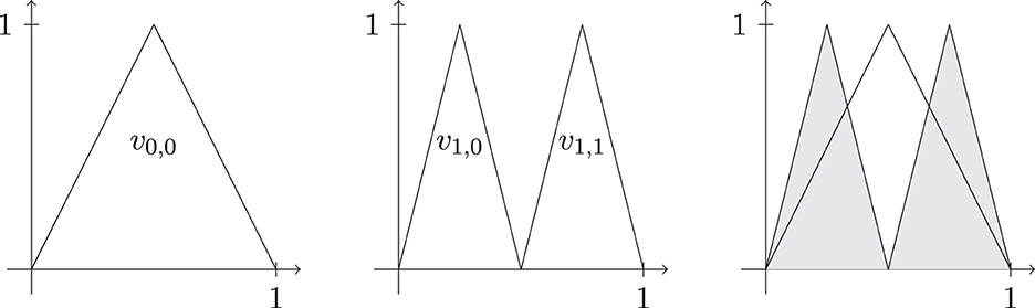
Figure 1. Univariate hierarchical Faber basis on [0, 1] for levels j ∈ {0, 1} and their union.

Remark 4.5. We need to formulate the definition of the Kolmogorov widths to demonstrate some relations with approximative characteristics considered here. For a compact set F↪X of a Banach space X, we define the Kolmogorov widths as follows:

$d_m(F,X):\text{}=\underset{{\left\{u_i\right\}}_{i=1}^m\subset X}{\inf }\underset{f\in F}{\sup }\underset{c_i}{\inf }\Vert f-{\displaystyle \sum _{i=1}^m{c}_i}{u}_i|X\Vert ,m=1,2,\dots ,$

and

$d_0(\text{F},X):={\displaystyle \underset{f\in \text{F}}{sup}}\left|\right|f\left|X\right||.$

Clearly, considering F as the unit ball in $S_{p,\theta }^{1/p}B({\left[0,1\right]}^d)$ with θ ≤ min{p, 1} and $X=L_{\infty }({\left[0,1\right]}^d)$ then

$d_m(S_{p,\theta }^{1/p}B({\left[0,1\right]}^d),L_{\infty }({\left[0,1\right]}^d))\nrightarrow 0$

by Lemma 4.4.

5. The decay of the Faber coefficients

Now we are ready for proving our main tool: an assertion about the decay of the Faber coefficients of functions from $S_{p,min\left\{p,1\right\}}^{1/p}B({ℝ}^d)$ . In order to do so we need to define the following space of doubly indexed sequences.

Definition 5.1. Let 0 < p, θ ≤ ∞ and r ≥ 1/p.

(i) The sequence space $s_{p,\theta }^{r}b$ is the collection of all doubly indexed sequences ${\left\{{\text{λ}}_{j,k}\right\}}_{j\in {\mathbb{N}}_{-1}^d,k\in {\mathbb{Z}}^d}$ such that

$\Vert {\text{λ}}_{j,k}|s_{p,\theta }^{r}b\Vert :\text{}={\left[{\displaystyle \sum _{j\in {\mathbb{N}}_{-1}^d}{2}^{|j{|}_1(r-1/p)\theta }}{\left({\displaystyle \sum _{k\in \mathbb{Z}}|}{\text{λ}}_{j,k}{|}^p\right)}^{\theta /p}\right]}^{1/\theta }$

is finite (with the usual modification if max{p, θ} = ∞).

(ii) Let Ω ⊂ ℝ^d be a compact domain. We define the index set 𝔻_j(Ω) to be the set of all k ∈ ℤd such that x_j,k ∈ Ω. The space $s_{p,\theta }^{r}b(\text{Ω})$ is defined as the space of all doubly indexed sequences ${\left\{{\text{λ}}_{j,k}\right\}}_{j\in {\mathbb{N}}_{-1}^d,k\in D_j(\text{Ω})}$ such that

$\Vert {\text{λ}}_{j,k}|s_{p,\theta }^{r}b(\text{Ω})\Vert :\text{}={\left[{\displaystyle \sum _{j\in {\mathbb{N}}_{-1}^d}{2}^{|j{|}_1(r-1/p)\theta }}{\left({\displaystyle \sum _{k\in {\text{𝔻}}_j\left(\text{Ω}\right)}|}{\text{λ}}_{j,k}{|}^p\right)}^{\theta /p}\right]}^{1/\theta }$

is finite (with the usual modification if max{p, θ} = ∞).

Remark 5.2. (i) In case Ω = [0, 1]^d we have 𝔻_j(Ω) = 𝔻_j, which was defined right before (2.4). In a certain sense the elements of $s_{p,\theta }^{r}b(\text{Ω})$ are restrictions of elements in $s_{p,\theta }^{r}b$ to indices related to Ω. (ii) These sequence spaces already appeared in [[23], Def. 2.1, 3.2]. Let 0 < p, θ ≤ ∞ and r ∈ ℝ. The spaces $s_{p,\theta }^{r}b$ and $s_{p,\theta }^{r}b(\text{Ω})$ are Banach spaces if min{p, θ}≥1. In case min{p, θ} < 1 the space $s_{p,\theta }^{r}b$ is a quasi-Banach space. Moreover, if u: = min{p, θ, 1} it is a u-Banach space, i.e.,

$\left|\right|\text{λ}+\mu \left|s_{p,\theta }^{r}b\right|{|}^u\le \left|\right|\text{λ}\left|s_{p,\theta }^{r}b\right|{|}^u+\left|\right|\mu \left|s_{p,\theta }^{r}b\right|{|}^u,\text{\hspace{1em}λ},\mu \in s_{p,\theta }^{r}b.$

Here is the first main result.

Proposition 5.3. Let 1/2 ≤ p ≤ ∞. Then there exists a constant c > 0 (independent of f) such that

$\begin{array}{ll}||d_{j,k}^2(f){|s}_{p,\infty }^{1/p}b||\le c||f{|S}_{p,min\left\{p,1\right\}}^{1/p}B({ℝ}^d)||& (5.1)\end{array}$

for all $f\in S_{p,min\left\{p,1\right\}}^{1/p}B({ℝ}^d)$.

Proof. Let us put u = min{p, 1}. We make use of the decomposition (2.3) in a slightly modified way. For fixed $j\in {\mathbb{N}}_{-1}^d$ we write $f=\sum _{\ell \in {\mathbb{Z}}^d}{f}_{j+\ell }$. Putting this into (5.1) and using the u-triangle inequality yields

$\begin{array}{l}\Vert d_{j,k}^2(f)|s_{p,\infty }^{1/p}b{\Vert }^u\asymp \underset{j\in {\mathbb{N}}_{-1}^d}{\sup }{2}^{u|j{|}_1/p}\Vert {\displaystyle \sum _{k\in \mathbb{Z}}{d}_{j,k}^2}(f){\chi }_{j,k}(x){\Vert }_p^u\\ \le \underset{j\in {\mathbb{N}}_{-1}^d}{\sup }{2}^{u|j{|}_1/p}{\displaystyle \sum _{\ell \in {\mathbb{Z}}^d}\Vert }{\displaystyle \sum _{k\in \mathbb{Z}}{d}_{j,k}^2}(f_{j+\ell }){\chi }_{j,k}(x){\Vert }_p^u.\end{array}$

Applying Lemma 3.5 we obtain

$\begin{array}{l}\Vert d_{j,k}^2(f)|s_{p,\infty }^{1/p}b{\Vert }^u\lesssim \underset{j\in {\mathbb{N}}_{-1}^d}{\sup }{\displaystyle \sum _{\ell \in {\mathbb{Z}}^d}{2}^{u|j+\ell {|}_1/p}}\Vert f_{j+\ell }{\Vert }_p^u\\ {\displaystyle \prod _{i=1}^d{2}^{-u{\ell }_i/p}}\min \{2^{2u{\ell }_i},1\}\max \{2^{u{\ell }_i/p},1\}\\ \lesssim ({\displaystyle \sum _{\ell \in {\mathbb{Z}}^d}{2}^{u|j+\ell {|}_1/p}}\Vert f_{j+\ell }{\Vert }_p^u)\\ \underset{\ell \in {\mathbb{Z}}^d}{\sup }{\displaystyle \prod _{i=1}^d{2}^{-u{\ell }_i/p}}\min \{2^{2u{\ell }_i},1\}\max \{2^{u{\ell }_i/p},1\}\\ \lesssim \Vert f|S_{p,u}^{1/p}B({ℝ}^d){\Vert }^u,\end{array}$

since the sup stays finite since 1/2 ≤ p ≤ ∞.

As a direct consequence we have the following restricted version.

Corollary 5.4. Let 1/2 ≤ p ≤ ∞. Then there exists a constant c > 0 such that

$\begin{array}{l}||d_{j,k}^2(f){|s}_{p,\infty }^{1/p}b(\text{Ω})||\le c||f{|S}_{p,min\left\{p,1\right\}}^{1/p}B(\text{Ω})||\end{array}$

for all $f\in S_{p,min\left\{p,1\right\}}^{1/p}B(\text{Ω})$.

Proof. Assume $f\in S_{p,min\left\{p,1\right\}}^{1/p}B(\text{Ω})$. Then, by Definition 4.3 there is a $g\in S_{p,min\left\{p,1\right\}}^{1/p}B({ℝ}^d)$ with g|_Ω = f. By Proposition 5.3 we obtain

$||d_{j,k}^2(g)|s_{p,\infty }^{1/p}b||\le c|\left|g\right|S_{p,min\left\{p,1\right\}}^{1/p}B({ℝ}^d)\left|\right|.$

Since $d_{j,k}^2(g)=d_{j,k}^2(f)$ for $j\in {\mathbb{N}}_{-1}^d$ and k ∈ 𝔻_j(Ω) we have

$||d_{j,k}^2(f)|s_{p,\infty }^{1/p}b(\text{Ω})||\le ||d_{j,k}^2(g)|s_{p,\infty }^{1/p}b||$

we obtain

$||d_{j,k}^2(f)|s_{p,\infty }^{1/p}b(\text{Ω})||\le c|\left|g\right|S_{p,min\left\{p,1\right\}}^{1/p}B(ℝd)\left|\right|.$

The last inequality holds for every extension g of f. Taking the infimum yields the result.

The last corollary can be interpreted as a generalization of [[2], Proposition 3.4] to the limiting smoothness case r = 1/p. Related results concerning non-limiting smoothness were obtained in [1, 5, 27].

6. Application for sampling recovery in L_q with q < ∞

In this section, we would like to apply the Faber embedding in Corollary 5.4 for sampling recovery on the unit cube Ω = [0, 1]^d. As we have shown in Lemma 4.4, we cannot expect an error decay of a sampling recovery operator in the worst case when we measure the error in $L_{\infty }({\left[0,1\right]}^d)$. Hence, we focus on the recovery in $L_q({\left[0,1\right]}^d)$ with q < ∞. Based on the Faber representation, we will use a sparse grid truncation in order to obtain a recovery operator. Let

$\begin{array}{ll}{I}_{n}f={\displaystyle \sum _{|j{|}_1\le n}}{\displaystyle \sum _{k\in {𝔻}_j}}{d}_{j,k}^2(f)v_{j,k}& (6.1)\end{array}$

with the notation from Section 2.

Lemma 6.1. The following estimates hold true for α > 0

(i)

$\begin{array}{l}{\displaystyle \sum _{|j{|}_1>n}}{2}^{-\alpha |j{|}_1}\asymp 2^{-\alpha n}{n}^{d-1}\mathrm{and}\end{array}$

(ii)

$\begin{array}{l}{\displaystyle \sum _{|j{|}_1\le n}}{2}^{|j{|}_1}\asymp 2^n{n}^{d-1}.\end{array}$

Proof. We refer to [[28], p. 10, Lemma D].

We first consider the case where p = q.

Theorem 6.1. Let 1/2 ≤ p < ∞. Then there is a constant C > 0 (independent of n and f) such that

$\left|\right|f-I_{n}f|{|}_p\le C{2}^{-n/p}{n}^{(d-1)/min\left\{p,1\right\}}||f{|S}_{p,min\left\{p,1\right\}}^{1/p}B({\left[0,1\right]}^d)||$

holds for all n ∈ ℕ.

Proof. The representation in (2.4) allows us to express and estimate the error by u = min{p, 1}

$\begin{array}{l}\Vert f-I_{n}f{\Vert }_p^u=\Vert {\displaystyle \sum _{|j{|}_1>n}{\displaystyle \sum _{k\in {\text{D}}_j}{d}_{j,k}^2}}(f)v_{j,k}{\Vert }_p^u\\ \le {\displaystyle \sum _{|j{|}_1>n}\Vert }{\displaystyle \sum _{k\in {\text{𝔻}}_j}{d}_{j,k}^2}(f)v_{j,k}{\Vert }_p^u{2}^{u|j{|}_1/p}{2}^{-u|j{|}_1/p}\\ \le {(\underset{j}{\sup }{2}^{|j{|}_1/p}\Vert {\displaystyle \sum _{k\in {\text{𝔻}}_j}{d}_{j,k}^2}(f)v_{j,k}{\Vert }_p)}^u{\displaystyle \sum _{|j{|}_1>n}{2}^{-u|j{|}_1/p}}.\end{array}$

Finally applying Proposition 5.3 or Corollary 5.4 yields

$\begin{array}{l}\Vert f-I_{n}f{\Vert }_p^u\lesssim \Vert d_{j,k}^2(f)|s_{p,\infty }^{1/p}b([0,1]d){\Vert }^u{\displaystyle \sum _{|j{|}_1>n}{2}^{-u|j{|}_1/p}}\\ \lesssim 2^{-un/p}{n}^{d-1}\Vert f|S_{p,\min \{p,1\}}^{1/p}B([0,1]d){\Vert }^u,\end{array}$

where the sum is estimated by Lemma 6.1.

Remark 1. A one-dimensional version of the above result has been proven by Oswald [19] about four decades ago. Dũng proved in [[17], Theorem 3.2] that a related result for slightly different Besov-type function spaces, especially not including the case p = 1/2.

In the situation p < q, we loose in the main rate. This phenomenon has been observed earlier in the literature [see [6]]. We will use Jawerth-Franke type embeddings to improve the order of the logarithmic term.

Theorem 6.2. Let 1/2 ≤ p < q < ∞. Then

$\left|\right|f-I_{n}f|{|}_q\le C{2}^{-n/q}{n}^{(d-1)/q}|\left|f\right|S_{p,min\left\{p,1\right\}}^{1/p}B({\left[0,1\right]}^d)\left|\right|.$

Proof. Using Jawerth-Franke I (see Lemma 4.2), we obtain

$\begin{array}{l}\Vert f-I_{n}f{\Vert }_q\lesssim \Vert f-I_{n}f|S_{p,q}^{1/p-1/q}B\left({[0,1]}^d\right)\Vert \hfill \\ \lesssim {\left({\displaystyle \sum }_{|j{|}_1>n}{2}^{q|j{|}_1[1/p-1/q]}{\Vert {\displaystyle \sum }_{k\in {𝔻}_j}{d}_{j,k}^2(f){\chi }_{j,k}\Vert }_p^q\right)}^{1/q}\hfill \\ \lesssim \left[\underset{j\in {\mathbb{N}}_{-1}^d}{\sup }{2}^{|j{|}_1/p}{\Vert {\displaystyle \sum }_{k\in {𝔻}_j}{d}_{j,k}^2(f){\chi }_{j,k}\Vert }_p\right]{\left({\displaystyle \sum }_{|j{|}_1>n}{2}^{-|j{|}_1}\right)}^{1/q},\hfill \end{array}$

where we used the inverse Faber characterization for spaces with positive smoothness [cf. [1], Theorem 4.18]. This reference deals with the ℝ^d case but can be easily extended by standard arguments as shown, for instance, in the proof of Corollary 5.4 or following the arguments in [[1], Theorem 4.25] to the unit cube setting. Finally applying Proposition 5.3 yields

$\begin{array}{l}\begin{array}{cc}\left|\right|f-I_{n}f|{|}_q& \lesssim 2^{-n/q}{n}^{(d-1)/q}\left|\right|f\left|S_{p,min\left\{p,1\right\}}^{1/p}B({\left[0,1\right]}^d)\right||.\end{array}\end{array}$

Let us now deal with the space $S_{1,\infty }^{1}F({\left[0,1\right]}^d)$, which is embedded into C([0, 1]^d), as shown in Lemma 4.2, (iiic). By Jawerth-Franke embedding II [(Lemma 4.2, (iic)], we even know that for every 1 < p < ∞, we have $S_{1,\infty }^{1}F({\left[0,1\right]}^d)\hookrightarrow S_{p,1}^{1/p}B({\left[0,1\right]}^d)$. As a direct corollary of Theorems 6.1 and 6.2, we make the new observations.

Theorem 6.3. (i) It holds for any small ε > 0

$\left|\right|f-I_{n}f\left|{|}_1{\lesssim }_{\epsilon }{2}^{-n(1-\epsilon )}\right|\left|f\right|S_{1,\infty }^{1}F({\left[0,1\right]}^d)\left|\right|.$

(ii) For any 1 < q < ∞ we have

$\left|\right|f-I_{n}f|{|}_q\lesssim 2^{-n/q}{n}^{(d-1)/q}|\left|f\right|S_{1,\infty }^{1}F({\left[0,1\right]}^d)\left|\right|.$

Proof. By the embedding $S_{1,\infty }^{1}F({\left[0,1\right]}^d)\hookrightarrow S_{p,1}^{1/p}B({\left[0,1\right]}^d)$ for p > 1, we may apply Theorem 6.2 to obtain the result. For (i), we simply choose small q > 1 and use the fact that the L_q-norm dominates the L₁-norm. Clearly, the logterm can be dropped in this regime.

6.1. Sampling widths

Let us focus our considerations toward the problem of optimal sampling recovery. We compare the number m of samples to the resulting error in an algorithm and call the quantity

$\begin{array}{l}\begin{array}{l}{\varrho }_m(S_{p,\theta }^{r}A({[0,1]}^d),L_q({[0,1]}^d))\hfill \\ :=\underset{\begin{array}{c}{X}_m\subset {[0,1]}^d,|X_m|=m\\ \phi :{ℂ}^m\to L_q({[0,1]}^d)\end{array}}{\inf }\underset{||f|S_{p,\theta }^{r}A({[0,1]}^d)||\le 1}{\sup }||f-\phi (f(X_m))L_q({[0,1]}^d)||,\hfill \\ \hfill \end{array}\end{array}$

the m-th sampling width. If, in addition, the mapping $\phi :{ℂ}^n\to L_q({\left[0,1\right]}^d)$ is linear, then we obtain the linear sampling widths

$\begin{array}{l}{\varrho }_m^{lin}\left(S_{p,\theta }^{r}A\left({[0,1]}^d\right),L_q\left({[0,1]}^d\right)\right)\\ :=\underset{\begin{array}{c}{X}_m\subset {[0,1]}^d,|X_m|=m\\ \phi :{ℂ}^m\to L_q({[0,1]}^d)\\ linear\end{array}}{\inf }\underset{||f|S_{p,\theta }^{r}A({[0,1]}^d)||\le 1}{\sup }||f-\phi \left(f(X_m))L_q({[0,1]}^d\right)||,\end{array}$

where A ∈ {B, F}. Therefore, according to the definitions mentioned above, we have

$\begin{array}{l}{\varrho }_m(S_{p,\theta }^{r}A({\left[0,1\right]}^d),L_q({\left[0,1\right]}^d))\le {\varrho }_m^{\text{lin}}(S_{p,\theta }^{r}A({\left[0,1\right]}^d),L_q({\left[0,1\right]}^d)).\end{array}$

In the next theorems, we apply the linear algorithm I_nf [cf. (6.1)] to obtain upper bounds for ${\varrho }_m^{\text{lin}}$ and ϱ_m.

Theorem 6.4. Let 1/2 ≤ p < ∞. Then

$\begin{array}{l}{\varrho }_m^{\text{lin}}(S_{p,min\left\{p,1\right\}}^{1/p}B({\left[0,1\right]}^d),L_p({\left[0,1\right]}^d))\lesssim m^{-1/p}{({log}^{d-1}m)}^{1/p+1/min\left\{p,1\right\}}\end{array}$

for all m ∈ ℕ.

Proof. The upper bound is due to Theorem 6.1 recognizing that the algorithm I_n in (6.1) samples f in m ≍ 2ⁿn^d−1 nodes. This can be trivially checked by applying Lemma 6.1, (ii). For the sake of completeness, we refer to [[1], Section 5.1] where further properties of this operator were studied.

Theorem 6.5. Let 1/2 ≤ p < q < ∞. Then

(i)

${\varrho }_m^{\text{lin}}(S_{p,min\left\{p,1\right\}}^{1/p}B({\left[0,1\right]}^d),L_q({\left[0,1\right]}^d))\lesssim m^{-1/q}{({log}^{d-1}m)}^{2/q}$

and

(ii)

${\varrho }_m^{\text{lin}}(S_{1,\infty }^{1}F({\left[0,1\right]}^d),L_q({\left[0,1\right]}^d))\lesssim m^{-1/q}{({log}^{d-1}m)}^{2/q}$

for all m ∈ ℕ.

Proof. The upper bound in (i) is due to Theorem 6.2 taking the number of sampling nodes into account, see Theorem 6.4. The upper bound in (ii) is due to Theorem 6.3.

6.2. Lower bounds

The linear width of class F in a normed space X has been introduced by Tikhomirov [29] more than 60 years ago. It is defined by

${\text{λ}}_m(F,X):\text{}=\underset{\begin{array}{c}A:X\to X\text{ linear}\\ \text{rank\hspace{0.05em}}A\le m\end{array}}{\inf }\underset{f\in F}{\sup }\Vert f-A(f)|X\Vert .$

Romanyuk [30, 31] proved for F, the unit ball in $S_{p,1}^{r}B({\left[0,1\right]}^d)$, that in case 1 ≤ p ≤ q ≤ 2 and q > 1

$\begin{array}{l}{\text{λ}}_m(S_{p,\theta }^{1/p}B([0,1]d),L_q([0,1]d))\ge d_m(S_{p,\theta }^{1/p}B([0,1]d),L_q([0,1]d))\\ \gtrsim {(m^{-1}{\log }^{d-1}m)}^{1/q}.& (6.2)\end{array}$

We obtain the following lower bounds for the (linear) sampling widths.

Theorem 6.6. (i) Let 1 ≤ p ≤ q < ∞. Then we have

${\varrho }_m(S_{p,1}^{1/p}B({\left[0,1\right]}^d),L_q({\left[0,1\right]}^d))\gtrsim m^{-1/q}.$

(ii) If, additionally, 1 ≤ p ≤ q ≤ 2 and q > 1, then

${\varrho }_m^{\text{lin}}(S_{p,1}^{1/p}B({[0,1]}^d),L_q({[0,1]}^d))\gtrsim {(m^{-1}{\log }^{d-1}m)}^{1/q}.$

Proof. The result in (ii) follows immediately from (6.2). For the lower bound in (i), we use a fooling function that is constructed as the simple tensor function, containing the univariate fooling function obtained from [32] in the first direction smooth compactly supported (bump) functions in all remaining directions. We obtain our result by considering that all corresponding norms have product properties related to simple tensor functions.

7. Outlook and discussion

In this article, we have shown that for the sampling recovery problem the compact embedding into $L_{\infty }({\left[0,1\right]}^d)$ is not necessary. There are several relevant multivariate function classes that fall under this scope, such as limiting mixed Besov and Triebel-Lizorkin spaces with smoothness r = 1/p and further parameter conditions to ensure the embedding into the class of continuous functions. We were able to give upper bounds for the sampling widths in $L_q({\left[0,1\right]}^d)$ with q < ∞, which are sharp in the polynomial main rate. As for the right order of the logarithm, the situation is completely open.

Let us comment on the particular case of L₁-smoothness spaces. Smoothness spaces built upon $L_1({\left[0,1\right]}^d)$ with smoothness r = 1 play an important role in numerical integration. This includes, for instance, the space $S_1^{1}W({\left[0,1\right]}^d)$ defined using weak derivatives. This space cannot be described using Fourier analytical means and is therefore difficult to handle. However, these spaces are considered in the scope of this article since we also have r = 1/p and a non-compact embedding into $L_{\infty }({\left[0,1\right]}^d)$. A Faber characterization is shown, similar to above, including

$\begin{array}{ll}{\displaystyle \underset{j\in {\mathbb{N}}_{-1}^d}{sup}}{\displaystyle \sum _{k\in {\mathbb{Z}}^d}}\left|d_{j,k}^2(f)\right|\lesssim \left|f{S}_1^{1}W({ℝ}^d)\right|.& (7.1)\end{array}$

In particular, this would imply the following so-called sampling inequality

${\displaystyle \sum _{k\in {\mathbb{Z}}^d}}\left|f(k)\right|\lesssim ||f{S}_1^{1}W({ℝ}^d)||.$

This extends the result in [[33], Prop. 2] in several directions. On the one hand, we consider the multivariate case, and on the other hand, the space $S_1^{1}W({ℝ}^d)$ is larger than $S_{1,1}^{1}B({ℝ}^d)$.

Having (7.1) at hand, the following slightly sharper version of Theorem 6.3 is immediate.

Theorem 7.1. For any 1 ≤ q < ∞, we have

$\left|\right|f-I_{n}f|{|}_q\lesssim 2^{-n/q}{n}^{(d-1)/q}||f{S}_1^{1}W({\left[0,1\right]}^d)||.$

A proper Fourier analytical replacement of the spaces $S_1^{1}W({\left[0,1\right]}^d)$ are the spaces $S_{1,q}^{1}F({\left[0,1\right]}^d)$. However, these spaces are not really comparable, especially when q = ∞. Using the methods in [[34], Theorem 1.9], there is strong evidence for proving a version of (7.1) also for the spaces $S_{1,\infty }^{1}F({ℝ}^d)$. This would imply a version of Theorem 7.1. By well-known arguments, a cubature formula with performance

$\left|{\displaystyle {\int }_{{[0,1]}^d}f\left(x\right)dx-}{\displaystyle \sum _{i=1}^N{\lambda }_{i}f(x^i)}\right|\lesssim N^{-1}{(\log N)}^{2(d-1)}\Vert f|S_{1,\infty }^{1}F({[0,1]}^d)\Vert$

can be constructed by integrating the approximand. Note that there were efforts made in the literature to treat such limiting cases, see, for instance [[35], Cor. 6.5]. Suboptimal bounds were proven there. Note that results for such limiting cases are related to the Kokhsma-Hlawka inequality, showing that QMC-cubature in $S_1^{1}W({\left[0,1\right]}^d)$ is related to the star discrepancy of the cubature nodes.

Data availability statement

The original contributions presented in the study are included in the article/supplementary material, further inquiries can be directed to the corresponding author.

Author contributions

All authors listed have made a substantial, direct, and intellectual contribution to the work and approved it for publication.

Funding

SS was supported by the German Academic Exchange Service (DAAD, Grant 57588362) and by the Philipp Schwartz Initiative of the Alexander von Humboldt Foundation.

Acknowledgments

The authors would like to thank the referees for their useful remarks for improving the quality of this manuscript. Additionally, the authors thank Winfried Sickel and Dinh Dũng for discussion and their comments on earlier versions of this manuscript.

Conflict of interest

The authors declare that the research was conducted in the absence of any commercial or financial relationships that could be construed as a potential conflict of interest.

Publisher's note

All claims expressed in this article are solely those of the authors and do not necessarily represent those of their affiliated organizations, or those of the publisher, the editors and the reviewers. Any product that may be evaluated in this article, or claim that may be made by its manufacturer, is not guaranteed or endorsed by the publisher.

References

1. Byrenheid G. Sparse representation of multivariate functions based on discrete point evaluations [Dissertation]. Institut für Numerische Simulation; Universität Bonn, Bonn, Germany (2018).

Google Scholar

2. Hinrichs A, Markhasin L, Oettershagen J, Ullrich T. Optimal quasi-Monte Carlo rules on order 2 digital nets for the numerical integration of multivariate periodic functions. Numer Math. (2016) 134:163–96. doi: 10.1007/s00211-015-0765-y

CrossRef Full Text | Google Scholar

3. Kempka H, Schneider C, Vybiral J. Path regularity of Brownian motion and Brownian sheet. Constr Approx. (2022). doi: 10.1007/s00365-023-09647-z

CrossRef Full Text | Google Scholar

4. Triebel H. Bases in Function Spaces, Sampling, Discrepancy, Numerical Integration. Vol. 11 of EMS Tracts in Mathematics. Zürich: European Mathematical Society (EMS) (2010). doi: 10.4171/085

CrossRef Full Text | Google Scholar

5. Triebel H. Faber Systems and Their Use in Sampling, Discrepancy, Numerical Integration. EMS Series of Lectures in Mathematics. Zürich: European Mathematical Society (EMS) (2012). doi: 10.4171/107

CrossRef Full Text | Google Scholar

6. Dũng D, Temlyakov VN, Ullrich T. Hyperbolic Cross Approximation. In: Tikhonov S, , editor. Advanced Courses in Mathematics. CRM Barcelona. Cham: Birkhäuser; Springer (2018). doi: 10.1007/978-3-319-92240-9

CrossRef Full Text | Google Scholar

7. Krieg D, Ullrich M. Function values are enough for L₂-approximation. Found Comp Math. (2021) 21:1141–51. doi: 10.1007/s10208-020-09481-w

CrossRef Full Text | Google Scholar

8. Nagel N, Schäfer M, Ullrich T. A new upper bound for sampling numbers. Found Comp Math. (2022) 22:445–68. doi: 10.1007/s10208-021-09504-0

CrossRef Full Text | Google Scholar

9. Bartel F, Schäfer M, Ullrich T. Constructive subsampling of finite frames with applications in optimal function recovery. Appl Comput Harmon Anal. (2023) 65:209–248. doi: 10.1016/j.acha.2023.02.004

CrossRef Full Text | Google Scholar

10. Krieg D, Ullrich M. Function values are enough for L₂-approximation. II. J Complex. (2021) 66:14. doi: 10.1016/j.jco.2021.101569

CrossRef Full Text | Google Scholar

11. Dolbeault M, Krieg D, Ullrich M. A sharp upper bound for sampling numbers in L₂. Appl Comput Harmon Anal. (2023) 63:113–34. doi: 10.1016/j.acha.2022.12.001

CrossRef Full Text | Google Scholar

12. Temlyakov VN, Ullrich T. Approximation of functions with small mixed smoothness in the uniform norm. J Approx Theory. (2022) 277:105718. doi: 10.1016/j.jat.2022.105718

CrossRef Full Text | Google Scholar

13. Temlyakov V, Ullrich T. Bounds on Kolmogorov widths and sampling recovery for classes with small mixed smoothness. J Complex. (2021) 67:101575. doi: 10.1016/j.jco.2021.101575

CrossRef Full Text | Google Scholar

14. Temlyakov V. On optimal recovery in L₂. J Complex. (2021) 65:101545. doi: 10.1016/j.jco.2020.101545

CrossRef Full Text | Google Scholar

15. Jahn T, Ullrich T, Voigtlaender F. Sampling numbers of smoothness classes via ℓ¹-minimization. J Complex. (2022). doi: 10.48550/arXiv.2212.00445

CrossRef Full Text | Google Scholar

16. Bungartz HJ, Griebel M. Sparse grids. Acta Numer. (2004) 13:147–269. doi: 10.1017/S0962492904000182

CrossRef Full Text | Google Scholar

17. Dũng D. B-spline quasi-interpolant representations and sampling recovery of functions with mixed smoothness. J Complex. (2011) 27:541–67. doi: 10.1016/j.jco.2011.02.004

CrossRef Full Text | Google Scholar

18. Ullrich T. Smolyak's algorithm, sparse grid approximation and periodic function spaces with dominating mixed smoothness (PhD thesis). Friedrich-Schiller-Universität Jena, Jena, Germany (2007).

Google Scholar

19. Oswald P. L^p-Approximation durch Reihen nach dem Haar-Orthogonalsystem und dem Faber-Schauder-System. J Approx Theory. (1981) 33:1–27. doi: 10.1016/0021-9045(81)90086-1

CrossRef Full Text | Google Scholar

20. Schmeisser HJ, Triebel H. Topics in Fourier Analysis and Function Spaces. A Wiley-Interscience Publication. Chichester: John Wiley & Sons, Ltd. (1987).

Google Scholar

21. Faber G. Über stetige Funktionen. Math Ann. (1909) 66:81–94. doi: 10.1007/BF01450912

CrossRef Full Text | Google Scholar

22. Ullrich T. Function spaces with dominating mixed smoothness, characterization by differences. Tech Rep Jenaer Schriften zur Math Inform. (2006).

Google Scholar

23. Vybiral J. Function spaces with dominating mixed smoothness. Dissert Math. (2006) 436:73. doi: 10.4064/dm436-0-1

CrossRef Full Text | Google Scholar

24. Hansen M, Vybíral J. The Jawerth–Franke embedding of spaces with dominating mixed smoothness. Georg Math J. (2009) 16:667–82. doi: 10.1515/GMJ.2009.667

CrossRef Full Text | Google Scholar

25. Mayer S, Ullrich T. Entropy numbers of finite dimensional mixed-norm balls and function space embeddings with small mixed smoothness. Constr Approx. (2021) 53:249–79. doi: 10.1007/s00365-020-09510-5

CrossRef Full Text | Google Scholar

26. Triebel H. Theory of Function Spaces. Modern Birkhäuser Classics. Basel: Birkhäuser/Springer Basel AG (2010).

Google Scholar

27. Ullrich T. Optimal cubature in Besov spaces with dominating mixed smoothness on the unit square. J Complex. (2014) 30:72–94. doi: 10.1016/j.jco.2013.09.001

CrossRef Full Text | Google Scholar

28. Temlyakov V. Approximation of functions with bounded mixed derivative. Proc Steklov Inst Math. (1986) 20:173

Google Scholar

29. Tikhomirov VM. Diameters of sets in functional spaces and the theory of best approximations. Russ Math Surv. (1960) 15:75–111. doi: 10.1070/RM1960v015n03ABEH004093

CrossRef Full Text | Google Scholar

30. Romanyuk AS. Approximation of the Besov classes of periodic functions of several variables in the space L_q. Ukr Math J. (1991) 43:1297–306. doi: 10.1007/BF01061817

CrossRef Full Text | Google Scholar

31. Romanyuk AS. Kolmogorov and trigonometric widths of the Besov classes $B_{p,\theta }^r$ of multivariate periodic functions. Sb Math. (2006) 197:69–93. doi: 10.1070/SM2006v197n01ABEH003747

CrossRef Full Text | Google Scholar

32. Novak E, Triebel H. Function spaces in Lipschitz domains and optimal rates of convergence for sampling. Constr Approx. (2006) 23:325–50. doi: 10.1007/s00365-005-0612-y

CrossRef Full Text | Google Scholar

33. Schmeisser HJ, Sickel W. Sampling theory and function spaces. In: Applied Mathematics Reviews. Vol. 1. River Edge, NJ: World Science Publication (2000). p. 205–84. doi: 10.1142/9789812792686_0008

CrossRef Full Text | Google Scholar

34. Garrigós G, Seeger A, Ullrich T. Haar frame characterizations of Besov-Sobolev spaces and optimal embeddings into their dyadic counterparts. J Fourier Anal Appl. (2023) 29:39. doi: 10.1007/s00041-023-10013-7

CrossRef Full Text | Google Scholar

35. Ullrich M, Ullrich T. The role of Frolov's cubature formula for functions with bounded mixed derivative. SIAM J Numer Anal. (2016) 54:969–93. doi: 10.1137/15M1014814

CrossRef Full Text | Google Scholar