A nonstandard fitted operator finite difference method for two-parameter singularly perturbed time-delay parabolic problems

1. Introduction

Singular perturbation problems (SPPs) were first established as a research domain in the early 1990's [1] with the development of the boundary-layer idea in viscous flow [2] and has flourished over the last few years. Despite the large amount of studies that have already been done in this thematic area, more relevant and timely research is still ongoing.

Differential equations whose highest order derivative terms are attached with small positive number(s) are called singularly perturbed problems (SPPs). Singularly perturbation problems appearing with two small parameters are said to be two-parameter singularly perturbed problems. A singularly perturbed delay differential equation (SPDDE) is a differential equation in which the highest derivative is multiplied by a small parameter and containing at least one delay term either at the space variable, time variable, or both.

A lot of real-life physical problems are represented by linear or nonlinear differential models or by SPPs whose solution depends on the magnitude of the perturbation parameter. Singularly perturbed problems (SPPs) occur in the modeling of fluid dynamics, elasticity theory, quantum mechanics, reaction diffusion process, chemical reactor theory, plasma dynamics, meteorology, diffraction theory, aerodynamics, modeling of semi-conductors, hydrodynamics, and in several other applied fields [3–6].

Two-parameter singularly perturbed parabolic differential equations with time delay have many applications in different fields, for example, in engineering such as drift diffusion equation of semi conductor modeling [7] and chemical reactor model [8] in fluid dynamics [9].

Friedrichs and Wasow [10] were the first to use the term singular perturbation problems in their seminar at New York. In such problems, there are often narrow transition regions called boundary layers. In these regions, the solution changes rapidly or jumps abruptly and behaves regularly and slowly away from the layers.

For the solution of singular perturbation problems, one may apply the numerical approach or the asymptotic approach. The asymptotic approach provides the qualitative behavior of the problem and gives only a semi-quantitative information. However, the numerical approach provides quantitative information.

To solve singularly perturbed problems numerically (when analytical solutions are not available or more complicated), one can use finite difference methods, finite elements methods, spline approximation methods, and others, but, unless very fine grids are used, standard finite difference methods can not resolve the layers(s) and may not provide a uniformly convergent solution throughout the given domain.

The two non classical finite difference methods (FDMs) used for solving SPPs are fitted mesh methods (FMFDMs) and fitted operator methods (FOFDMs). In this article, we develop a uniformly convergent and accurate non-standard fitted operator finite difference method (NSFOFDM) based on the methodology of Mickens [11].

As the parameters ε and μ in the problem (1) of section (2) tend to zero, the solution will produce boundary layer(s) at x = 0 and x = 1. When μ = 1, problem (1) is convection- diffusion problem [12–14], and in this case, a boundary layer(s) of width O(ε) will occur around the edge x = 0. Again, when μ = 0, we have a parabolic reaction-diffusion problem [15] and thin boundary layers of width $O(\sqrt{\epsilon })$ appear near x = 0 and x = 1. O'Malley [16] introduced singularly perturbed two-parameter problems and examined asymptotic expansion for their solutions. O'Malley [16, 17] identified that the nature of these problems is quite affected by the choice of ratio of μ² to ε.

O'Malley et al. developed numerical methods to improve the accuracy of the asymptotic methods [16]. The class of time-dependent SPPs of convection-diffusion types with two parameter were studied in Munyakazi [18] using the classical finite difference method. Recently, the numerical solution of second-order two-parametric singularly perturbed ordinary differential equations (ODEs) with smooth data [19–32] and non-smooth data [33, 34] were considered.

Some uniformly convergent numerical methods for singularly perturbed time dependent delay differential equations have been developed in Bashier and Patidar, Kaushik et al., Kumar and Kumar, Erdogan and Cen, Cen, Singh et al., Ansari et al., and Kumar and Kumar [35–42].

In Govindarao et al. [43], a first-order uniformly convergent method was developed for two-parameter time dependent SPPs using an upwind finite difference scheme on Shishkin type meshes.

Solving two-parameter SPPs analytically is either more difficult task or the analytical solution does not exist. This is because of the small parameters attached to the highest order terms of the given problem. These attached small parameters exhibit a layer behavior in the solutions. The classical finite difference methods give unstable solution in the layer region. Moreover, the convergence and stability of the solution in numerical part varies according to the small parameters. From the existing literature we have seen, developing a parameter uniformly convergent numerical method for two-parameter singularly perturbed problems is still a challenging task.

The objective of this study is to analyze the solution when the delay is non-zero and the effect of the delay on the boundary layer solution, as well as investigate problems (1)–(2) with smooth data. We are inspired to develop a parameter uniformly convergent numerical scheme to treat a class of second-order two-parameter singularly perturbed time dependent problem (1)–(2). A non-standard fitted operator finite difference method based on the Crank-Nicolson discretization for time variable comprising a non-standard fitted operator finite difference on uniform mesh for spatial variable. The developed scheme is of second order in time and first order in space but has been improved to second order in both variables by using temporal mesh refinement in Section (5) in Tables 4, 5. Moreover, the comparison of the developed scheme with the existing scheme in Kumar and Kumar [44] is investigated in Section (5) in Table 6. The comparison shows that the maximum point-wise error of our scheme is less than the scheme in Kumar and Kumar [44].

This article is organized as follows. We first discuss the qualitative properties such as the bounds of the analytical solution u(x, t) of problem (1–2) and its derivative bounds in Section (2). The numerical scheme of the continuous problem is presented in Section (3). In this section, we also discuss the time discretization, the space discretization, the continuous problem discretization, and bounds of the discrete solution. The stability and convergence analysis of the scheme is presented in Section (4). In Section (5), we provide numerical example to show uniformly convergence of solution and its accuracy. We present the result and conclusions in Section (6).

2. The continuous problem

We consider the following two families of two-parameter singularly perturbed time-delay problem. Our domain $\bar{D}$ = D∪∂D, where D = (0, 1) × (0, T] and ∂D = L_l ∪ L_d ∪ L_r with L_d = [0, 1] × [−γ, 0](delay interval), L_l = {0} × (0, T](left side boundary) and L_r = {1} × (0, T](right side boundary). The governing equation is as follows:

$\begin{array}{ll}Lu(x,t)-u_t(x,t)=-c(x,t)u(x,t-\gamma )+f(x,t),(x,t)\in D,& (1)\end{array}$

$\begin{array}{l}\text{with }u(x,t)={\text{Φ}}_d(x,t),(x,t)\in L_d,\\ u(0,t)={\text{Φ}}_l(t),u(1,t)={\text{Φ}}_r(t),t\in [0,T],& (2)\end{array}$

where Lu(x, t) = εu_xx(x, t) + μa(x, t)u_x(x, t) − b(x, t)u(x, t), 0 < ε ≤ 1 and 0 ≤ μ ≤ 1 are perturbation parameters and γ is a delay parameter. In problem (1–2), we suppose that a(x, t), b(x, t), c(x, t), f(x, t), Φ_l(t), Φ_r(t), and Φ_d(x, t) for $(x,t)\in \overline{D}$ are sufficiently smooth functions such that a(x, t) ≥ α > 0, b(x, t) ≥ β > 0, and c(x, t) ≥ ϒ > 0, independent of the perturbation parameters. At the corners, the regularity and compatibility conditions are

$\begin{array}{l}u(0,0)={\text{Φ}}_l(0),u(1,0)={\text{Φ}}_r(0),u(0,-\gamma )=\\ {\text{Φ}}_l(\gamma ),u(1,-\gamma )={\text{Φ}}_r(-\gamma )\\ \epsilon {({\text{Φ}}_d)}_{xx}(0,0)+\mu a(0,0){({\text{Φ}}_d)}_x(0,0)-b(0,0)({\text{Φ}}_d)(0,0)-\\ {({\text{Φ}}_b)}_t(0,0)=-c(0,0)({\text{Φ}}_d)(0,-\gamma )+f(0,0)\\ \epsilon {({\text{Φ}}_d)}_{xx}(1,0)+\mu a(1,0){({\text{Φ}}_d)}_x(1,0)-b(1,0)({\text{Φ}}_d)(1,0)-\\ {({\text{Φ}}_d)}_t(1,0)(1,0)({\text{Φ}}_d)(1,-\gamma )+f(1,0)\end{array}$

for D = (0, 1) × (0, T], and so that Φ_d (x, t) (initial-boundary data) satisfies appropriate compatibility criteria at the two corners, (0, 0) and (1, 0). Based on the above assumptions, the given problem in (1) possesses a unique solution in the considered domain.

2.1. Some qualitative properties of the continuous problem

In this section, we present some analytical properties of the governing problem (1–2) in one space dimension and defined domain $\bar{D}$.

First, we will state and prove minimum principle and describe derivative bounds for the solution.

Lemma 2.1. The minimum principle for the continuous SPP [44]. Let $\phi (x,t)\in C^{2,1}\bar{D}$. If φ|_∂D ≥ 0 and $\left(L_{\epsilon ,\mu }-\frac{\partial }{\partial t}\right)\phi {|}_D\le 0$, then $\phi {|}_{\bar{D}}\ge 0$.

Proof. Let (x^⋆, t^⋆) be an arbitrary point in a plane, D = (0, 1) × (0, T) such that $\phi (x^{\star },t^{\star })=min{\left\{\phi (x,t)\right\}}_{(x^{\star },t^{\star })\in \bar{D}}$ and again suppose that φ(x^⋆, t^⋆) < 0. Clearly, (x^⋆, t^⋆) ∉ {0, 1} × {0, T} and from the definition of (x^⋆, t^⋆), we have ${\phi }_{xx}(x^{\star },t^{\star })\ge 0,\nabla {\phi }_x(x^{\star },t^{\star })=0,\nabla {\phi }_t(x^{\star },t^{\star })=0$ (applying first and second derivative test for multi-variable functions). Now, we have

$\begin{array}{l}\left(L_{\epsilon ,\mu }-\frac{\partial }{\partial t}\right)\phi {|}_D={\displaystyle \underset{\ge 0}{{\displaystyle \underbrace{\epsilon {\phi }_{xx}(x^{\star },t^{\star })}}}}+{\displaystyle \underset{=0}{{\displaystyle \underbrace{\mu a(x^{\star },t^{\star }){\nabla }_x\phi (x^{\star },t^{\star })}}}}\\ {\displaystyle \underset{\ge 0}{{\displaystyle \underbrace{-b(x^{\star },t^{\star })\phi (x^{\star },t^{\star })}}}}{\displaystyle \underset{=0}{{\displaystyle \underbrace{-{\nabla }_t\phi (x^{\star },t^{\star })}}}}\ge 0.\end{array}$

This is a contradiction. So that our initial assumption φ(x^⋆, t^⋆) < 0 is wrong. Therefore, $\phi (x^{\star },t^{\star }){|}_{\bar{D}}\ge 0$. Since (x^⋆, t^⋆) is arbitrary point, we have φ(x, t) ≥ 0 for all $(x,t)\in \bar{D}$.      □

Lemma 2.2. Bound of the continuous SPP and its derivatives. Let u be the solution of problem (1)–(2) such that u = v + w_L + w_R, where v is the regular component and w_L and w_R are the left and right singular components, respectively [44], and let C be sufficiently large constant which is independent of the perturbation parameters. Then,

$\begin{array}{l}a.\parallel u\parallel \le C.\end{array}$

b. For all non- negative integers i and j (0 ≤ i + 2j ≤ 4), the derivatives of the solution u of problem (1)–(2) satisfy

$\begin{array}{l}\Vert \frac{{\partial }^{i+j}u}{\partial x^i\partial t^j}\Vert \le \{\begin{array}{l}C\frac{1}{{(\sqrt{\epsilon })}^i},\text{\hspace{1em}\hspace{1em} when }\alpha {\mu }^2\le \eta \epsilon \hfill \\ C{\left(\frac{\mu }{\epsilon }\right)}^i{\left(\frac{{\mu }^2}{\epsilon }\right)}^j,\text{\hspace{1em} when }\alpha {\mu }^2\ge \eta \epsilon \hfill \end{array}\end{array}$

$c.\left|w_L(x,t)\right|\le C{e}^{-{\theta }_{L}x},\left|w_R(x,t)\right|\le C{e}^{-{\theta }_R(1-x)}$

where

${\theta }_L=\{\begin{array}{l}\frac{\sqrt{\eta \alpha }}{\sqrt{\epsilon }},\alpha {\mu }^2\le \eta \epsilon ,\hfill \\ \frac{\alpha \mu }{\epsilon },\alpha {\mu }^2\ge \eta \epsilon ,\hfill \end{array}{\theta }_R=\{\begin{array}{l}\frac{\sqrt{\eta a}}{2\sqrt{\epsilon }},\alpha {\mu }^2\le \eta \epsilon \hfill \\ \frac{\eta }{2\mu },\alpha {\mu }^2\ge \eta \epsilon .\hfill \end{array}$

Proof. One can get the proof in Kumar and Kumar and O'Riordan et al. [44, 45].

The singular component and the regular component derivative bounds are justified by the following theorem.

Theorem 2.1. For i, j ∈ 𝕎 = {0, 1, 2, 3, ...}, satisfying 0 ≤ i + 2j ≤ 4, derivative bounds for u are given by

$\Vert \frac{{\partial }^{i+j}v}{\partial x^i\partial t^j}\Vert \le \{\begin{array}{ll}C,\hfill & \text{ when }\alpha {\mu }^2\le \eta \epsilon \hfill \\ C\left(1+{\left(\frac{\epsilon }{\mu }\right)}^{3-i}{\left(\frac{{\mu }^2}{\epsilon }\right)}^j\right),\hfill & \text{ when }\alpha {\mu }^2\ge \eta \epsilon \hfill \end{array}$

Proof. The detail of the proof is in Kumar and Kumar and O'Riordan et al. [44, 45].

3. The numerical scheme

Here, we develop the numerical scheme by discretizing the temporal domain, the spatial domain, and the given singularly perturbed problem in (1)–(2).

3.1. Semi-discrete scheme using temporal discretization

For the discretization of the temporal domain, we divide the given time domain [0, T] using a uniform mesh. We have chosen γ in such a way that T = kγ for some positive integer k > 1. Moreover, if the set D^M is the collection of all mesh points in [0, T] and if $D_{\gamma }^m$ is all mesh points in [−γ, 0], then $D^M=\{t_j=j△t,j=0,1,2,...,M,t_M=T,△t=\frac{T}{M}\}$ and $D_{\gamma }^m=\{t_j=j△t,j=0,1,2,...,m,t_m=\gamma ,△t=\frac{\gamma }{m}\}$, respectively, where M is the number of mesh points in time interval [0, T] and m is the number of mesh points in [−γ, 0]. The continuous problem is semi-discretized using the Crank-Nicolson finite difference method in the temporal direction. The derivation of Crank Niconson scheme for U_t(x, t_j) at (x, j + 1/2) time step is by using Taylor's series expansion for U^j+1 and U^j.

$\begin{array}{l}{U}^{j+1}(x)=U^{j+1/2}(x)+\frac{\text{Δ}t}{2}\frac{\partial U^{j+1/2}(x)}{\partial t}+\\ {\left(\frac{\text{Δ}t}{2}\right)}^2\frac{1}{2!}\frac{{\partial }^2{U}^{j+1/2}(x)}{\partial t^2}+{\left(\frac{\text{Δ}t}{2}\right)}^3\frac{1}{3!}\frac{{\partial }^3{U}^{j+1/2}(x)}{\partial t^3}+...& (3)\end{array}$

$\begin{array}{l}{U}^j(x)=U^{j+1/2}(x)-\frac{\text{Δ}t}{2}\frac{\partial U^{j+1/2}(x)}{\partial t}+\\ {\left(\frac{\text{Δ}t}{2}\right)}^2\frac{1}{2!}\frac{{\partial }^2{U}^{j+1/2}(x)}{\partial t^2}-{\left(\frac{\text{Δ}t}{2}\right)}^3\frac{1}{3!}\frac{{\partial }^3{U}^{j+1/2}(x)}{\partial t^3}+...& (4)\end{array}$

Now, if we subtract (4) from (3), then the term U^j+1/2(x) is eliminated and we obtain

$\begin{array}{l}\frac{U^{j+1}(x)-U^j(x)}{\text{Δ}t}=\frac{\partial U^{j+1/2}(x)}{\partial t}+O{(\text{Δ}t)}^3\end{array}$

and the local truncation error (T^j+1/2(x)) is

$\begin{array}{l}{T}^{j+1/2}(x)=\frac{{(\text{Δ}t)}^3}{24}\frac{{\partial }^3{U}^{j+1/2}(x)}{\partial t^3}+H.O.Ts\text{(higher order terms)}\end{array}$

Rearranging the problem in (1) using the above discritizations, we can write the semi-discretized scheme as

$\begin{array}{l}\frac{u(x,t_{j+1})-u(x,t_j)}{\text{Δ}t}=\epsilon u_{xx}(x,t_{j+1/2})+\mu a(x_i,t_{j+1/2})u_x(x,t_{j+1/2})\\ -b(x,t_{j+1/2})u(x,t_{j+1/2})-f(x,t_{j+1/2})+O\left({(\text{Δ}t)}^3\right)\}\\ +\{\begin{array}{l}-c(x,t_{j+1/2}){\text{Φ}}_d(x)\hfill \\ \text{ for }j=0,1,\cdots ,m\hfill \\ -c(x,t_{j+1/2})u(x,t_{j+1/2-m})\hfill \\ \text{ for }j=m+1,\cdots ,M-1\hfill \end{array}& (5)\end{array}$

where

$\begin{array}{l}u(x,t_{j+1/2})=\frac{u(x,t_{j+1})+u(x,t_j)}{2}+\\ O({(\text{Δ}t)}^3)andf(x,t_{j+1/2})=\frac{f(x,t_{j+1})+f(x,t_j)}{2}+O({(\text{Δ}t)}^3)\end{array}$

Lemma 3.1. Semi-discrete minimum principle. Assume that ${\left[L_{}^{M}U(x)\right]}^{j+1}$ is the discrete operator given in (5) and φ^j+1(x) is any mesh function satisfying ${\phi }^{j+1}(x){|}_{\partial D}\ge 0$ and $\left[L^M\phi {(x)}^{j+1}\right]{|}_D\le 0$ for 0 ≤ j ≤ M, then ${\phi }^{j+1}(x){|}_{\bar{D}}\ge 0$.

Proof. Let s^⋆ ∈ D be any arbitrary point, such that ${\phi }^{j+1}(s^{\star })=\underset{x\in D}{min}{\phi }^{j+1}(x)$. Again, suppose φ^j+1(x) < 0. It is clear that the set $((s^{\star },t_{j+1})\notin \{(0,t_{j+1}),(1,t_{j+1})\}$. By using the concept of first test and second derivative test for multi-variable functions of calculus, we have ${({\phi }_{xx})}^{j+1}(s^{\star })\ge 0,{({\phi }_x)}^{j+1}(s^{\star })=0$. This gives L^Mφ(^s⋆)j+1 > 0 which contradict to the fact that L^Mφ(x)^j+1 ≤ 0. Therefore, ${\phi }^{j+1}(x){|}_{\bar{D}}\ge 0$ is our desire result. □     □

Lemma 3.2. Estimate of local error. Suppose that $||\frac{{\partial }^{k}u(x,t)}{\partial t^k}||\le C,(x,t)\in \overline{D},k=0,1,2.$ The error estimate in temporal direction $e_{j+1}=U^{j+1}(x)-u(x,t_{j+1})$ for sufficiently large constant C is

$\parallel e_{j+1}\parallel \le C{(\text{Δ}t)}^3$

Proof. From the Crank-Nicholson finite difference method of temporal discritization, the fourth order Taylor's series expansion, we have

$\begin{array}{ll}\frac{U^{j+1}(x)-U^j(x)}{\text{Δ}t}=\frac{\partial U^{j+1/2}(x)}{\partial t}+O({(\text{Δ}t)}^3)& (6)\end{array}$

Using Equation 6 into (1)–(2), we get

$L_{\epsilon ,\mu }{u}^{j+1}(x)=u_t^{j+1}(x)+O({(\text{Δ}t)}^3).$

Again, we apply the semi-discrete minimum operator for e_k+1, and then we have

$L_{\epsilon ,\mu }^M{e}^{j+1}(x)=O({(\text{Δ}t)}^3)$

Then, by lemma (3.1) the local error is bounded and given as

$\parallel e_{j+1}\parallel \le C{(\text{Δ}t)}^3$

     □

Lemma 3.3. Estimate of global error. The global error, $E_j=U^j(x)-u(x,t_j$ of the time discretization satisfies

$||E_j{||}_{\infty }\le C{(\text{Δ}t)}^2$

where C is a constant independent of ε, μ, and Δt.

Proof. By using the estimation of local errors, the global error at j + 1 nodal points is given as

$\Vert E_{j+1}\Vert =\Vert {\displaystyle \sum _{\iota =1}^j{e}_{\iota }}\Vert ,j(\text{Δ}t)\le T$

$\begin{array}{l}=\parallel e_1+e_2+e_3+e_4+...+e_j\parallel \\ \le \parallel e_1\parallel +\parallel e_2\parallel +\parallel e_3\parallel +\parallel e_4\parallel +...+\parallel e_j\parallel \\ \le C_1{(\text{Δ}t)}^3+C_2{(\text{Δ}t)}^3+C_3{(\text{Δ}t)}^3+C_4{(\text{Δ}t)}^3+...+C_j{(\text{Δ}t)}^3\\ \le C^{\prime }(j){(\text{Δ}t)}^3\\ \le C^{\prime }\frac{T}{\text{Δ}t}{(\text{Δ}t)}^3=C^{\prime }T{(\text{Δ}t)}^2,becausej\le \frac{T}{\text{Δ}t}\\ \le C{(\text{Δ}t)}^2,where,C=C^{\prime }T\end{array}$

Thus, the semi-discrete scheme is convergent of order two in time.

Lemma 3.4. Let U^j(x) be the semi-discrete solution of (1)–(2). For a certain order of derivative q that depends on the smoothness of data, U^j(x) satisfies the following bound following bound:

$\left|\frac{d^{\xi }{U}^j(x)}{d{x}^{\xi }}\right|\le C\left(1+{\text{Θ}}_1^{\xi }{e}^{-p{\text{Θ}}_{1}x}+{\text{Θ}}_2^{\xi }{e}^{-p{\text{Θ}}_2(1-x)}\right)\Vert , for 0\le \xi \le q$

where p is any real constant such that 0 < p < 1.

Proof. This lemma was proved in Kadalbajoo and Yadaw [46].      □

     □

3.2. Full-discrete scheme using spatial discretization

To discritize the spatial domain, we consider ${\bar{D}}^N$ that denotes the interval [0, 1] and then divide it into N sub-intervals such that

$x_0=0,x_1=x_0+i=h,x_2=x_1+h=2h,\cdots x_N=Nh=1.$

Then, the discretization of the rectangular domain is ${\bar{D}}^{N,M}=({\bar{D}}^N\times {\bar{D}}^M)\cup ({\bar{D}}^N\times {\bar{D}}^m)$, and also the discretization of the boundary data and boundary conditions is $\partial D^{N,M}=L_d^{\text{N, M}}\cup L_l^{\text{N,M}}\cup L_r^{\text{N,M}}$, where $L_d^{\text{N,M}}=$ ${\bar{D}}^N\times {\bar{D}}^m,L_l^{N,M}={\bar{D}}^N\cap L_l$ and $L_r^{\text{N,M}}={\bar{D}}^N\cap L_r$. ${\bar{D}}^m$ denotes the uniform temporal meshes in [−γ, 0]. Again, using the space discretization and the semi-discrete in (5), we can write the full-discrete scheme as

$\begin{array}{l}{\left[L_{}^{N,M}U\right]}_i^j\equiv \frac{u\left(x_i,t_{j+1}\right)-u\left(x_i,t_j\right)}{\text{Δ}t}=\epsilon u_{xx}\left(x_i,t_{j+1/2}\right)+\\ \mu a(x_i,t_{j+1/2})u_x\left(x_i,t_{j+1/2}\right)\\ -b\left(x_i,t_{j+1/2}\right)u\left(x_i,t_{j+1/2}\right)-f\left(x_i,t_{j+1/2}\right)+O\left({(\text{Δ}t)}^3\right)\}\\ +\{\begin{array}{l}-c\left(x_i,t_{j+1/2}\right){\text{Φ}}_d(x_i)\hfill \\ \text{ for} i=0,1,\cdots ,N, j=0,1,\cdots ,m\hfill \\ -c\left(x_i,t_{j+1/2}\right)u\left(x_i,t_{j+1/2-m}\right)\hfill \\ \text{ for} i=0,1,\cdots ,N, j=m+1,\cdots ,M-1\hfill \end{array}& (7)\end{array}$

Next, the resulting discretized equation in (7) can be rearranged using a non-standard fitted operator finite difference method following the steps in Mickens [11].

$\begin{array}{l}{\left[L_{}^{N,M}U\right]}_i^j\equiv \\ \frac{1}{2}\left[\epsilon {\delta }_x^2{U}_i^{j+1}+\mu {a_i}^{j+1}{D}_x^{+}{U}_i^{j+1}-b_i^{j+1}{U}_i^{j+1}+\epsilon {\delta }_x^2{U}_i^j+\mu {a_i}^j{D}_x^{+}{U}_i^j-b_i^j{U}_i^j\right]\\ -D_t{U}_i^{j+1/2}=F_i^{j}i=0,1,2,\cdots ,N-1,j=0,1,2,\cdots ,M-1& (8)\end{array}$

where

$\begin{array}{l}{D}_x^{+}{U}_i^j=\frac{U_{i+1}^j-U_i^j}{h_x},\\ D_t{U}_i^{j+1/2}=\frac{U_i^{j+1}-U_i^j}{\text{Δ}t}{\delta }_x^2{U}_i^j=\left(\frac{U_{i+1}^j-2U_i^j+u_{i-1}^j}{{\varphi }_i^2}\right)\\ D_x^{+}{U}_i^{j+1}=\frac{U_{i+1}^{j+1}-U_i^{j+1}}{h_x},{\delta }_x^2{U}_i^{j+1}=\left(\frac{U_{i+1}^{j+1}-2U_i^{j+1}+u_{i-1}^{j+1}}{{\varphi }_i^2}\right)\end{array}$

and

$\begin{array}{ll}{F}_i^j=\{\begin{array}{l}\frac{1}{2}\left[-c_i^{j+1}{\psi }_{bi}{}^{j+1}-c_i^j{\psi }_{bi}{}^{j+1}+f_i^{j+1}+f_i^j\right],forj=0,1,\cdots ,m\\ \frac{1}{2}\left[-c_i^{j+1}{U}_i{}^{j-m+1}-c_i^j{U}_i{}^{j-m}+f_i^{j+1}+f_i^j\right],\text{ for }j=m+1,\cdots ,M-1\end{array}& (9)\end{array}$

Again, from Munyakazi [18], the denominator function ${\varphi }_i^2$ is given by

${\varphi }_i^2(h,\epsilon ,\mu )\equiv {\varphi }_i^2=\frac{h\epsilon }{\mu a(x_i)}\left(\text{exp}\left(\frac{\mu a(x_i)h}{\epsilon }\right)-1\right)$

Equation 8 can be written in compact form as

$\begin{array}{ll}{\left[L_{}^{N,M}U\right]}_i^j\equiv & {\delta }^{+}{U}_{i+1}^{j+1}+{\delta }^c{U}_i^{j+1}+{\delta }^{-}{U}_{i-1}^{j+1}+{\delta }_1^{+}{U}_{i+1}^j+{\delta }_1^c{U}_i^j+\\ {\delta }_1^{-}{U}_{i-1}^j=F_i^j& (10)\end{array}$

where

$\begin{array}{l}{\delta }^{+}=\\ \left(\frac{\epsilon }{2\varphi {(i)}^2}+\frac{\mu a_i^{j+1}}{2h}\right),{\delta }_1^{+}=\left(\frac{\epsilon }{2\varphi {(i)}^2}+\frac{\mu a_i^j}{2h}\right),\\ {\delta }^c=\left(\frac{-\epsilon }{\varphi {(i)}^2}-\frac{\mu a_i^{j+1}}{2h}-\frac{b_i^{j+1}}{2}-\frac{1}{{\text{Δ}}_t}\right)\\ {\delta }_1^c=\left(\frac{-\epsilon }{\varphi {(i)}^2}-\frac{\mu a_i^j}{2h}-\frac{b_i^j}{2}-\frac{1}{{\text{Δ}}_t}\right),{\delta }^{-}={\delta }_1^{-}=\frac{\epsilon }{2\varphi {(i)}^2}\end{array}$

4. Discrete stability and uniform convergence analysis

In this section, we investigate the stability and uniform convergence of the developed scheme.

Lemma 4.1. Discrete minimum principle.

Assume that ${\left[L_{}^{N,M}U\right]}_i^{j+1}$ is the discrete operator given in (10) and ${\phi }_i^{j+1}$ is any mesh function satisfying ${\phi }_i^{j+1}{|}_{\partial D^{N,M}}\ge 0$ and ${\left[L^{N,M}\phi \right]}_i^{j+1}{|}_{D^{N,M}}\le 0$ for 0 ≤ i ≤ N, 0 ≤ j ≤ M and then ${\phi }_i^{j+1}{|}_{{\bar{D}}^{N,M}}\ge 0$.

Proof. Let s and l be indices such that ${\phi }_s^{l+1}=\underset{(i,j)}{min}{\phi }_i^{j+1}$ for ${\phi }_i^{j+1}\in {\bar{D}}^{N,M}$. Again, assume that ${\phi }_s^{l+1}<0$. It is clear to see that (s, l) ∉ {0, N} × {0, M} because ${\phi }_s^{l+1}\ge 0$. It follows that ${\phi }_{s+1}^{l+1}-{\phi }_s^{l+1}>0$ and ${\phi }_s^{l+1}-{\phi }_{s-1}^{l+1}<0$.

$\begin{array}{r}{L}^{N,M}{\phi }_s^{l+1}=\epsilon \left(\frac{{\phi }_{s+1}^{l+1}-2{\phi }_s^{l+1}+{\phi }_{s-1}^{l+1}}{{\varphi }_s^2}\right)+\\ \mu a_s^{l+1}\left(\frac{{\phi }_{s+1}^l+{\phi }_s^{l+1}}{h_s}\right)-b_s^{l+1}{\phi }_s^{l+1}\end{array}$

$\begin{array}{r}=\epsilon \left(\frac{{\phi }_{s+1}^{l+1}-{\phi }_s^{l+1}+{\phi }_{s-1}^{l+1}-{\phi }_{s+1}^{l+1}}{\frac{h\epsilon }{\mu a(x_s)}\left(\text{exp}\left(\frac{\mu a(x_s)h}{\epsilon }\right)-1\right)}\right)+\\ \mu a_s^{l+1}\left(\frac{{\phi }_{s+1}^{l+1}+{\phi }_s^{l+1}}{h_s}\right)-b_s^{l+1}{\phi }_s^{l+1}>0\end{array}$

which is a contradiction to the fact that $L^{N,M}{\phi }_s^{l+1}\le 0$. Therefore, ${\phi }_s^{l+1}\ge 0$. The indices s and l being arbitrary, we obtain ${\phi }_i^{j+1}\ge 0$ in ${\bar{D}}^{N,M}$.     □     □

The immediate consequence of the above lemma is the following lemma which is about a uniform stability estimate.

Lemma 4.2. Uniform stability estimate.

At any time level t_j, if $Z_i^{j+1}$ is any mesh function such that $Z_0^{j+1}=Z_N^{j+1}=0$, then

$\left|Z_i^{j+1}\right|\le \frac{1}{\wp }{\displaystyle \underset{1\le i\le N-1}{max}}\left|L^{N,M}{Z}_i^{j+1}\right|,\text{for }0<j<M$

Proof. To prove this lemma, we use the concept of barrier functions ${({\phi }^{\pm })}_i^j$ and the above discrete minimum principle. Therefore, we define the two barrier functions as

${({\phi }^{\pm })}_i^{j+1}=R\pm Z_i^{j+1}$

where

$R=\frac{1}{\wp }\underset{1\le i\le N-1}{\max }\left|L^{N,M}{Z}_i^{j+1}\right|.$

$\begin{array}{l}{L}^{N,M}{\left({\phi }^{\pm }\right)}_0^{j+1}=\frac{1}{\wp }\underset{1\le i\le N-1}{\max }\left|\left(\epsilon {\delta }_x^2{U}_i^{j+1}+\mu a_i{}^{j+1}{D}_x^{+}{U}_i^{+1}-b_i^{j+1}{U}_i^{j+1}\right)\right|,1\le j\le M-1\\ =\frac{1}{\wp }\underset{1\le i\le N-1}{\max }\left|\epsilon \left(\frac{{\phi }_0^{j+1}-2{\phi }_0^{j+1}+{\phi }_0^{j+1}}{{\varphi }_i^2}\right)+\mu a_i^{j+1}\left(\frac{{\phi }_0^{j+1}+{\phi }_0^{j+1}}{h_i}\right)-b_i^{j+1}{\phi }_0^{j+1}{\left({\psi }^{\pm }\right)}_0^{j+1}\right|\pm Z_0^{j+1}\ge 0\\ and\\ L^{N,M}{\left({\phi }^{\pm }\right)}_N^{j+1}=\frac{1}{\wp }\underset{1\le i\le N-1}{\max }\left|\epsilon \left(\frac{{\phi }_N^{j+1}-2{\phi }_N^{j+1}+{\phi }_N^{j+1}}{{\varphi }_i^2}\right)+\mu a_i^{j+1}\left(\frac{{\phi }_N^{j+1}+{\phi }_N^{j+1}}{h_i}\right)-b_i^{j+1}{\phi }_N^{j+1}{\left({\psi }^{\pm }\right)}_N^{j+1}\right|\pm Z_N^{j+1}\ge 0\\ \text{ Because }a(x, t)\ge \alpha >0 \text{and} b(x,t)\ge \beta >0, \text{for} \text{1}\le \text{j}\le \text{M}-\text{1},\text{we have}\end{array}$

$L^{N,M}{\left({\phi }^{\pm }\right)}_N^{j+1}=\frac{1}{\wp }\underset{1\le i\le N-1}{\max }\left|\epsilon \left(\frac{{\phi }_i^{j+1}-2{\phi }_i^{j+1}+{\phi }_i^{j+1}}{{\varphi }_i^2}\right)+\mu a_i^j\left(\frac{{\phi }_i^{j+1}+{\phi }_i^{j+1}}{h_i}\right)-b_i^{j+1}{\phi }_i^{j+1}\right|\pm Z_i^{j+1}\le 0$

$\Rightarrow L^{N,K}{({\phi }^{\pm })}_i^{j+1}\le 0$. Therefore, by lemma (4.1) above, we obtain

${({\phi }^{\pm })}_i^{j+1}\ge 0$.     □

This lemma shows the uniform stability of the operator L^{N, M}. In the following two lemmas, we analyze the convergence of scheme in (8) using bounds of the truncation error in both variables.

Theorem 4.1. Error estimate in the spatial discretization.Let $U^{j+1}(x_i)$ and $U_i^{j+1}$ are the solution Equations 5, 8, respectively. If N and C are mesh number and sufficiently large constant, then the following error bound holds.

$\begin{array}{ll}\left|L_{\epsilon ,\mu }^{N,M}\left(U^{j+1}(x_i)-U_i^{j+1}\right)\right|\le \frac{C}{N}& (11)\end{array}$

Proof. To prove this theorem, we use the differential and difference equation, and then define the error as follows:

$\begin{array}{l}{L}_{\epsilon ,\mu }^{N,M}\left(U(x_i,t_{j+1})-U_i^{j+1}\right)=L_{\epsilon ,\mu }^{N,M}\left(U(x_i,t_{j+1})\right)-L_{\epsilon ,\mu }^{N,M}\left(U_i^{j+1}\right)\\ =\epsilon \frac{d^2{U}^{j+1}(x_i)}{d{x}^2}+\mu a^{j+1}(x_i)\frac{d{U}^{j+1}(x_i)}{dx}-b^{j+1}(x_i)-\\ \left[\epsilon {\delta }_x^2+\mu a^{j+1}(x_i)D_x^{+}-b^{j+1}(x_i)\right]\\ =\epsilon \frac{d^2{U}^{j+1}(x_i)}{d{x}^2}+\mu a^{j+1}(x_i)\frac{d{U}^{j+1}(x_i)}{dx}-b^{j+1}(x_i)\\ -[\frac{\epsilon }{{\varphi }_i^2}\left(U_{i+1}^{j+1}-2U_i^{j+1}+u_{i-1}^{j+1}\right)+\frac{\mu a^{j+1}(x_i)}{h}\left(U_{i+1}^{j+1}-U_I^{j+1}\right)-\\ b^{j+1}(x_i)]& (12)\end{array}$

Now, the Taylor's series expansion of $U_{i+1}^{j+1}$, $U_{i-1}^{j+1}$ and $\frac{1}{{\varphi }_i^2}$ are

$\begin{array}{l}{U}_{i+1}^{j+1}=U_i^{j+1}+h\frac{d{U}^{j+1}(x_i)}{dx}+\frac{h^2}{2!}\frac{d^2{U}^{j+1}(x_i)}{d{x}^2}+\\ \frac{h^3}{3!}\frac{d^3{U}^{j+1}(x_i)}{d{x}^3}+\frac{h^4}{4!}\frac{d^4{U}^{j+1}({\xi }_i)}{d{x}^4},\xi \in (x_{i-1},x_{i+1})\end{array}$

$\begin{array}{l}{U}_{i-1}^{j+1}=U_i^{j+1}-h\frac{d{U}^{j+1}(x_i)}{dx}+\frac{h^2}{2!}\frac{d^2{U}^{j+1}(x_i)}{d{x}^2}-\\ \frac{h^3}{3!}\frac{d^3{U}^{j+1}(x_i)}{d{x}^3}+\frac{h^4}{4!}\frac{d^4{U}^{j+1}({\xi }_i)}{d{x}^4},\xi \in (x_{i-1},x_{i+1})\\ \frac{1}{{\varphi }_i^2}=\frac{1}{\frac{h\epsilon }{\mu a(x_i)}\left(exp\left(\frac{\mu a(x_i)h}{\epsilon }\right)-1\right)}=\frac{1}{h^2}-\frac{\mu a^{j+1}(x_i)}{2\epsilon h}+\\ \frac{{(\mu a^{j+1}(x_i))}^2}{12{\epsilon }^2}\end{array}$

Using these substitutions in (12) and applying some simplification gives

$\begin{array}{r}\left(\mu a^{j+1}(x_i)\frac{d^2{U}^{j+1}(x_i)}{d{x}^2}-\frac{\mu a^{j+1}(x_i)}{2}\frac{d^2{U}^{j+1}(x_i)}{d{x}^2}\right)h+\\ \left(\frac{{(\mu a^{j+1}(x_i))}^2}{12{\epsilon }^2}\frac{d^2{U}^{j+1}(x_i)}{d{x}^2}-\frac{\mu a^{j+1}(x_i)}{6}\frac{d^3{U}^{j+1}(x_i)}{d{x}^3}\right)h^2+O(h^3)& (13)\end{array}$

Again, using the bounds of the derivatives in lemma (2.2), we can describe the bound of the error below:

$\begin{array}{l}\left|L_{\epsilon ,\mu }^{N,M}\left(U(x_i,t_{j+1})-U_i^{j+1}\right)\right|=|L_{\epsilon ,\mu }^{N,M}\left(U(x_i,t_{j+1})\right)-L_{\epsilon ,\mu }^{N,M}\left(U_i^{j+1}\right)|\\ \le C_{1}h+C_2{h}^2+...\\ \le Ch=\frac{C}{N}& (14)\end{array}$

Combining lemma (3.3) and theorem (4.1), we can state the following theorem as main results.

Theorem 4.2. The main result.

Let u(x, t) be the exact solution of (1)–(2) and $U_i^{j+1}$ is its numerical approximation obtained using (8). Then, there exists a constant C independent of ε, μ, h, and Δt such that

$\begin{array}{ll}\underset{0\le i\le N,0\le j\le M}{\max }\left|u(x_i,t_{j+1})-U_i^{j+1}\right|\le C{(\text{Δ}t)}^2+h).& (15)\end{array}$

Proof. To prove this theorem, we take the left side of (15), then applying triangular inequality by using the semi-discrete solution, $U^{j+1}(x_i)$ as follows:

$\begin{array}{l}{\displaystyle \underset{0\le i\le N,0\le j\le M}{max}}|u(x_i,t_{j+1})-U_i^{j+1}|=\\ {\displaystyle \underset{0\le i\le N,0\le j\le M}{max}}|u(x_i,t_{j+1})-U^{j+1}(x_i)+U^{j+1}(x_i)-U_i^{j+1}|\\ {\displaystyle \underset{0\le i\le N,0\le j\le M}{max}}|u(x_i,t_{j+1})-U^{j+1}(x_i)|+{\displaystyle \underset{0\le i\le N,0\le j\le M}{max}}|U^{j+1}(x_i)-U_i^{j+1}|& (16)\end{array}$

Using the error bounds of lemma (3.3) and Theorem (4.1) for the result in 16, we get

$\begin{array}{l}{\displaystyle \underset{0\le i\le N,0\le j\le M}{max}}|u(x_i,t_{j+1})-U^{j+1}(x)|+\\ {\displaystyle \underset{0\le i\le N,0\le j\le M}{max}}|U^{j+1}(x)-U_i^{j+1}|& \le C{(\text{Δ}t)}^2+Ch\\ \le C({(\text{Δ}t)}^2+h)\end{array}$

Hence,

$\begin{array}{l}{\displaystyle \underset{0\le i\le N,0\le j\le M}{max}}|u(x_i,t_{j+1})-U_i^{j+1}|\le C({(\text{Δ}t)}^2+h).\text{ □}\end{array}$

5. Numerical results and discussion

The following example is implemented to demonstrate the applicability of the proposed scheme in (8). Here, maximum absolute errors (point-wise error) and numerical rate of convergence are calculated on the considered meshes (Shishkin mesh type, [47]) using the double mesh principle given in Doolan et al. [48] as follows.

$\begin{array}{l}{E}_{rr}^{N,M}={\displaystyle \underset{0\le i,j\le N,M}{max}}\\ |U^{N,M}(x_i,t_j)-U^{2N,2M}(x_{2i},t_{2j})|\text{(maximum absolute errors)}\\ Ro{c}^{N,M}=lo{g}_2\left(\frac{E_{rr}^{N,M}}{E_{rr}^{2N,2M}}\right)\text{(rate of convergence)}\end{array}$

Example 5.1. Consider the following time-delay problem [44]:$\{\begin{array}{l}\epsilon u_{xx}(x,t)+\mu (1+x)u_x(x,t)-u(x,t)-u_t(x,t)=\hfill \\ -u(x,t-\tau )+16x^2{(1-x)}^2,(x,t)\in (0,1)\times (0,2]\hfill \\ u(x,t)=0,(x,t)\in [0,1]\times [-\tau ,0]\hfill \\ u(0,t)=0,u(1,t)=0,t\in [0,2].\hfill \end{array}$

In Tables 1, 2, we computed the maximum pointwise errors and the corresponding rates of convergence for the developed numerical scheme for example (5.1). Thus, the results are presented using μ = 10⁻³ and different values of ε as shown in Table 1, and using ε = 10⁻³ and different values of μ as shown in Table 2 with the discretization parameters N and M varying with the same ratio (N and M both multiplied by 2). Here, we see that the rate of convergence of the developed fitted operator finite difference scheme is very close to one(confirm the spatial order). Again, the result in Table 3 is computed using μ = 10⁻³ and different values of ε with the discretization parameters N and M varying with the ratios of 4 and 2, respectively, and the rate of convergence is still the first order.

TABLE 1

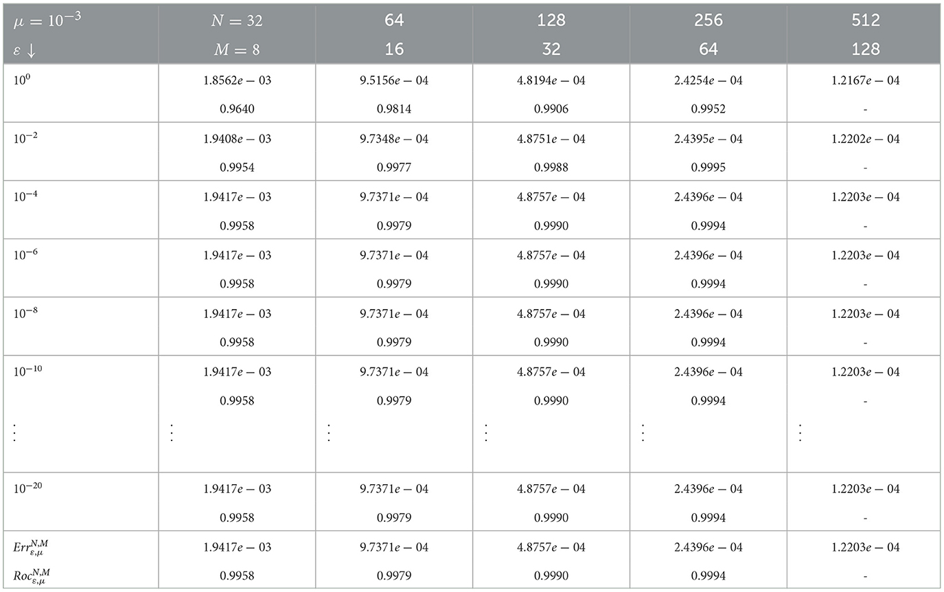
Table 1. Maximum errors $Er{r}_{\epsilon ,\mu }^{N,M}$ and rates of convergence $Ro{c}_{\epsilon ,\mu }^{N,M}$ using scheme (8) for example (5.1) with μ = 10⁻³ and different values of ε.

TABLE 2

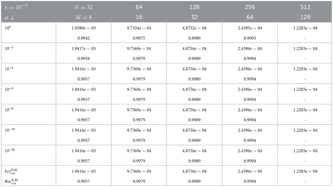
Table 2. Maximum errors $Er{r}_{\epsilon ,\mu }^{N,M}$ and rates of convergence $Ro{c}_{\epsilon ,\mu }^{N,M}$ using scheme (8) for example (5.1) with ε = 10⁻³ and different values of μ.

TABLE 3

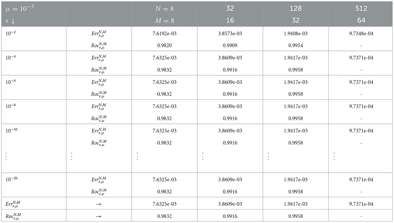
Table 3. Maximum errors $Er{r}_{\epsilon ,\mu }^{N,M}$ and rates of convergence $Ro{c}_{\epsilon ,\mu }^{N,M}$ using scheme (8) for example (5.1) with μ = 10⁻³ and different values of ε.

In Tables 4, 5, we computed the maximum pointwise errors and the corresponding rates of convergence for the numerical solution of example (5.1) using scheme (8). Thus, the results are presented by taking the values of μ and and ε as we have done for Tables 1, 2 and also using the discretization parameters N and M varying with the ratios of 2 and 4, respectively. Here, we show that the rate of convergence of the developed fitted operator finite difference scheme is almost two(confirm temporal order).

TABLE 4

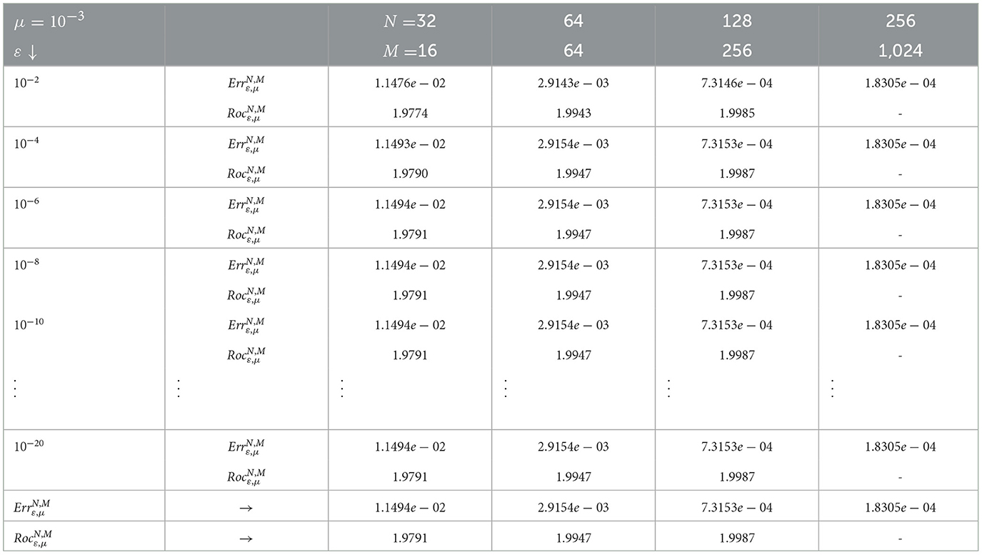
Table 4. Maximum errors $Er{r}_{\epsilon ,\mu }^{N,M}$ and rates of convergence $Ro{c}_{\epsilon ,\mu }^{N,M}$ using scheme (8) for example (5.1) with μ = 10⁻³ and different values of ε.

TABLE 5

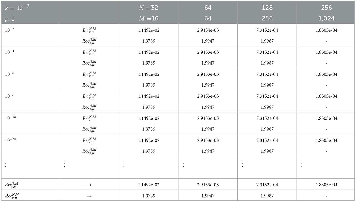
Table 5. Maximum errors $Er{r}_{\epsilon ,\mu }^{N,M}$ and rates of convergence $Ro{c}_{\epsilon ,\mu }^{N,M}$ using scheme (8) for example (5.1) with ε = 10⁻³ and different values of μ.

Table 6 shows the comparison of our scheme with the reference cited in Kumar and Kumar [44]. The comparison confirms that the maximum point-wise error, $Er{r}_{\epsilon ,\mu }^{N,M}$ obtained by our scheme is less than the error obtained by the scheme in Kumar and Kumar [44]. For the given example (5.1) the plotted Figures 1, 2 exhibit that the boundary layer behavior in the solution of the given problem. Again, the log-log plot in Figure 3 supports our theoretical error estimates.

TABLE 6

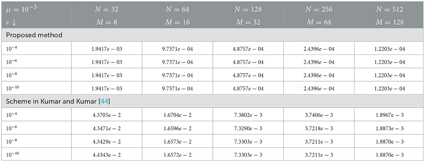
Table 6. Comparison of $Er{r}_{\epsilon ,\mu }^{N,M}$ of our scheme in (8) with an existing schemes in Kumar and Kumar [44] using example (5.1).

FIGURE 1

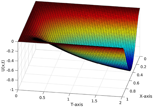
Figure 1. Numerical solution of example (5.1) for μ = 10⁻¹⁰ and ε = 10⁻³ taking N = 128 and M = 64.

FIGURE 2

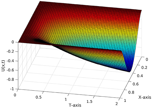
Figure 2. Numerical solution of example (5.1) for μ = 10⁻³ and ε = 10⁻¹⁰ taking N = 128 and M = 64.

FIGURE 3

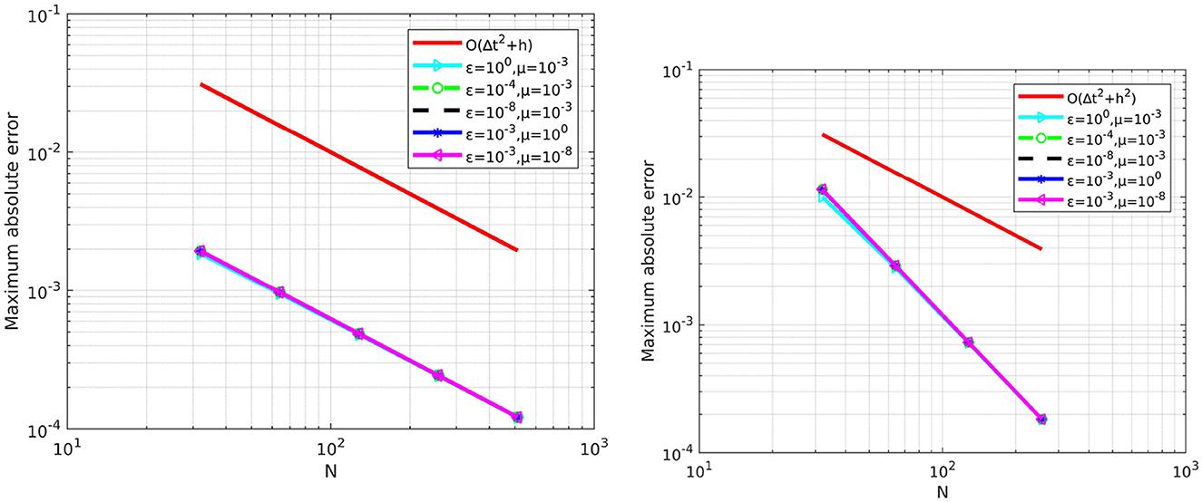
Figure 3. Log-Log plot N vs. maximum absolute errors for example (5.1).

6. Conclusion

We have developed a non-standard fitted operator finite difference method (NSFOFDM) for solving singularly perturbed time-delay partial differential equation with two perturbation parameters. In this study, uniform meshes have been considered in both space and time directions. The discretization was by using the implicit Crank-Nicolson finite difference method for time variable and a non-standard fitted operator finite difference(NSFOFDM) for space variable. The proposed numerical method is uniformly convergent independent of both the perturbation parameters, ε and μ. The scheme is shown to be first order in space and second order in time theoretically, but, we improved the order of convergence to the second order in both variables using temporal mesh refinement as shown in Tables 4, 5. To confirm the theoretical convergence results and to demonstrate the applicability of the proposed method, an example has been provided and results are presented in tables and graphs using Matlab software. The numerical example confirms the theoretical analyses. In our study, we considered two-parameter time-delay problem in one space dimensional. Future researches can be done in two space dimension.

Data availability statement

The original contributions presented in the study are included in the article/supplementary material, further inquiries can be directed to the corresponding author.

Author contributions

All authors contributed significantly, directly, and academically to the work and agreed to its publication.

Acknowledgments

The authors wish to acknowledge the referees for their constructive suggestions and comments.

Conflict of interest

The authors declare that the research was conducted in the absence of any commercial or financial relationships that could be construed as a potential conflict of interest.

Publisher's note

All claims expressed in this article are solely those of the authors and do not necessarily represent those of their affiliated organizations, or those of the publisher, the editors and the reviewers. Any product that may be evaluated in this article, or claim that may be made by its manufacturer, is not guaranteed or endorsed by the publisher.

References

1. Van Dyke M. Nineteenth-century roots of the boundary-layer idea. Siam Rev. (1994) 36:415–24. doi: 10.1137/1036097

CrossRef Full Text | Google Scholar

2. Prandtl L. Über Flussigkeitsbewegung bei sehr kleiner Reibung. Heidelberg: Verhandl III, Internat Math-Kong; Leipzig: Teubner (1904). p. 484–91.

Google Scholar

3. Chandru M, Das P, Ramos H. Numerical treatment of two-parameter singularly perturbed parabolic convection diffusion problems with non-smooth data. Math Methods Appl Sci. (2018) 41:5359–87. doi: 10.1002/mma.5067

CrossRef Full Text | Google Scholar

4. Zahra W, El Mhlawy AM. Numerical solution of two-parameter singularly perturbed boundary value problems via exponential spline. J King Saud Univ Sci. (2013) 25:201–8. doi: 10.1016/j.jksus.2013.01.003

CrossRef Full Text | Google Scholar

5. Abdelhakem M, Youssri Y. Two spectral Legendre's derivative algorithms for Lane-Emden, Bratu equations, and singular perturbed problems. Appl Num Math. (2021) 169:243–55. doi: 10.1016/j.apnum.2021.07.006

CrossRef Full Text | Google Scholar

6. Abd-Elhameed W, Youssri Y, Doha E. A novel operational matrix method based on shifted Legendre polynomials for solving second-order boundary value problems involving singular, singularly perturbed and Bratu-type equations. Math Sci. (2015) 9:93–102. doi: 10.1007/s40096-015-0155-8

CrossRef Full Text | Google Scholar

7. Polak S, Den Heijer C, Schilders W, Markowich P. Semiconductor device modelling from the numerical point of view. Int J Num Methods Eng. (1987) 24:763–838.

PubMed Abstract | Google Scholar

8. Chen J, O'Malley RE. Jr. On the asymptotic solution of a two-parameter boundary value problem of chemical reactor theory. SIAM J Appl Math. (1974) 26:717–29.

Google Scholar

9. Schlichting H, Kestin J. Boundary Layer Theory. Vol. 121. Berlin: Springer (1961).

Google Scholar

10. Friedrichs KO, Wasow WR. Singular perturbations of non-linear oscillations. Duke Math J. (1946) 13:367–81.

Google Scholar

11. Mickens RE. Nonstandard Finite Difference Models of Differential Equations. Singapore: World Scientific (1994).

Google Scholar

12. Kopteva N. Uniform pointwise convergence of difference schemes for convection-diffusion problems on layer-adapted meshes. Computing. (2001) 66:179–97. doi: 10.1007/s006070170034

CrossRef Full Text | Google Scholar

13. Roos HG, Uzelac Z. The SDFEM for a convection-diffusion problem with two small parameters. Comput Methods Appl Math. (2003) 3:443–58. doi: 10.2478/cmam-2003-0029

CrossRef Full Text | Google Scholar

14. Yüzbaşı Ş, Şahin N. Numerical solutions of singularly perturbed one-dimensional parabolic convection–diffusion problems by the Bessel collocation method. Appl Math Comput. Elsevier (2013) 220:305–15. doi: 10.1016/j.amc.2013.06.027

CrossRef Full Text | Google Scholar

15. Miller J, O'Riordan E, Shishkin G, Shishkina L. Fitted mesh methods for problems with parabolic boundary layers. In: Mathematical Proceedings of the Royal Irish Academy. JSTOR (1998). p. 173–90.

Google Scholar

16. O'Malley. Two-parameter singular perturbation problems for second-order equations. J Math Mech. (1967) 16:1143–64.

Google Scholar

17. O'Malley. Boundary value problems for linear systems of ordinary differential equations involving many small parameters. J Math Mech. (1969) 18:835–55.

Google Scholar

18. Munyakazi JB. A robust finite difference method for two-parameter parabolic convection-diffusion problems. Appl Math Inform Sci. (2015) 9:2877. doi: 10.12785/amis/090614

CrossRef Full Text | Google Scholar

19. Das P, Natesan S. Numerical solution of a system of singularly perturbed convection diffusion boundary value problems using mesh equidistribution technique. Aust J Math Anal Appl. (2013) 10:1–17.

Google Scholar

20. Das P. Comparison of a priori and a posteriori meshes for singularly perturbed nonlinear parameterized problems. J Comput Appl Math. (2015) 290:16–25. doi: 10.1016/j.cam.2015.04.034

CrossRef Full Text | Google Scholar

21. Das P, Natesan S. Higher-order parameter uniform convergent schemes for Robin type reaction-diffusion problems using adaptively generated grid. Int J Comput Methods. (2012) 9:1250052. doi: 10.1142/S0219876212500521

CrossRef Full Text | Google Scholar

22. Das P, Natesan S. Richardson extrapolation method for singularly perturbed convection-diffusion problems on adaptively generated mesh. Comput Model Eng Sci. (2013) 90:463–85.

Google Scholar

23. Das P, Natesan S. Adaptive mesh generation for singularly perturbed fourth-order ordinary differential equations. Int J Comput Math. (2015) 92:562–78. doi: 10.1080/00207160.2014.902054

CrossRef Full Text | Google Scholar

24. Dehghan M. Numerical solution of the three-dimensional advection–diffusion equation. Appl Math Comput. (2004) 150:5–19. doi: 10.1016/S0096-3003(03)00193-0

CrossRef Full Text | Google Scholar

25. Gracia J, O'Riordan E, Pickett M. A parameter robust second order numerical method for a singularly perturbed two-parameter problem. Appl Num Math. (2006) 56:962–80. doi: 10.1016/j.apnum.2005.08.002

CrossRef Full Text | Google Scholar

26. Kadalbajoo MK, Jha A. Exponentially fitted cubic spline for two-parameter singularly perturbed boundary value problems. Int J Comput Math. (2012) 89:836–50. doi: 10.1080/00207160.2012.663492

CrossRef Full Text | Google Scholar

27. Kaushik A. Singular perturbation analysis of bistable differential equation arising in the nerve pulse propagation. Nonlin Anal. (2008) 9:2106–27. doi: 10.1016/j.nonrwa.2007.06.014

CrossRef Full Text | Google Scholar

28. Kellogg RB, Tsan A. Analysis of some difference approximations for a singular perturbation problem without turning points. Math Comput. (1978) 32:1025–39.

Google Scholar

29. Linss T. A posteriori error estimation for a singularly perturbed problem with two small parameters. Int J Num Anal Model. (2010) 7:491–506.

Google Scholar

30. O'Riordan E, Pickett ML, Shishkin GI. Singularly perturbed problems modeling reaction-convection-diffusion processes. Comput Methods Appl Math. (2003) 3:424–42. doi: 10.2478/cmam-2003-0028

CrossRef Full Text | Google Scholar

31. Patidar KC. A robust fitted operator finite difference method for a two-parameter singular perturbation problem. J Diff Eq Appl. (2008) 14:1197–214. doi: 10.1080/10236190701817383

CrossRef Full Text | Google Scholar

32. Vulanović R. A higher-order scheme for quasilinear boundary value problems with two small parameters. Computing. (2001) 67:287–303. doi: 10.1007/s006070170002

CrossRef Full Text | Google Scholar

33. Chandru M, Prabha T, Shanthi V. A parameter robust higher order numerical method for singularly perturbed two parameter problems with non-smooth data. J Comput Appl Math. (2017) 309:11–27. doi: 10.1016/j.cam.2016.06.009

CrossRef Full Text | Google Scholar

34. Shanthi V, Ramanujam N, Natesan S. Fitted mesh method for singularly perturbed reaction-convection-diffusion problems with boundary and interior layers. J Appl Math Comput. (2006) 22:49–65. doi: 10.1007/BF02896460

CrossRef Full Text | Google Scholar

35. Bashier EB, Patidar KC. A novel fitted operator finite difference method for a singularly perturbed delay parabolic partial differential equation. Appl Math Comput. (2011) 217:4728–39. doi: 10.1016/j.amc.2010.11.028

CrossRef Full Text | Google Scholar

36. Kaushik A, Sharma K, Sharma M. A parameter uniform difference scheme for parabolic partial differential equation with a retarded argument. Appl Math Model. (2010) 34:4232–42. doi: 10.1016/j.apm.2010.04.020

CrossRef Full Text | Google Scholar

37. Kumar S, Kumar M. High order parameter-uniform discretization for singularly perturbed parabolic partial differential equations with time delay. Comput Math Appl. (2014) 68:1355–67. doi: 10.1016/j.camwa.2014.09.004

CrossRef Full Text | Google Scholar

38. Erdogan F, Cen Z. A uniformly almost second order convergent numerical method for singularly perturbed delay differential equations. J Comput Appl Math. (2018) 333:382–94. doi: 10.1016/j.cam.2017.11.017

CrossRef Full Text | Google Scholar

39. Cen Z. A second-order finite difference scheme for a class of singularly perturbed delay differential equations. Int J Comput Math. (2010) 87:173–85. doi: 10.1080/00207160801989875

CrossRef Full Text | Google Scholar

40. Singh J, Kumar S, Kumar M. A domain decomposition method for solving singularly perturbed parabolic reaction-diffusion problems with time delay. Num Methods Part Diff Eq. (2018) 34:1849–66. doi: 10.1002/num.22256

CrossRef Full Text | Google Scholar

41. Ansari A, Bakr S, Shishkin G. A parameter-robust finite difference method for singularly perturbed delay parabolic partial differential equations. J Comput Appl Math. (2007) 205:552–66. doi: 10.1016/j.cam.2006.05.032

CrossRef Full Text | Google Scholar

42. Kumar S, Kumar M. A second order uniformly convergent numerical scheme for parameterized singularly perturbed delay differential problems. Num Algorit. (2017) 76:349–60. doi: 10.1007/s11075-016-0258-9

CrossRef Full Text | Google Scholar

43. Govindarao L, Sahu SR, Mohapatra J. Uniformly convergent numerical method for singularly perturbed time delay parabolic problem with two small parameters. Iran J Sci Technol Trans A. (2019) 43:2373–83. doi: 10.1007/s40995-019-00697-2

CrossRef Full Text | Google Scholar

44. Kumar S, Kumar M. A robust numerical method for a two-parameter singularly perturbed time delay parabolic problem. Comput Appl Math. (2020) 39:1–25. doi: 10.1007/s40314-020-01236-1

CrossRef Full Text | Google Scholar

45. O'Riordan E, Pickett M, Shishkin G. Parameter-uniform finite difference schemes for singularly perturbed parabolic diffusion-convection-reaction problems. Math Comput. (2006) 75:1135–54. doi: 10.1090/S0025-5718-06-01846-1

CrossRef Full Text | Google Scholar

46. Kadalbajoo M, Yadaw AS. Parameter-uniform finite element method for two-parameter singularly perturbed parabolic reaction-diffusion problems. Int J Comput Methods. (2012) 9:1250047. doi: 10.1142/S0219876212500478

CrossRef Full Text | Google Scholar

47. Miller JJ, O'riordan E, Shishkin GI. Fitted Numerical Methods for Singular Perturbation Problems: Error Estimates in the Maximum Norm for Linear Problems in One and Two Dimensions. Singapore: World Scientific (1996).

Google Scholar

48. Doolan EP, Miller JJ, Schilders WH. Uniform Numerical Methods for Problems With Initial and Boundary Layers. Dublin: Boole Press (1980).

PubMed Abstract | Google Scholar