Log-Kumaraswamy distribution: its features and applications

1. Introduction

Modeling and analyzing natural phenomena are essential parts of statistical research in a broad variety of practical domains, including science and engineering. Over the past 3 decades, extensive studies have been conducted to introduce statistical models that can better capture the characteristics of natural phenomena [1]. Kumaraswamy established the two-parameter Kumaraswamy distribution for modeling data concerning hydrology [2]. This distribution has been used in many real-world scenarios with outcomes that have considerable limits, such as hydrological data, weights of persons, exam marks, the growth rate of species, wind speed, atmospheric temperature, medicine, physics, and financial data [3–5]. Despite its significance, the distribution did not attract much more attention in the statistical literature. However, Jones studied various features of the Kumaraswamy distribution, including the quantile function, L-moments, and order statistics [6]. The study found that this distribution has some properties in common with the beta distribution [7].

Recent developments in the Kumaraswamy distribution have [8] determined the generalized-order statistics from the Kumaraswamy model, [9] developed Bayesian and non-Bayesian estimators based on type II censored data, which described the shape parameters, reliability, and failure rate functions of this model, [10] obtained modified point estimators for Kumaraswamy model, [3] compared and evaluated the performance of 10 various approaches of estimation the parameters of a two-parameter Kumaraswamy model using Monte Carlo simulations, and [11] studied and derived the classical and Bayes estimation for the Kumaraswamy inverse exponential distribution.

Moreover, several new families of probability distributions have been introduced for modeling data in hydrology, medical science, engineering, insurance, and finance based on the Kumaraswamy distribution method, for instance, Kumaraswamy Weibull [12], Kumaraswamy generalized gamma [13], Kumaraswamy inverse Weibull [14], Kumaraswamy modified inverse Weibull [14], F-Weibull [15], Kumaraswamy Gumbel [16], Kumaraswamy log-logistic [17], Kumaraswamy exponentiated Pareto [18], Kumaraswamy modified Weibull [19], Kumaraswamy generalized Lomax [20], Kumaraswamy [21], Kumaraswamy half-Cauchy [22], Kumaraswamy generalized Rayleigh [23], Kumaraswamy skew-normal [24], Kumaraswamy inverse Weibull Poisson [25], odd beta prime-logistic distribution [26], Kumaraswamy Marshall-Olkin Fréchet [27], Kumaraswamy inverse flexible Weibull [28], Maxwell-exponential distribution [29], Kumaraswamy Laplace [30], extensions of the Gompertz and inverse Gaussian, Kumaraswamy Gompertz and Kumaraswamy inverse Gaussian distributions under the Kumaraswamy family of distributions [31], Kumaraswamy skew-t distribution [32], Kumaraswamy transmuted Pareto distribution [33], Kumaraswamy Marshall-Olkin log-logistic distribution [34], Kumaraswamy exponentiated Fréchet distribution [35], Kumaraswamy log-logistic Weibull distribution [36], Kumaraswamy alpha power inverted exponential distribution [37], Kumaraswamy Marshall-Olkin exponential distribution [38], odd beta prime Fréchet distribution [39], Kumaraswamy Inverted Topp–Leone distribution [40], log-Topp-Leone distribution [41], Kumaraswamy Harris generalized Kumaraswamy distribution [42], and generalized transmuted-Kumaraswamy distribution [43]. As studied in [44], Kumaraswamy's cumulative distribution function (cdf) with shape parameters α, β > 0 is given as

$\begin{array}{ll}F\left(y;\alpha ,\beta \right)=1-{\left(1-y^{\alpha }\right)}^{\beta },0<y<1& (1)\end{array}$

The corresponding probability density function (pdf) is

$\begin{array}{ll}f\left(y;\alpha ,\beta \right)=\alpha \beta y^{\alpha -1}{\left(1-y^{\alpha }\right)}^{\beta -1},0<y<1& (2)\end{array}$

This study extends the applicability and flexibility of the classical Kumaraswamy model so that it can be used to model bounded and unbounded real-life data sets. This can be achieved based on the following motivations:

i. To introduce a new flexible statistical distribution that serves as an alternative to bounded Kumaraswamy and some other distributions.

ii. To obtain a distribution with different densities and hazard shapes.

iii. To derive some important properties such as moments, information-generating function, and order statistics.

iv. To obtain its parameters using the maximum likelihood, least squares, maximum product of spacings, and weighted least squares methods of estimations.

v. To identify the performances and potentiality of the proposed distribution against other comparative ones by means of application to a real data set.

This study can be constituted as follows: Section 2 provides the pdf, cdf, survival, hazard, mixture representations, and quantile function of the log-Kumaraswamy distribution. Some statistical features of the proposed distribution including moments, information-generating function, and order statistics are studied in Section 3. Its parameters can be derived using the maximum likelihood given in Section 4. The maximum product of spacings, least squares, and weighted least squares methods of estimation can be obtained from the simulation study, and a real-life data set can be used to ascertain the performances and flexibility of the new distribution presented in Section 5. The study concluded in Section 6.

2. Log-Kumaraswamy distribution

The log-Kumaraswamy distribution is introduced in this section by transforming x = −log(1 − y) from the Kumaraswamy model given in (2) as

$\begin{array}{l}f\left(x;\alpha ,\beta \right)=\alpha \beta e^{-x}{\left(1-e^{-x}\right)}^{\alpha -1}\\ {\left(1-{\left(1-e^{-x}\right)}^{\alpha }\right)}^{\beta -1}\alpha ,\beta >0;x>0& (3)\end{array}$

In this regard, the parameters α, β denote shape as well. The corresponding cdf is acquired from (3) as

$\begin{array}{ll}F\left(x;\alpha ,\beta \right)=1-{\left(1-{\left(1-e^{-x}\right)}^{\alpha }\right)}^{\beta },\alpha ,\beta >0;x>0& (4)\end{array}$

Hence, (3) and (4) are the cdf and pdf of the proposed log-Kumaraswamy distribution. For different parameter values, we can display the plots of the proposed distribution provided in Figure 1.

FIGURE 1

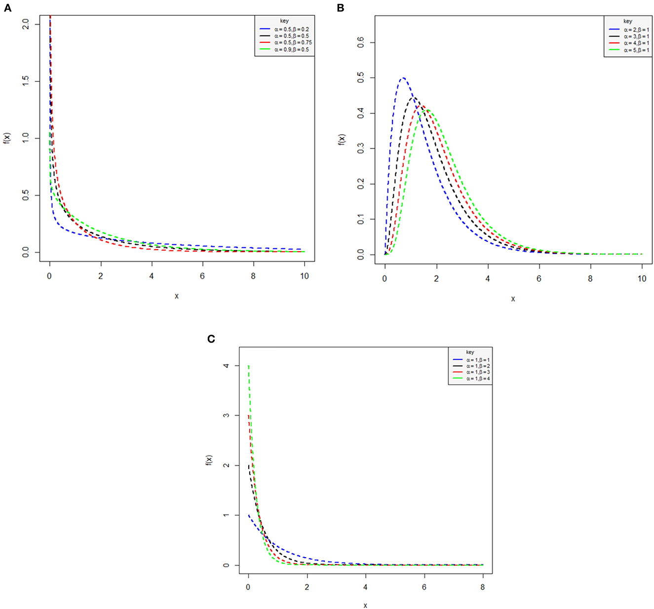
Figure 1. Pdf plots of the log-Kumaraswamy distribution using various set of values. Right-skewed function (A), right-skewed function (B), and right-skewed function (C).

It can be noticed from Figures 1A–C that for various parameter values of α and β, the log-Kumaraswamy's density shape provides a positive-skewed nature.

The survival and hazard functions are obtained by considering (3) and (4) as

$\begin{array}{ll}S\left(x;\alpha ,\beta \right)={\left(1-{\left(1-e^{-x}\right)}^{\alpha }\right)}^{\beta },\alpha ,\beta >0;x>0& (5)\end{array}$

and

$\begin{array}{ll}h\left(x;\alpha ,\beta \right)=\frac{\alpha \beta e^{-x}{\left(1-e^{-x}\right)}^{\alpha -1}}{1-{\left(1-e^{-x}\right)}^{\alpha }},\alpha ,\beta >0;x>0& (6)\end{array}$

It can be observed from (6) that for α = β = 1, ∀ x, then h(x; 1, 1) = 1. When β > 1 (say 2), then h(x; 1, 2) = 2, 3, 4, and so on. Similarly, keeping β = 1 and α > 1, then, h(x; α > 1, 1) = +ve.

The shapes of the hazard function can be determined numerically by applying Thomas's differential procedure [8] as

$\begin{array}{ll}\tau \left(x\right)=-\frac{f^{{}^{\prime }}\left(x\right)}{f\left(x\right)}.& (7)\end{array}$

where f′(x) is the first derivative of (3). For a differentiable probability density f(x) and hazard function h(x), one can obtain the first derivative of h(x) as

$\begin{array}{ll}{h}^{{}^{\prime }}\left(x\right)=h\left(x\right)\left\{h\left(x\right)-\tau \left(x\right)\right\}& (8)\end{array}$

Suppose h (x) > τ (x), ∀ x ∈ [L, U], where L and U are the lower and upper support of the pdf, then the hazard function of the probability distribution proves to be monotonic increasing (MI) and monotonic decreasing (MD) if h (x) < τ (x), ∀ x ∈ [L, U]. Similarly, for h (x) = τ (x), ∀x ∈ [L, U], then the probability distribution has a constant (C) failure rate which states clearly that h′ (x) = 0. In this aspect, it proven that f′ (x) obtained as

$\begin{array}{ll}{f}^{{}^{\prime }}\left(x\right)=f\left(x\right)\left\{\frac{\left(\alpha -1\right)e^{-x}}{1-e^{-x}}-\frac{\left(\beta -1\right)e^{-x}{\left(1-e^{-x}\right)}^{\alpha -1}}{1-{\left(1-e^{-x}\right)}^{\alpha }}-1\right\}& (9)\end{array}$

This implies that

$\begin{array}{ll}\tau \left(x\right)=1+\frac{\left(\beta -1\right)e^{-x}{\left(1-e^{-x}\right)}^{\alpha -1}}{1-{\left(1-e^{-x}\right)}^{\alpha }}-\frac{\left(\alpha -1\right)e^{-x}}{1-e^{-x}}& (10)\end{array}$

Heading from (10) for α = β = 1, and for all value of x, then τ (x; 1, 1) = 1. Similarly, when β > 1 (say 2), the τ (x; 1, 2) = 2, 3, 4, and so on. Keeping β = 1 and α > 1, then τ (x; α > 1, 1) > 1. The numerical illustrations to determine the shapes of the hazard function of the log-Kumaraswamy distribution are provided in Table 1.

TABLE 1

Table 1. Results of the hazard function of log-Kumaraswamy distribution for various parameter values.

Tables 1–3 present the results and the conditions that warrant the behavior of the shapes of the hazard function of the proposed distribution as studied by [45]. Based on the conditions suggested by [45], the hazard shape could either be constant, monotonically increasing or decreasing functions.

TABLE 2

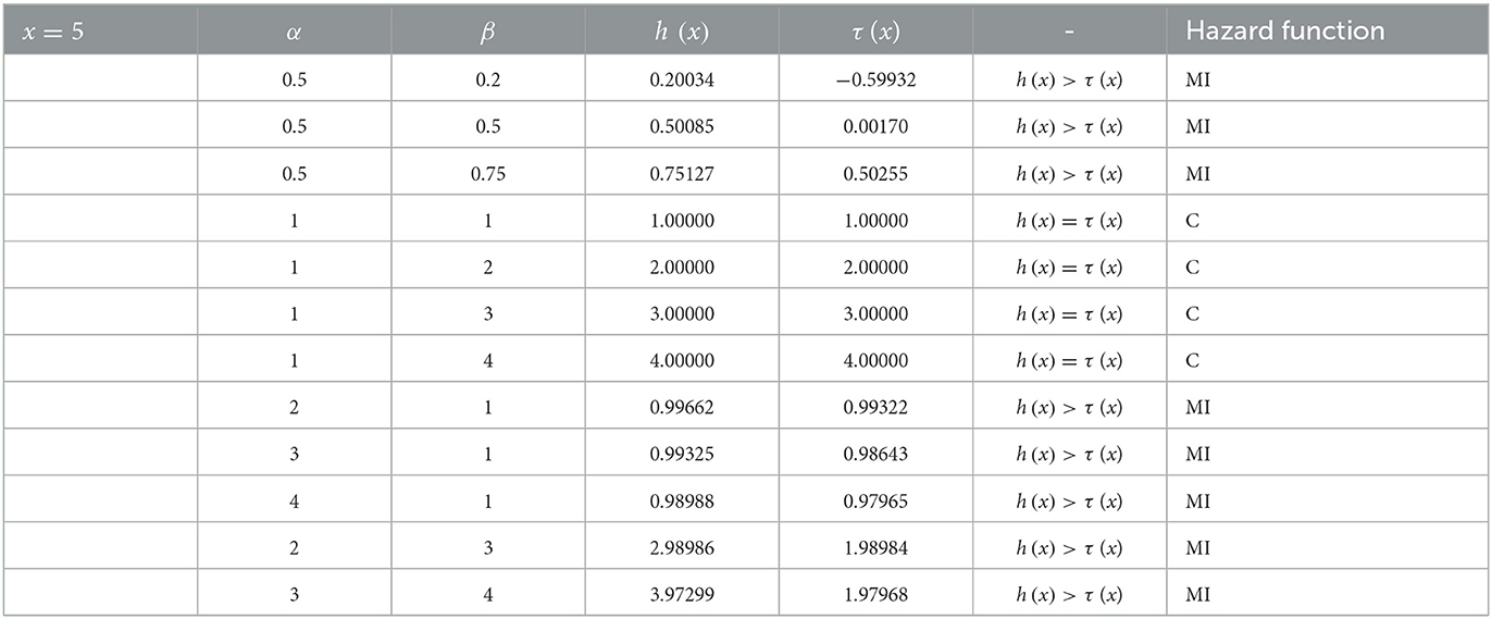
Table 2. Results of the hazard function of log-Kumaraswamy distribution for various parameter values.

TABLE 3

Table 3. Results of the hazard function of log-Kumaraswamy distribution for various parameter values.

It can be notable from Tables 1–3 that for α, β < 1, then h(x) > τ (x), this implies that the shape of the proposed distribution could be a monotonic increasing function. Keeping α = 1 and β ≥ 1, then h(x) = τ (x) and the hazard function is said to be a constant failure rate, and if α > 1, β = 1, or α > 1 and β > 1, then h(x) > τ (x) and the hazard function could also be a monotonically increasing function.

Plots of the hazard function by considering various parameter values that have been used in Tables 1–3 are provided in Figures 2A–D.

FIGURE 2

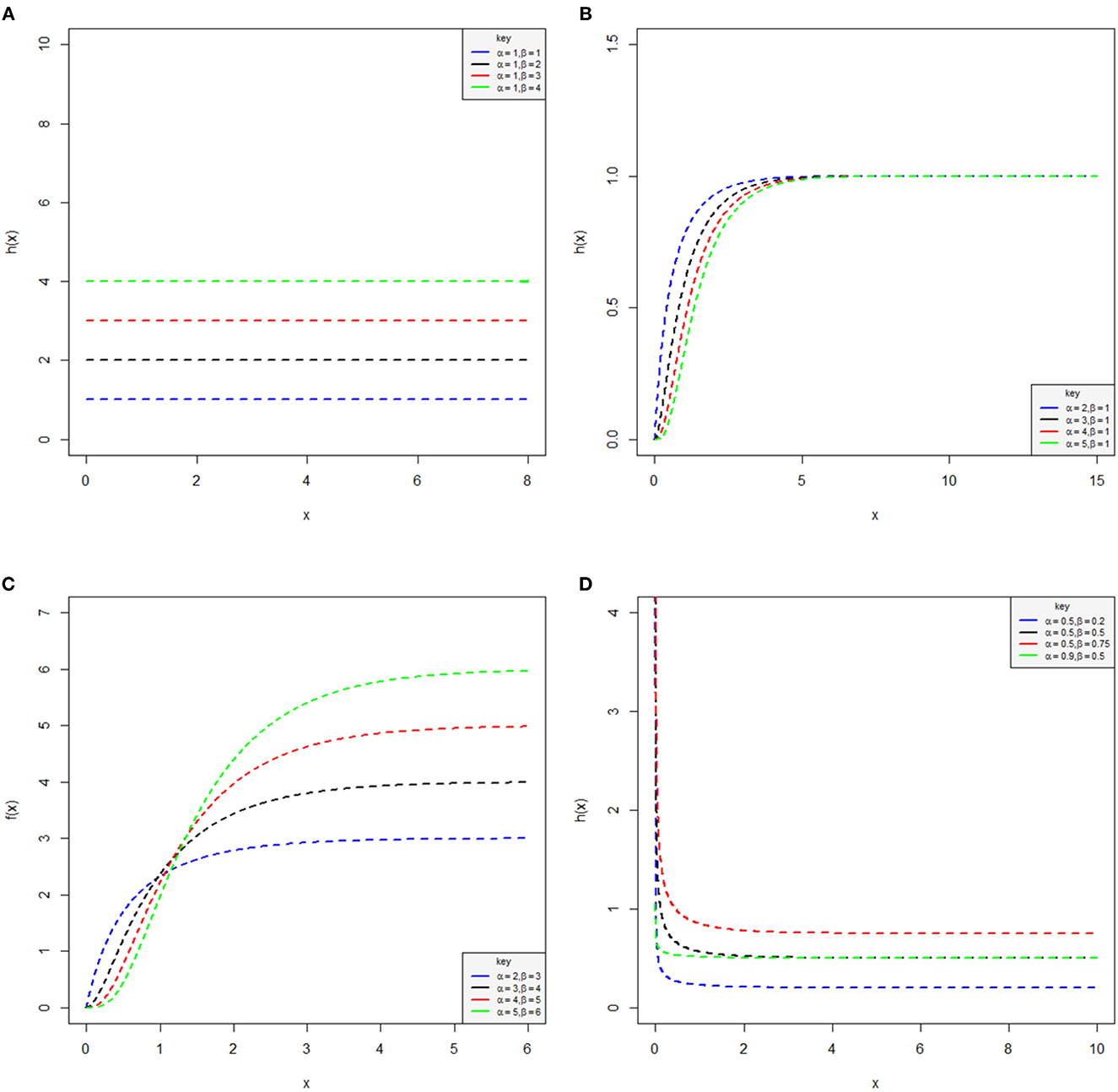
Figure 2. Plots of the hazard function of the log-Kumaraswamy distribution for various parameter values. Constant failure rate (A), monotonic increasing function (B), monotonic increasing function (C), and monotonic decreasing function (D).

Keeping α = 1 and β ≥ 1, the log-Kumaraswamy distribution has a constant failure rate, which is provided in Figure 2A. For α > 1 and β = 1 or α, β > 1, then the hazard function of the proposed distribution could be a monotonic increasing function presented in Figures 2B, C. It was observed from Figure 2D that for α, β < 1, the shape of the hazard function is a strictly monotonically decreasing function, which contradicts Tomas's theorem. Clearly, it is proven from these figures that the log-Kumaraswamy could be a constant, with monotonically increasing as well as decreasing failure rates.

2.1. Mixture representations

Consider the series expansion for |x| < 1 and τ > 0, then the expansion of this holds

$\begin{array}{ll}{\left(1-x\right)}^{\tau }={\displaystyle \sum _{j=0}^{\infty }}\frac{{\left(-1\right)}^j\Gamma \left(\tau +1\right)}{j!\Gamma \left(\tau -j+1\right)}{x}^j& (11)\end{array}$

Applying (11) into (3), it will become

$\begin{array}{ll}f\left(x\right)=\alpha \beta e^{-x}{\displaystyle \sum _{j=0}^{\infty }}\frac{{\left(-1\right)}^j\Gamma \left(\beta \right)}{j!\Gamma \left(\beta -j\right)}{\left(1-e^{-x}\right)}^{\alpha \left(1+j\right)-1}& (12)\end{array}$

We can express (12) by considering (11) as

$\begin{array}{ll}f\left(x\right)={\displaystyle \sum _{j,k=0}^{\infty }}{\varpi }_{j,k}{e}^{-x\left(1+k\right)}& (13)\end{array}$

which is the pdf of log-Kumaraswamy distribution expressed as mixture representations, where

$\begin{array}{l}{\varpi }_{j,k}=\frac{\alpha \beta {\left(-1\right)}^{j+k}\Gamma \left(\beta \right)\Gamma \left(\alpha \left(1+j\right)\right)}{j!k!\Gamma \left(\beta -j\right)\Gamma \left(\alpha \left(1+j\right)-k\right)}.\end{array}$

2.2. Quantile function

The quantile function of the log-Kumaraswamy distribution can be derived by inverting cdf in (4) as

$\begin{array}{ll}{\left(1-u\right)}^{1/\beta }=1-{\left(1-e^{-x}\right)}^{\alpha }& (14)\end{array}$

This can be expressed as

$\begin{array}{ll}{\left(1-{\left(1-u\right)}^{1/\beta }\right)}^{1/\alpha }=1-e^{-x}& (15)\end{array}$

which on simplification, gives the quantile function of the log-Kumaraswamy distribution as

$\begin{array}{ll}x=-ln\left\{1-{\left(1-{\left(1-u\right)}^{1/\beta }\right)}^{1/\alpha }\right\}:x_q& (16)\end{array}$

where u follows a uniform random variable on the interval (0, 1). The median of the log-Kumaraswamy distribution is obtained by setting

$\begin{array}{ll}u=0.5\text{as}{x}_m=-ln\left\{1-{\left(1-0.5^{1/\beta }\right)}^{1/\alpha }\right\}& (17)\end{array}$

3. Statistical features of the log-Kumaraswamy distribution

Some statistical features of log-Kumaraswamy distribution are provided in this section and include moments, information-generating function, and order statistics.

3.1. Moments

Suppose X is a random variable that follows log-Kumaraswamy distribution with pdf given in (13), then the moments of X are obtained as

$\begin{array}{ll}E\left(x^r\right)={\displaystyle \sum _{j,k=0}^{\infty }}{\bar{\omega }}_{j,k}{\displaystyle {\int }_0^{\infty }}{x}_r{e}^{-x\left(1+k\right)}dx& (18)\end{array}$

Let

$\begin{array}{ll}A=x\left(1+k\right),\Rightarrow dx=\frac{dA}{1+k}& (19)\end{array}$

Inserting (19) into (18) gives

$\begin{array}{l}E\left(x^r\right)=\frac{1}{{\left(1+k\right)}^{1+r}}{\displaystyle \sum _{j,k=0}^{\infty }}{\varpi }_{j,k}{\displaystyle {\int }_0^{\infty }}{A}^{\left(1+r\right)-1}{e}^{-A}dA\\ ={\displaystyle \sum _{j,k=0}^{\infty }}{\varpi }_{j,k}\frac{\Gamma \left(1+r\right)}{{\left(1+k\right)}^{1+r}}& (20)\end{array}$

which is the moments of log-Kumaraswamy distribution. Now, given r = 1, 2, then the mean and variance of the proposed distribution are, respectively, given as

$\begin{array}{ll}E\left(x\right)=\frac{1}{{\left(1+k\right)}^2}{\displaystyle \sum _{j,k=0}^{\infty }}{\varpi }_{j,k}& (21)\end{array}$

and

$\begin{array}{ll}V\left(x\right)=\frac{2}{{\left(1+k\right)}^3}{\displaystyle \sum _{j,k=0}^{\infty }}{\varpi }_{j,k}-{\left(\frac{1}{{\left(1+k\right)}^2}{\displaystyle \sum _{j,k=0}^{\infty }}{\varpi }_{j,k}\right)}^2& (22)\end{array}$

3.2. Information generating function

Let X follows log-Kumaraswamy distribution with pdf defined in (3). Then, the information generating function is defined as

$\begin{array}{ll}{I}_{\varphi }\left(x\right)={\displaystyle {\int }_{-\infty }^{\infty }}{f}^{\varphi }\left(x\right)dx& (23)\end{array}$

The integrand of (23) can be determined as

$\begin{array}{ll}{f}^{\varphi }\left(x\right)={\left(\alpha \beta \right)}^{\varphi }{e}^{-\varphi x}{\left(1-e^{-x}\right)}^{\varphi \left(\alpha -1\right)}{\left(1-{\left(1-e^{-x}\right)}^{\alpha }\right)}^{\varphi \left(\beta -1\right)}& (24)\end{array}$

Applying (11) into (24) gives

$\begin{array}{l}{f}^{\varphi }\left(x\right)={\left(\alpha \beta \right)}^{\varphi }{e}^{-phix}{\displaystyle \sum _{l=0}^{\infty }}\frac{{\left(-1\right)}^l\Gamma \left(\varphi \left(\beta -1\right)+1\right)}{l!\Gamma \left(\varphi \left(\beta -1\right)-l+1\right)}\\ {\left(1-e^{-x}\right)}^{\varphi \left(\alpha +1\right)+\alpha l}\\ ={\displaystyle \sum _{l,m=0}^{\infty }}{\text{Φ}}_{l,m}{e}^{-x\left(\varphi +m\right)}& (25)\end{array}$

where ${\text{Φ}}_{l,m}={\left(\alpha \beta \right)}^{\varphi }\frac{{\left(-1\right)}^{l+m}\Gamma \left(\varphi \left(\beta -1\right)+1\right)\Gamma \left(\varphi \left(\alpha -1\right)+\alpha l+1\right)}{l!m!\Gamma \left(\varphi \left(\beta -1\right)-l+1\right)\Gamma \left(\varphi \left(\alpha -1\right)+\alpha l-m+1\right)}$.

Substituting (35) into (23), it becomes

$\begin{array}{ll}{I}_{\varphi }\left(x\right)={\displaystyle \sum _{l,m=0}^{\infty }}{\text{Φ}}_{l,m}{\displaystyle {\int }_0^{\infty }}{e}^{-x\left(\varphi +m\right)}dx& (26)\end{array}$

Let

$\begin{array}{ll}y=x\left(\varphi +m\right),\Rightarrow dx=\frac{dy}{\varphi +m}& (27)\end{array}$

Putting (27) into (26) gives the information generating function of the log-Kumaraswamy distribution as

$\begin{array}{ll}{I}_{\varphi }\left(x\right)={\displaystyle \sum _{l,m=0}^{\infty }}\left(\frac{{\text{Φ}}_{l,m}}{\varphi +m}\right)& (28)\end{array}$

3.3. Renyi entropy

The Renyi entropy of log-Kumaraswamy distribution is defined as

$\begin{array}{ll}{R}_{\varphi }\left(x\right)=\frac{1}{1-\varphi }\left[{\displaystyle {\int }_{-\infty }^{\infty }}f{\left(x\right)}^{\varphi }dx\right],\varphi >0,\varphi \ne 1;x\in \Re & (29)\end{array}$

The integral in (29) has been obtained in (28). By substituting (28) into (29) gives the Renyi entropy of the proposed distribution as

$\begin{array}{ll}{R}_{\varphi }\left(x\right)=\frac{1}{1-\varphi }\left[{\displaystyle \sum _{l,m=0}^{\infty }}\left(\frac{{\text{Φ}}_{l,m}}{\varphi +m}\right)\right],\varphi >0,\varphi \ne 1& (30)\end{array}$

3.4. Q-entropy

The q-entropy of the log-Kumaraswamy distribution is obtained from (28) as

$\begin{array}{ll}{Q}_{\varphi }\left(x\right)=\frac{1}{\varphi -1}\left[1-{\displaystyle \sum _{l,m=0}^{\infty }}\left(\frac{{\text{Φ}}_{l,m}}{\varphi +m}\right)\right],\varphi \ne 1& (31)\end{array}$

3.5. Order statistics

Suppose X₁, X_{2, ...}, X_n denote the random variables which are independently and identically drawn from the sample sizes n with the pdf and cdf defined, respectively, in (3) and (4). The σ^th order statistics of those variables f_{σ, n}(x) is defined as

$\begin{array}{ll}{f}_{\sigma ,\kappa }\left(x\right)=\frac{\kappa !f\left(x\right)}{\left(\sigma -1\right)!\left(\kappa -\sigma \right)!}F{\left(x\right)}^{\sigma -1}{\left[1-F\left(x\right)\right]}^{\kappa -\sigma }& (32)\end{array}$

Substituting (3) and (4) into (32), one can obtain

$\begin{array}{ll}{f}_{\sigma ,\kappa }\left(x\right)={\displaystyle \sum _{l=0}^{\kappa -\sigma }}{\displaystyle \sum _{t=0}^{\infty }}{\text{Δ}}_{l,t}{e}^{-x}{\left(1-e^{-x}\right)}^{\alpha -1}{\left(1-{\left(1-e^{-x}\right)}^{\alpha }\right)}^{\beta \left(1+t\right)-1}& (33)\end{array}$

where ${\text{Δ}}_{l,t}=\frac{\alpha \beta \kappa !{\left(-1\right)}^{l+t}\Gamma \left(\sigma +l\right)\Gamma \left(\kappa -\sigma +1\right)}{\left(\sigma -1\right)!\left(\kappa -\sigma \right)!t!l!\Gamma \left(\sigma +l-t\right)\Gamma \left(\kappa -\sigma -l+1\right)}$.

Therefore, equation (33) can also be written by applying (11) as

$\begin{array}{ll}{f}_{\sigma ,\kappa }\left(x\right)={\displaystyle \sum _{l=0}^{\kappa -\sigma }}{\displaystyle \sum _{t,w,c=0}^{\infty }}{\text{Λ}}_{l,t,w,c}{e}^{-x\left(1+c\right)}& (34)\end{array}$

which is the σ^th order statistics of the log-Kumaraswamy distribution

where ${\text{Λ}}_{l,t,w,c}=\frac{{\text{Δ}}_{l,t}{\left(-1\right)}^{w+c}\Gamma \left(\beta \left(1+t\right)\right)\Gamma \left(\alpha \left(1+w\right)\right)}{w!c!\Gamma \left(\beta \left(1+t\right)-w\right)\Gamma \left(\alpha \left(1+w\right)-c\right)}$.

4. Parameter estimation

The parameters of the log-Kumaraswamy distribution will be obtained using maximum likelihood estimation (MLE) technique. Let X₁, X₂, ..., X_n denote the random sample drawn from the log-Kumaraswamy model with vector parameter Φ = α, β . The parameters of its estimates are derived by taking the likelihood function of (3) as

$\begin{array}{ll}\ell \left(x_i/\text{Φ}\right)={\left(\alpha \beta \right)}^n{e}^{-x_i}{\left(1-e^{-x_i}\right)}^{\alpha -1}{\left(1-{\left(1-e^{-x_i}\right)}^{\alpha }\right)}^{\beta -1},& (35)\end{array}$

The log-likelihood function of (35) denoted as L is given as

$\begin{array}{l}L=nlog\left(\alpha \right)+nlog\left(\beta \right)-{\displaystyle \sum _{i=1}^n}{x}_i+\left(\alpha -1\right){\displaystyle \sum _{i=1}^n}log\left(1-e^{-x_i}\right)\\ +\left(\beta -1\right){\displaystyle \sum _{i=1}^n}log\left(1-{\left(1-e^{-x_i}\right)}^{\alpha }\right)& (36)\end{array}$

We can now obtain the partial derivatives of (36) with respect to the parameters α and β as

$\begin{array}{l}\frac{\partial L}{\partial \alpha }=\frac{n}{\alpha }+{\displaystyle \sum _{i=1}^n}log\left(1-e^{-x_i}\right)-\left(\beta -1\right)\\ {\displaystyle \sum _{i=1}^n}\left(\frac{{\left(1-e^{-x_i}\right)}^{\alpha }log\left(1-e^{-x_i}\right)}{1-{\left(1-e^{-x_i}\right)}^{\alpha }}\right)& (37)\end{array}$

$\begin{array}{ll}\frac{\partial L}{\partial \beta }=\frac{n}{\beta }+{\displaystyle \sum _{i=1}^n}log\left(1-{\left(1-e^{-x_i}\right)}^{\alpha }\right)& (38)\end{array}$

Equating (37) and (38) to zero and simplifying for α and β gives the estimates of the parameters of the log-Kumaraswamy distribution. As observed, these estimates are non-linear and cannot be solved analytically, but with the aid of Matlab, R, Python, and more, we can obtain the estimators of $\widehat{\alpha }\mathrm{\text{ and }}\widehat{\beta }$.

5. Simulation study and data application

This section presents the simulation and real-life application of data sets.

5.1. Simulation study

In this section, we carried out a simulation study to assess the flexibility and performance of the estimators of parameters of the proposed distribution using different methods of estimation, including MLE, weighted least squares (WLS), least squares (LS), and maximum products of spacing (MPS). The simulation study was accomplished on the basis of the quantile function given in (16), and the data were generated from different sample sizes of n = 10, 20, 30, 50, 250, 500, and 1,000. The estimates of the vector parameter $\widehat{\text{Φ}}=\left(\widehat{\alpha },\widehat{\beta }\right)$ were obtained from the generated sample by maximizing the log-likelihood function given in (44). The simulation was repeated 1,000 times in which the mean estimates (mean) and mean square errors (MSE) were determined by setting Φ = (α, β) = (2, 1.5) and (3, 1.5), respectively, and the results of its estimates are well provided in Tables 4, 5.

TABLE 4

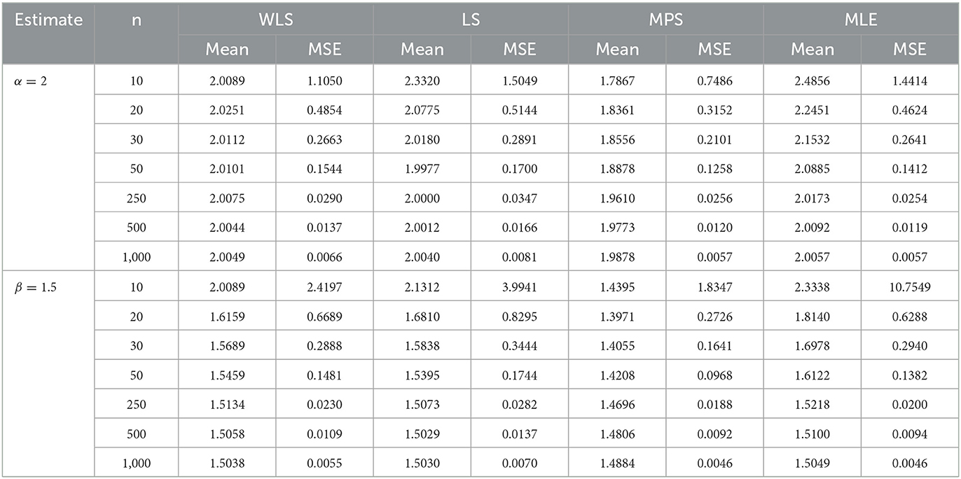
Table 4. Performance rating of the log-Kumaraswamy distribution using different methods of estimation.

TABLE 5

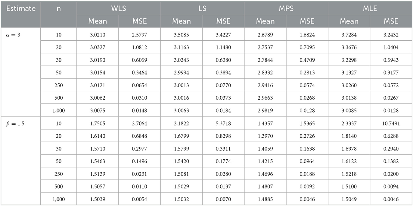
Table 5. Performance rating of the log-Kumaraswamy distribution using different methods of estimation.

Table 4 presents the estimates of the parameters using WLS, LS, MPS, and MLE methods with α = 2 and β = 1.5. As seen from Table 4, for the increasing sample sizes of n = 10, 20, 30, 50, 250, 500, and 1,000, the mean of each estimate using different methods of estimation approaches true parameter values. Similarly, the MSE of each estimate using different methods of estimation decreases, and hence, approaching zero. The table reveals that with increasing sample sizes, both MLE and MPS methods yield similar and superior results, producing lower MSE compared to WLS and LS methods, in that order. Table 5 provides the estimates of the parameters in which α = 3 and β = 1.5.

It can be revealed from Table 5 that the mean estimates of each parameter using the method of estimation approach fixed parameter values α = 3 and β = 1.5, respectively, as the sample size increases. The MSE of the parameters using the method of estimation decreases and converges to zero. It also proves that the MSE using MLE and MPS still approaches similar results as the sample size increases and hence provides the least MSE compared to other competing methods, followed by WLS and LS methods. This indicates from Tables 4, 5 that with the increase in sample sizes, the MSEs of MLE and MPS approached similar results and hence provided better estimates in comparison with WLS and LS as well.

5.2. Data application

An application to real-life data sets is presented in this section to ascertain the performance and potentiality of the log-Kumaraswamy model against its other competing distributions. The competing distributions used in this study are those with bounded and unbounded distributions such as Kumaraswamy, extended Kumaraswamy, Weibull, Gamma, Topp-Leone, log-normal, normal, and exponential distributions. We considered information criteria such as the Bayesian information criterion (BIC), Hannan–Quinn information criterion (HQIC), and consistent Akaike's information criterion (CAIC) as the statistical measure to check the best distribution among its competing ones, so the distribution with the least value of this measure will be selected as the one that best fits the data sets.

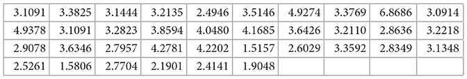
5.2.1. Data 1

The data set relates to the daily snowfall amounts of 30 observations measured in inches of water taken from non-seeded experimental units, which was conducted in the vicinity of Climax, Colorado [46]. The data are presented as follows:

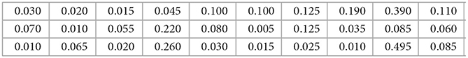
5.2.2. Data 2

An exchange rate data set related to a monthly Nigerian naira to CFA Francs consisting of 210 observations recorded from January 2004 to June 2021 was used and can be found in [47]. These data are presented as follows:

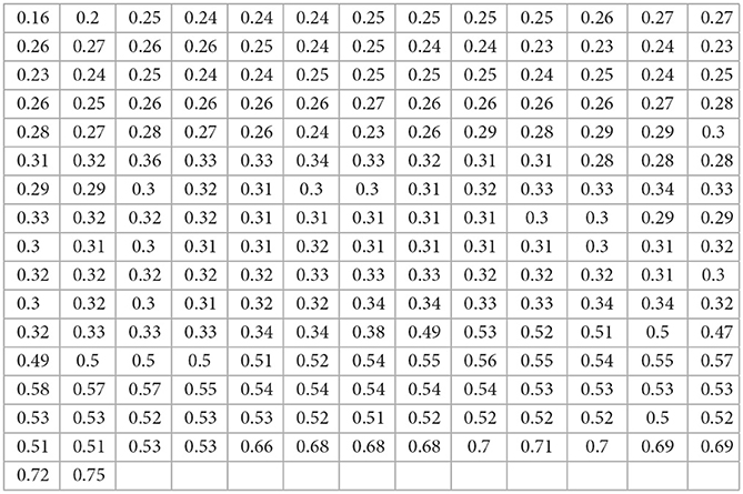
5.2.3. Data 3

The mortality rate data belonging to Canada of approximately 36 days reported from 10th April 2020 to 15th May 2020 were used to analyze the potentiality of the new distribution, see [48]. The data are presented as follows:

The summary of the data set, including mean, standard deviation, skewness, and kurtosis, is provided in Table 6. It can be observed from this table that the skewness of the data sets is positive and leptokurtic in nature since the computed kurtosis values are >3.

TABLE 6

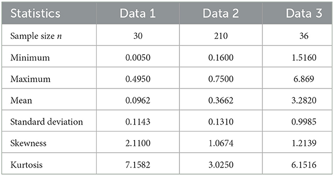
Table 6. Descriptive statistics for the data sets.

It is well known that the shape of the hazard function can be identified by appropriate total time on test (TTT) curves, as described in [49], and that if the curve is diagonally straight, the TTT has a constant failure function. For monotonically decreasing or increasing failure functions, then the TTT curves will be either concave or convex. Assume the failure rate is first convex and later concave; the TTT curve provides the bathtub; similarly, the curve is an appropriate unimodal failure rate. Figures 3A–C provides the TTT curves for the sets of data 1, 2, and 3, respectively.

FIGURE 3

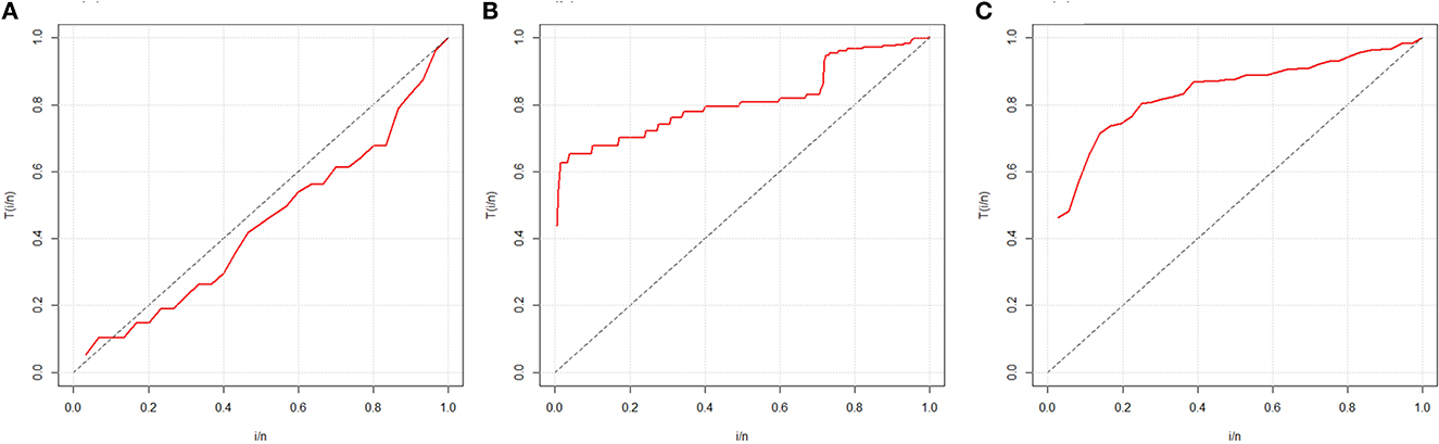
Figure 3. TTT curves for data 1 (A), 2 (B), and 3 (C).

It is shown from Figure 3A that the TTT curve for data 1 utilizes bathtub failure rate, while Figures 3B, C are indications of a monotonically increasing failure rate.

The density plots for the proposed log-Kumaraswamy distribution against its comparative distributions using data sets 1, 2, and 3 are provided in Figures 4A–C. It is shown from the figures that the log-Kumaraswamy distribution provides a reasonable fit irrespective of the other competing distributions.

FIGURE 4

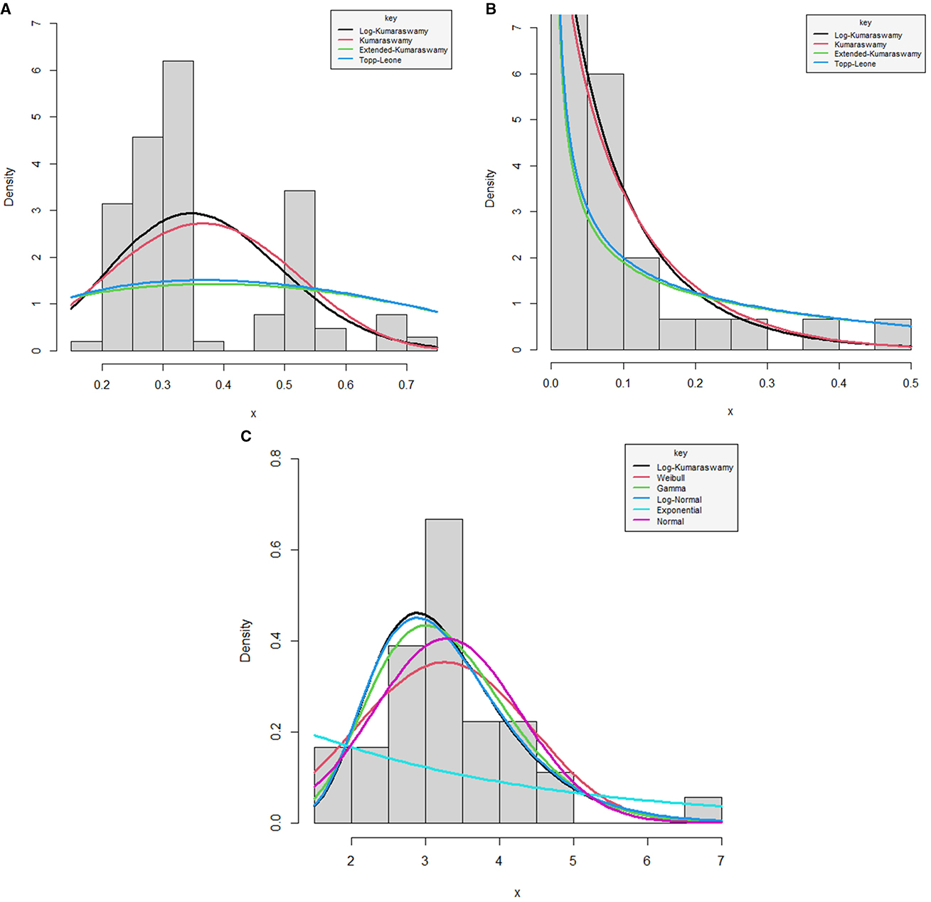
Figure 4. Fitted densities for the log-Kumaraswamy distribution and other competing models for data 1 (A), 2 (B), and 3 (C).

The performances for the log-Kumaraswamy distribution and other competing distributions with applications to real data sets 1, 2, and 3 are given in Tables 7–9, respectively, showing the estimates with their corresponding standard errors in parentheses, L, BIC, HQIC, and CAIC statistics.

TABLE 7

Table 7. Performance of the log-Kumaraswamy distribution against competing models using data 1.

The log-Kumaraswamy distribution gives the highest value of L and the least values of BIC, HQIC, and CAIC statistics compared to other comparative distributions, as presented in Tables 7, 8. This shows that the new distribution provided the best fit for the data sets relating to a daily snowfall and a monthly Nigerian naira to CFA Franc exchange rate. Table 9 presents the results of the log-Kumaraswamy distribution against unbounded models using data set 3.

TABLE 8

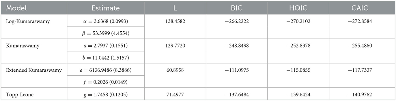
Table 8. Performances of the log-Kumaraswamy distribution against competing models using data 2.

TABLE 9

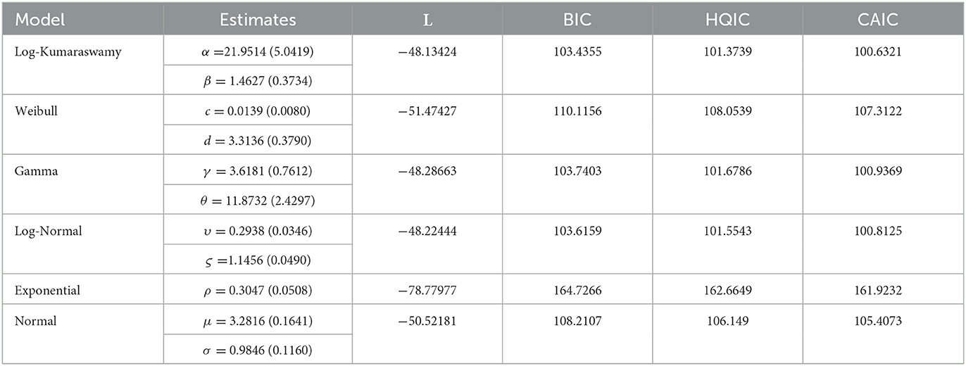
Table 9. Performance of the log-Kumaraswamy distribution against competing models using data 3.

It can be noticed from Table 9 that the new distribution provided the highest value of L and the least values of BIC, HQIC, and CAIC statistics compared other competing distributions. In this regard, the log-Kumaraswamy distribution could be a better choice for dealing with the bounded and unbounded distributions. This proved that the proposed distribution could accommodate positive real-life data sets.

6. Conclusion

This study developed a new extension of the classical Kumaraswamy distribution referred to as the log-Kumaraswamy distribution, which serves as a better alternative to some statistical distributions by means of applications to real-life data sets. It proves graphically and numerically that the density shapes could be skewed to the right and the hazard shape could either be a constant, monotonically decreasing, or increasing failure function. Some important features of this distribution are well identified, and the parameters of its estimates are obtained using MPS, MLE, LS, and WSL methods. We hope that the new distribution can be regarded as the best candidate for modeling data sets in a variety of practical fields, such as engineering, medical science, finance, hydrology, reliability, and insurance.

Data availability statement

The original contributions presented in the study are included in the article/supplementary material, further inquiries can be directed to the corresponding authors.

Author contributions

AI: Conceptualization, Methodology, Software, Writing—original draft. AS: Conceptualization, Methodology, Software, Writing—original draft, Writing—review & editing. HD: Conceptualization, Formal analysis, Funding acquisition, Investigation, Methodology, Project administration, Resources, Supervision, Validation, Visualization, Writing—review & editing. NS: Funding acquisition, Investigation, Validation, Visualization, Writing—review & editing. MO: Methodology, Supervision, Validation, Visualization, Writing—review & editing. RS: Funding acquisition, Investigation, Software, Supervision, Writing—review & editing. PW: Formal analysis, Investigation, Software, Visualization, Writing—review & editing. AU: Data curation, Software, Visualization, Writing—review & editing. SA: Writing—review & editing.

Funding

The author(s) declare financial support was received for the research, authorship, and/or publication of this article. This study was financially supported by the Yayasan Universiti Teknologi PETRONAS (YUTP) with the grant cost center 015LC0-401, INTI International University, Malaysia, and the National Collaborative Research Fund, Malaysia, with the grant cost center 015MCO-032.

Acknowledgments

The authors would like to thank Universiti Teknologi PETRONAS for providing support for this project. AS would also like to express his gratitude to Universiti Teknologi PETRONAS for sponsoring his Ph.D. studies and providing him with a position as a graduate assistant. The authors wish to extend their sincere thanks to the support of the Faculty of Data Science and Information Technology, INTI International University, Malaysia, for providing state-of-the-art research support to carry on this study. Finally, the authors express their gratitude to the referees for their insightful comments that improved the quality of this study.

Conflict of interest

The authors declare that the research was conducted in the absence of any commercial or financial relationships that could be construed as a potential conflict of interest.

Publisher's note

All claims expressed in this article are solely those of the authors and do not necessarily represent those of their affiliated organizations, or those of the publisher, the editors and the reviewers. Any product that may be evaluated in this article, or claim that may be made by its manufacturer, is not guaranteed or endorsed by the publisher.

References

1. Suleiman AA, Daud H, Singh NSS, Othman M, Ishaq AI, Sokkalingam R. The odd beta prime-G family of probability distributions: properties and applications to engineering and environmental data. Comp Sci Mathemat Forum. (2023) 7:20. doi: 10.3390/IOCMA2023-14429

CrossRef Full Text | Google Scholar

2. Kumaraswamy P. A generalized probability density function for double-bounded random processes. J Hydrol. (1980) 46:79–88. doi: 10.1016/0022-1694(80)90036-0

CrossRef Full Text | Google Scholar

3. Dey S, Mazucheli J, Nadarajah S. Kumaraswamy distribution: different methods of estimation. Comp Appl Mathemat. (2018) 37:2094–111. doi: 10.1007/s40314-017-0441-1

CrossRef Full Text | Google Scholar

4. Alshkaki R. A generalized modification of the Kumaraswamy distribution for modeling and analyzing real-life data. Stat Optim Inf Comput. (2020) 8:521–48. doi: 10.19139/soic-2310-5070-869

CrossRef Full Text | Google Scholar

5. Jamal F, Arslan Nasir M, Ozel G, Elgarhy M, Mamode Khan N. Generalized inverted Kumaraswamy generated family of distributions: theory and applications. J Appl Stat. (2019) 46:2927–44. doi: 10.1080/02664763.2019.1623867

CrossRef Full Text | Google Scholar

6. Jones M. Kumaraswamy's distribution: a beta-type distribution with some tractability advantages. Stat Methodol. (2009) 6:70–81. doi: 10.1016/j.stamet.2008.04.001

CrossRef Full Text | Google Scholar

7. Mahto AK, Lodhi C, Tripathi YM, Wang L. Inference for partially observed competing risks model for Kumaraswamy distribution under generalized progressive hybrid censoring. J Appl Stat. (2022) 49:2064–92. doi: 10.1080/02664763.2021.1889999

PubMed Abstract | CrossRef Full Text | Google Scholar

8. Garg M. On generalized order statistics from Kumaraswamy distribution. Tamsui Oxford J Inf Math Sci. (2009) 25:153–66.

Google Scholar

9. Gholizadeh R, Khalilpor M, Hadian M. Bayesian estimations in the Kumaraswamy distribution under progressively type II censoring data. Int J Eng Sci Technol. (2011) 3:47–65. doi: 10.4314/ijest.v3i9.4

CrossRef Full Text | Google Scholar

10. Lemonte AJ. Improved point estimation for the Kumaraswamy distribution. J Stat Comput Simul. (2011) 81:1971–82. doi: 10.1080/00949655.2010.511621

CrossRef Full Text | Google Scholar

11. Rastogi MK, Oguntunde PE. Classical and Bayes estimation of reliability characteristics of the Kumaraswamy-Inverse Exponential distribution. Int J Syst Assur Eng Manag. (2019) 10:190–200. doi: 10.1007/s13198-018-0744-7

CrossRef Full Text | Google Scholar

12. Cordeiro GM, Ortega EMM, Nadarajah S. The Kumaraswamy Weibull distribution with application to failure data. J Franklin Institute. (2010) 347:1399–429. doi: 10.1016/j.jfranklin.2010.06.010

CrossRef Full Text | Google Scholar

13. De Pascoa MA, Ortega EM, Cordeiro GM. The Kumaraswamy generalized gamma distribution with application in survival analysis. Statist Methodol. (2011) 8:411–33. doi: 10.1016/j.stamet.2011.04.001

CrossRef Full Text | Google Scholar

14. Shahbaz MQ, Shahbaz S, Butt NS. The Kumaraswamy-inverse weibull distribution. Pakistan J Stat Oper Res. (2012) 8:479–89. doi: 10.18187/pjsor.v8i3.520

CrossRef Full Text | Google Scholar

15. Ishaq AI, Usman A, Tasi'u M, Suleiman AA, Ahmad AG. A new odd F-Weibull distribution: properties and application of the monthly Nigerian naira to British pound exchange rate data. In: 2022 International Conference on Data Analytics for Business and Industry (ICDABI). Sakhir: IEEE (2022). p. 326–332.

Google Scholar

16. Cordeiro GM, Nadarajah S, Ortega EMM. The Kumaraswamy Gumbel distribution. Statist Meth Appl. (2012) 21:139–68. doi: 10.1007/s10260-011-0183-y

CrossRef Full Text | Google Scholar

17. De Santana TVF, Ortega EM, Cordeiro GM, Silva GO. The Kumaraswamy-log-logistic distribution. J Stat Theory Appl. (2012) 11:265–91.

Google Scholar

18. Elbatal I. The Kumaraswamy exponentiated pareto distribution. Econ Qual Control. (2013) 28:1–8. doi: 10.1515/eqc-2013-0006

CrossRef Full Text | Google Scholar

19. Cordeiro GM, Ortega EMM, Silva GO. The Kumaraswamy modified Weibull distribution: theory and applications. J Stat Comput Simul. (2014) 84:1387–411. doi: 10.1080/00949655.2012.745125

CrossRef Full Text | Google Scholar

20. Shams TM. The kumaraswamy-generalized lomax distribution. Middle East J Sci Res. (2013) 17:641–6.

Google Scholar

21. E-El-Sherpieny SA, Ahmed MA. On the Kumaraswamy distribution. Int J Basic Appl Sci. (2014) 3:372. doi: 10.14419/ijbas.v3i4.3182

CrossRef Full Text | Google Scholar

22. Indranil G. The Kumaraswamy-half-cauchy distribution: properties and applications. J Stat Theory Appl. (2014) 13:122–34. doi: 10.2991/jsta.2014.13.2.3

CrossRef Full Text | Google Scholar

23. Gomes AE, da-Silva CQ, Cordeiro GM, Ortega EMM. A new lifetime model: the Kumaraswamy generalized Rayleigh distribution. J Statist Comput Simul. (2014) 84:290–309. doi: 10.1080/00949655.2012.706813

CrossRef Full Text | Google Scholar

24. Mameli V. The Kumaraswamy skew-normal distribution. Statist Probab Lette. (2015) 104:75–81. doi: 10.1016/j.spl.2015.04.031

CrossRef Full Text | Google Scholar

25. Bera WT. The Kumaraswamy Inverse Weibull Poisson Distribution with Applications. Indiana: Indiana University of Pennsylvania (2015).

Google Scholar

26. Suleiman AA, Daud H, Singh NSS, Othman M, Ishaq AI, Sokkalingam R. A novel odd beta prime-logistic distribution: desirable mathematical properties and applications to engineering and environmental data. Sustainability. (2023) 15:10239. doi: 10.3390/su151310239

CrossRef Full Text | Google Scholar

27. Afify AZ, Yousof HM, Cordeiro GM, Nofal ZM, Ahmad M. The Kumaraswamy Marshall-Olkin Fréchet distribution with applications. J ISOSS. (2016) 2:151–68.

Google Scholar

28. Al Abbasi JN. Kumaraswamy inverse flexible Weibull distribution: theory and application. Int J Comp Applicat. (2016) 154:6. doi: 10.5120/ijca2016912223

CrossRef Full Text | Google Scholar

29. Abdullahi UA, Suleiman AA, Ishaq AI, Usman A, Suleiman A. The Maxwell–exponential distribution: theory and application to lifetime data. J Statist Model Analyt (JOSMA). (2021) 3:4. doi: 10.22452/josma.vol3no2.4

CrossRef Full Text | Google Scholar

30. Nassar MM. The Kumaraswamy laplace distribution. Pak J Stat Oper Res. (2016) 1485:609–24. doi: 10.18187/pjsor.v12i4.1485

CrossRef Full Text | Google Scholar

31. Rocha R, Nadarajah S, Tomazella V, Louzada F, Eudes A. New defective models based on the Kumaraswamy family of distributions with application to cancer data sets. Stat Methods Med Res. (2017) 26:1737–55. doi: 10.1177/0962280215587976

PubMed Abstract | CrossRef Full Text | Google Scholar

32. Said KK, Basalamah D, Ning W, Gupta A. The Kumaraswamy skew-t distribution and its related properties. Commun Stat - Simul Comput. (2018) 47:2409–23. doi: 10.1080/03610918.2017.1346801

CrossRef Full Text | Google Scholar

33. Chhetri SB, Akinsete AA, Aryal G, Long H. The Kumaraswamy transmuted Pareto distribution. J Stat Distrib Appl Ezoic. (2017) 4:11. doi: 10.1186/s40488-017-0065-4

CrossRef Full Text | Google Scholar

34. Selen C, Gamze O G. Yehia Mousa Hussein El, Hamedani GG. The Kumaraswamy Marshall-Olkin log-logistic distribution with application. J Stat Theory Appl.. (2018) 17:59–76. doi: 10.2991/jsta.2018.17.1.5

CrossRef Full Text | Google Scholar

35. Mansour MM, Aryal G, Afify AZ, Ahmad M. The Kumaraswamy exponentiated Fréchet distribution. Pak J Statist. (2018) 34:177–93.

Google Scholar

36. Mdlongwa P, Oluyede B, Amey A, Fagbamigbe A, Makubate B. Kumaraswamy log-logistic Weibull distribution: model, theory and application to lifetime and survival data. Heliyon. (2019) 5:e01144. doi: 10.1016/j.heliyon.2019.e01144

PubMed Abstract | CrossRef Full Text | Google Scholar

37. Thomas J, Zelibe SC, Eyefia E. Kumaraswamy alpha power inverted exponential distribution: properties and applications. Istatistik J Turkish Statist Associat. (2019) 12:35–48.

Google Scholar

38. George R, Thobias S. Kumaraswamy Marshall-Olkin exponential distribution. Commun Statistics-Theory Meth. (2019) 48:1920–37. doi: 10.1080/03610926.2018.1440594

CrossRef Full Text | Google Scholar

39. Suleiman AA, Daud H, Singh NSS, Othman M, Ishaq AI, Sokkalingam R, et al. Novel extension of the Fréchet distribution: statistical properties and application to groundwater pollutant concentrations. J Data Sci Insights. (2023) 1:8–24.

Google Scholar

40. Hassan AS, Almetwally EM, Ibrahim GM. Kumaraswamy inverted Topp–Leone distribution with applications to COVID-19 data. Comp Mater Continua. (2021) 2021:337–58. doi: 10.32604/cmc.2021.013971

CrossRef Full Text | Google Scholar

41. Usman A, Ishaq AI, Suleiman AA, Othman M, Daud H, Aliyu Y. Univariate and bivariate log-topp-leone distribution using censored and uncensored datasets. Comp Sci Mathemat Forum. (2023) 7:32. doi: 10.3390/IOCMA2023-14421

CrossRef Full Text | Google Scholar

42. Jisha V, Jose KK. Kumaraswamy Harris generalized Kumaraswamy distribution and its application in survival analysis. Biom Biostat Int J. (2022) 11:28–34.

Google Scholar

43. Ishaq AI, Usman A, Musa T, Agboola S. On some properties of Generalized Transmuted Kumaraswamy distribution. Pakistan J Statist Operat Res. (2019) 2019:577–86. doi: 10.18187/pjsor.v15i3.2344

CrossRef Full Text | Google Scholar

44. Sultana F, Tripathi YM, Rastogi MK, Wu S-J. Parameter estimation for the Kumaraswamy distribution based on hybrid censoring. Am J Mathemat Manage Sci. (2018) 37:243–61. doi: 10.1080/01966324.2017.1396943

CrossRef Full Text | Google Scholar

45. Thomas EA, Legge D. Probability matching as a basis for detection and recognition decisions. Psychol Rev. (1970) 77:65. doi: 10.1037/h0028579

CrossRef Full Text | Google Scholar

46. Mielke PW, Grant LO, Chappell CF. An independent replication of the Climax wintertime orographic cloud seeding experiment. J Appl Meteorol. (1962-1982). (1971) 1971:1198–1212.

Google Scholar

47. Ishaq A, Abiodun A, Panitanarak U. Modelling Nigerian Naira to CFA Franc Exchange Rates with Maxwell-Exponentiated Exponential distribution. In: 2021 International Conference on Data Analytics for Business and Industry (ICDABI). Sakheer: IEEE (2021). p. 342–347.

Google Scholar

48. Ishaq AI, Abiodun AA. On the developments of Maxwell-Dagum distribution. J Statist Model. (2021) 2:1–23.

Google Scholar

49. Aarset MV. How to identify a bathtub hazard rate. In: IEEE Transactions on Reliability. R-36. Sakheer: IEEE (1987). p. 106–108.

Google Scholar