Conditions for perfect transmission of quantum particles across layered heterostructures and resonance effects of an auxiliary well potential

We consider the bilayer heterostructure composed of the layer described by a rectangle-like potential and the background layer with an arbitrary potential profile given only by a transmission matrix. The conditions for the perfect (zero reflection) transmission of quantum particles across this structure is derived in the form of two basic equations on the rectangular layer parameters and the distance between the layers. The solution of these equations is analyzed in detail including some special cases and squeezing approximations. The effect of a rectangular well potential on the tunneling of particles with infinitesimally low energy through the background layer is investigated.

1 Introduction

In this paper, we derive some general conditions for resonant tunneling in the heterostructures composed of parallel layers. The electron motion in such a multi-layered structure is confined in the longitudinal direction (say, along the x-axis), which is perpendicular to the planes, and is free in the transverse direction. The three-dimensional Schrödinger equation of this structure can be separated into longitudinal and transverse parts, resulting in the reduced one-dimensional Schrödinger equation with respect to the longitudinal component of the wave function ψ(x) and the electron energy E. Thus, in the units as ℏ²/2m^* = 1, the one-dimensional stationary Schrödinger equation reads

$\begin{array}{ll}-{\psi }^{″}(x)+V(x)\psi (x)=E\psi (x),& (1)\end{array}$

where V(x) is a potential and the prime stands for the differentiation over the space x.

In general, resonant tunneling effects in heterostructures are studied when the potential profile V(x) is a compactly supported regular function. However, due to a rapid progress in fabricating micro- and nanodevices in recent years, the study of the electron transmission through heterostructures can additionally and effectively be investigated in the zero-thickness limit approximation when their width shrinks to zero. Within such an asymptotic approximation it is possible to produce the so-called point interaction models [see the book [1] for details and references], which are quite useful because they admit exact closed analytical solutions providing relatively simple situations, where an appropriate way of squeezing to zero can be chosen to be in relevance with a real structure. A whole body of literature [see, e.g., the works [2–11], to mention a few] has been published, where a number of interesting effects was discovered for the Schrödinger Equation 1 with the potentials in the form of distributions.

An example of such point interaction effects is the resonant tunneling through potentials squeezed to one point. This effect has been discovered and discussed in the works [12–23] for the potential V(x) = γδ′(x), δ′(x): = dδ(x)/dx, where δ(x) is Dirac's delta function and γ the potential strength. A non-zero transmission through this singular single-point potential (referred from now on to as the δ′-potential) has been shown to occur under certain conditions imposed on the strength γ, forming a discrete resonance set. It has been derived that the resonance set for the δ′-potential depends on the sequence of δ′-like regularizing functions. This leads to the conclusion about the existence of a hidden parameter in the Schrödinger Equation 1 with the δ′-potential.

The structures in which (regular) background potentials are perturbed by a point potential are also of significant importance. Thus, the perturbation of a harmonic oscillator by a so-called δ′-interaction [24] [the term adopted in the book [1] for which, at the point of singularity, the derivative ψ′(x) is continuous and ψ(x) discontinuous] as well as by a triple of δ′-interactions [25] has rigorously been defined as self-adjoint Hamiltonians. Another type of the point interactions, which were used as a perturbation of background potentials is the δ′-potential defined as the derivative of the delta function [the terms δ′-interaction and δ′-potential mean different point interactions, as suggested to distinguish these notions in Brasche and Nizhnik [26]]. This point interaction has been used as the perturbation of a constant electric field and a harmonic oscillator [27] as well as the perturbation of an infinite square well [28]. Three exactly solvable models with a one-dimensional V-shaped (conic) potential have been elaborated in the work [29]. These studies, which concern the perturbation of isotropic harmonic and conic potentials by a point interaction located at the origin have been extended to two and three dimensions in the papers [30–32]. All these systems are combined from a specific regular subsystem plus a point interaction centered inside this subsystem. In the work [33], the situation has been examined when a point interaction is found outside a background system at some finite distance.

In the present paper, we focus our attention on the perturbation of the background system with a general potential shape, which is characterized only by a transmission matrix. The perturbation is accomplished by a rectangle-like potential barrier/well located beyond the background system at an arbitrary distance. This potential geometry is applicable to heterostructures composed of two parallel layers described by corresponding potential profiles. A particular ubiquitous case of such systems is the double-barrier potential model that plays a key role in investigation of tunneling effects, beginning from the pioneering work [34, 35].

The motivation for this study is twofold. First, it is worthwhile to find the conditions for a perfect transmission across such a bilayer in the sense that there is no reflection of particles from the bilayer. Second, it would be of interest to investigate the effect of controlling the tunneling of particles with infinitesimally low energy through a background layer by “tuning” the parameters of an auxiliary rectangular well potential.

2 Preliminaries

Transmission matrix for a single layer structure: Consider a potential profile V(x) of an arbitrary shape with the support on the interval x₁ < x < x₂, where x₁ and x₂ are arbitrary points on the x-axis. The transmission matrix for Equation 1 that connects the boundary conditions at x = x₁ and x = x₂ is defined through the matrix equation

$\begin{array}{ll}\left(\begin{array}{c}\psi (x_2)\\ {\psi }^{\prime }(x_2)\end{array}\right)=\Lambda (\begin{array}{c}\psi (x_1)\\ {\psi }^{\prime }(x_1)\end{array}),\Lambda =\left(\begin{array}{c}{\lambda }_{11}{\lambda }_{12}\\ {\lambda }_{21}{\lambda }_{22}\end{array}\right),& (2)\end{array}$

where λ_ij ∈ ℝ and det Λ = 1.

For a structure consisting of one layer, it is supposed that V(x)≡h ∈ ℝ on some finite interval of length l and V(x)≡0 beyond this interval. When h>0 (h < 0), we are dealing with a barrier (a well), respectively. For this potential, the Λ-matrix (Equation 2) is calculated explicitly.

In the case when the potential V(x) in Equation 1 is a piecewise constant function, the Λ-matrix can be calculated explicitly. In particular, for the rectangle-like structure with the potential profile V(x) ≡ h ∈ ℝ defined on an interval x₁ < x < x₂ and V(x) ≡ 0 beyond this interval, the transmission matrix is

$\begin{array}{ll}\Lambda =\left(\begin{array}{c}cos(ql)q^{-1}sin(ql)\\ -qsin(ql)cos(ql)\end{array}\right),q:=\sqrt{k^2-h},l:=x_2-x_1.& (3)\end{array}$

Reflection-transmission probabilities expressed in terms of transmission matrix elements: For positive energy solutions of Equation 1 and the left-to-right current, let us define the reflection-transmission coefficients R and T through the scattering setting

$\begin{array}{ll}\psi (x;k)=\{\begin{array}{ll}{\text{e}}^{\text{i}kx}+R{\text{e}}^{-\text{i}kx}\hfill & \text{for }-\infty <x<x_1,\hfill \\ T{\text{e}}^{\text{i}kx}\hfill & \text{for }{x}_2<x<\infty ,\hfill \end{array}k:=\sqrt{E},E>0.& (4)\end{array}$

Using these expressions as boundary conditions at x = x₁ and x = x₂ in the matrix Equation 2, one can express the reflection and transmission probabilities in terms of the matrix elements λ_ij as follows

$\begin{array}{ll}R:=|R{|}^2=\frac{P^2+Q^2}{1+P^2+Q^2}\text{\hspace{1em}and\hspace{1em}}T:=|T{|}^2=\frac{1}{1+P^2+Q^2},& (5)\end{array}$

where

$\begin{array}{ll}P:=\frac{1}{2}({\lambda }_{11}-{\lambda }_{22})\text{and\hspace{1em}}Q:=\frac{1}{2}(k{\lambda }_{12}+k^{-1}{\lambda }_{21}).& (6)\end{array}$

Hence, according to Equations 5, 6, the transmission probability $T$ through the rectangular potential of height/depth h and width l reads

$\begin{array}{ll}T={\left[1+{\left(\frac{h}{2k}\right)}^2\frac{{\sin }^2(ql)}{k^2-h}\right]}^{-1},h\in ℝ,& (7)\end{array}$

where q is defined in Equation 3. As follows from this formula, no reflection occurs in the trivial case (h ≡ 0), i.e., $T$ = 1. The transmission of particles over the barrier/well with h ∈ ℝ\{0} is an oscillating function, while in the case of tunneling (k² ≤ h), the probability $T$ is a monotonically decreasing function of height h and width l.

Point interactions realized from rectangular potentials: In general, a point approximation of the Schrödinger Equation 1 can be implemented by replacing the potential V(x) by ε^−νV(x/ε), where ν>0 is an appropriate number and ε a dimensionless parameter that tends to zero, so that a given one-dimensional system (for instance, a layered heterostructure) shrinks to a point as ε → 0.

In the particular case of a rectangular barrier with height h>0 and thickness l, a point approximation is materialized by replacing realistic values of h and l by ε^−νh and εl, respectively. Inserting the replaced values into the transmission probability (Equation 7), for the tunneling through the barrier (k² ≤ h), we obtain

$\begin{array}{ll}T=\{\begin{array}{ll}1\hfill & \text{for }\nu <1,\hfill \\ {\left[1+{(\alpha /2k)}^2\right]}^{-1}\hfill & \text{for }\nu =1,\hfill \\ 0\hfill & \text{for }\nu >1,\hfill \end{array}\alpha :=hl.& (8)\end{array}$

It follows immediately from the comparison of the limit expressions (Equation 8) with the formula (Equation 7) that only the value ν = 1 turns out to be suitable for the point approximation of a rectangular barrier, whereas the values ν≠1 are not appropriate. The point interaction resulting from the approximation with ν = 1 is described by Dirac's delta function δ(x). It is called the δ-potential or δ-interaction. Its strength α is defined in Equation 8. The tunneling probability $T$ is a monotonically decreasing function of this strength and therefore this is an adequate description of the tunneling behavior. The corresponding Λ-matrix connecting the two-sided boundary conditions for the wave function ψ(x) and its derivative ψ′(x) at x = ±0, is obtained immediately as a ε → 0 limit of the matrix (Equation 3):

$\begin{array}{ll}\Lambda ={\Lambda }_{\delta }(\alpha ):=\left(\begin{array}{c}10\\ \alpha 1\end{array}\right).& (9)\end{array}$

The transmission probability across a well (k>0) with depth d>0 is determined by the same formula (Equation 7) where h is replaced by −d. In this case, instead of the monotonic behavior, the transmission $T$ is described by an oscillating function with the amplitude values $T$ = 1 at the points $\sqrt{k^2+d}l=n\pi$, n ∈ ℕ. Setting in Equation 7 h = −d, we obtain the non-trivial point limit of the transmission of particles over a squeezed rectangular well for two values of the parameter: ν = 1 and ν = 2. However, the value ν = 2 from the physical point of view is adequate and in this case we have

$\begin{array}{ll}T=T_{\vee }:=\{\begin{array}{ll}1\hfill & \text{for }\sqrt{d}l=n\pi ,\hfill \\ 0\hfill & \text{for }\sqrt{d}l\ne n\pi ,\hfill \end{array}n\in \mathbb{N}.& (10)\end{array}$

As follows from this asymptotic representation, only the value ν = 2 turns out to be closer to the realistic oscillating behavior described by Equation 7 where h = −d < 0. The value ν = 1 is not appropriate because the transmission $T$ for this value is a monotonically decreasing function. The other values ν and are not suitable because at these values the transmission is either perfect or completely reflective. However, unlike the barrier case, the non-zero transmission, being perfect, occurs only at some parameter values of the well forming a set of Lebesgue measure zero, namely

$\begin{array}{ll}{\Sigma }_{\vee }:=\left\{d,l|\sqrt{d}l=n\pi ,n\in \mathbb{N}\right\}.& (11)\end{array}$

This set consists of the countable family of curves on the {d, l}-plane. The transmission matrix is

$\begin{array}{ll}\Lambda ={\Lambda }_{\vee }:={(-1)}^{n}I,n\in \mathbb{N},& (12)\end{array}$

where I is the identity matrix.

3 A bilayer model

In the present paper, we consider a heterostructure composed of two parallel layers separated by a distance r>0, one of which (called A-layer) has a rectangular potential profile (barrier or well) and for the other one (called B-layer) the potential profile is of an arbitrary shape. More precisely, the potential in Equation 1 for this bilayer structure is defined by the function

$\begin{array}{ll}V(x)=\{\begin{array}{ll}h\in ℝ\setminus \left\{0\right\}\hfill & \text{for }{x}_1<x<y_1,\hfill \\ V_B(x)\hfill & \text{for }{x}_2<x<y_2,\hfill \\ 0\hfill & \text{otherwise},\hfill \end{array}& (13)\end{array}$

where y₁ < x₂ (so that r: = x₂ − y₁ > 0). Schematically, this potential profile is shown in Figure 1.

Figure 1

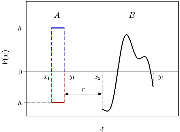
Figure 1. Potential setting for a bilayer structure. Both the potential profiles of the A-layer: the barrier of height h > 0 (blue) and the well of depth h < 0 (red) are shown in the form of rectangles.

The background B-layer is given by the transmission matrix that connects the boundary conditions at x = x₂ and x = y₂:

$\begin{array}{ll}C=\left(\begin{array}{c}{c}_{11}{c}_{12}\\ c_{21}{c}_{22}\end{array}\right),c_{ij}\in ℝ,detC=1.& (14)\end{array}$

Then the transmission matrix of the full bilayer system is the product Λ = CΛ₀ Λ _A, where the matrix Λ_A is given by Equation 3 with the A-layer parameters h and l, and the matrix

$\begin{array}{ll}{\Lambda }_0=\left(\begin{array}{c}cos(kr)k^{-1}sin(kr)\\ -ksin(kr)cos(kr)\end{array}\right)& (15)\end{array}$

corresponds to the free space between the layers. It is obtained from the Λ_A-matrix by setting there h = 0. As a result of computing the product, the elements of the full Λ-matrix become

$\begin{array}{ll}\begin{array}{c}{\lambda }_{11}=c_{11}\left[cos(ql)cos(kr)-(q/k)sin(ql)sin(kr)\right]\\ -c_{12}\left[kcos(ql)sin(kr)+qsin(ql)cos(kr)\right],\\ {\lambda }_{12}=c_{11}\left[k^{-1}cos(ql)sin(kr)+q^{-1}sin(ql)cos(kr)\right]\\ +c_{12}\left[cos(ql)cos(kr)-(k/q)sin(ql)sin(kr)\right],\\ {\lambda }_{21}=c_{21}\left[cos(ql)cos(kr)-(q/k)sin(ql)sin(kr)\right]\\ -c_{22}\left[kcos(ql)sin(kr)+qsin(ql)cos(kr)\right],\\ {\lambda }_{22}=c_{21}\left[k^{-1}cos(ql)sin(kr)+q^{-1}sin(ql)cos(kr)\right]\\ +c_{22}\left[cos(ql)cos(kr)-(k/q)sin(ql)sin(kr)\right].\end{array}& (16)\end{array}$

In the case if the A-layer is located behind the background layer, the transmission matrix is the product

$\begin{array}{ll}\bar{\Lambda }:={\Lambda }_A{\Lambda }_{0}C=\left(\begin{array}{c}{\bar{\lambda }}_{11}{\bar{\lambda }}_{12}\\ {\bar{\lambda }}_{21}{\bar{\lambda }}_{22}\end{array}\right).& (17)\end{array}$

The elements of this matrix are obtained from the matrix elements (Equation 16) by the following replacements:

$\begin{array}{ll}\begin{array}{c}{\bar{\lambda }}_{11}={\lambda }_{22}(c_{22}\to c_{11}),{\bar{\lambda }}_{12}={\lambda }_{12}(c_{11}\to c_{22}),\\ {\bar{\lambda }}_{21}={\lambda }_{21}(c_{22}\to c_{11}),{\bar{\lambda }}_{22}={\lambda }_{11}(c_{11}\to c_{22}).\end{array}& (18)\end{array}$

There is no loss of generality if we consider only the situation when the A-layer is located in front of the background layer. For this case, the conditions P = 0 and Q = 0 (see Equations 5, 6) for perfect transmission result in the following two equations:

$\begin{array}{l}u=\left[(q/k)c_{11}-(k/q)c_{22}\right]tan(ql)tan(kr)\\ +(q{c}_{12}+q^{-1}{c}_{21})tan(ql)+vtan(kr),& (19)\end{array}$

$\begin{array}{l}v=\left[(k^2/q)c_{12}+(q/k^2)c_{21}\right]tan(ql)tan(kr)\\ +\left[(q/k)c_{22}-(k/q)c_{11}\right]tan(ql)-utan(kr),& (20)\end{array}$

where

$\begin{array}{ll}u:=c_{11}-c_{22}\text{and\hspace{1em}}v:=k{c}_{12}+k^{-1}{c}_{21}.& (21)\end{array}$

The conditions (Equations 19, 20) can be considered as equations with respect to the unknowns tan(ql) and tan(kr). Here, all the terms with tan(ql) are real independently whether q is real or imaginary. Notice also that the quantities u and v in general depend on k.

In the particular case when the B-layer is fully transparent, i.e., u = v = 0, then we have tan(ql) = 0. This means that the A-layer is also transparent. More precisely, tan(ql) = 0 if and only if u = v = 0 and the distance r in this case is arbitrary. To prove this, we insert c₁₁ = c₂₂ (u = 0) and $c_{21}=-k^2{c}_{12}$ (v = 0) into Equations 19, 20 and assuming that tan(ql)≠0, these equations become

$\begin{array}{ll}tan(kr)=-k{c}_{12}/c_{11}\text{and\hspace{1em}}tan(kr)=c_{11}/k{c}_{12},& (22)\end{array}$

respectively, which are contradictory. Therefore tan(ql) = 0. Vice versa, assuming in Equations 19, 20 tan(ql) = 0, we obtain the equations

$\begin{array}{ll}u=vtan(kr)\text{and\hspace{1em}}v=-utan(kr),& (23)\end{array}$

which can be satisfied only if u = v = 0.

In a general case if u² + v² ≠ 0, the solution of Equations 19, 20 with respect to sin(ql) [or cot(ql)] and tan(kr) reads

$\begin{array}{ll}sin(ql)=\pm \frac{kq}{h}\sqrt{u^2+v^2}\text{or\hspace{1em}}cot(ql)=\pm \sqrt{\frac{{(h/kq)}^2}{u^2+v^2}-1},& (24)\end{array}$

$\begin{array}{ll}tan(kr)=\frac{k{q}^{-1}{c}_{11}-k^{-1}q{c}_{22}+vcot(ql)}{k^2{q}^{-1}{c}_{12}+k^{-2}q{c}_{21}-ucot(ql)}.& (25)\end{array}$

If the A-layer is located behind the background layer, the elements c₁₁ and c₂₂ must be rearranged in these equations, so that in Equation 25 we have to accomplish the replacement c₂₂→c₁₁ and u → −u.

The representation (Equations 24, 25) determines the relation between the whole set of system parameters: (i) the height/depth h and the thickness l of the rectangle-like A-layer, (ii) the characteristics of the B-layer provided by the elements c_ij(k) of the C-matrix (Equation 14), and (iii) the distance r between the layers, at which a given energy E = k² is transmitted across this bilayer structure perfectly (with zero reflection). It is important that this representation allows us to express explicitly (at any fixed energy E = k²) the parameters l and r as functions of h and the matrix elements c_ij(k). Indeed, from Equation 24, the width l is found as a function l = l(k; h; c_ij). Using this dependence in Equation 25, we find the function r = r(k; h; c_ij) of the same parameters.

Now it remains to prove the validity of the right-hand sides of both Equations 24, 25. Consider first the regime of tunneling through the A-layer (k² ≤ h). In this case, from Equation 24, we explicitly find the thickness of the A-layer:

$\begin{array}{ll}l=\frac{1}{\kappa }\text{arcsinh}\left(\frac{k\kappa }{h}\sqrt{u^2+v^2}\right),\kappa :=\sqrt{h-k^2},& (26)\end{array}$

while the other parameter r is calculated from Equation 25 where

$\begin{array}{ll}q=\text{i}\kappa ,cot(ql)=-\text{i}coth(\kappa l),coth(\kappa l)=\sqrt{1+\frac{{(h/k\kappa )}^2}{u^2+v^2}}.& (27)\end{array}$

Thus, we arrive at the following conclusion: For the perfect (zero reflection) transmission of particles with a given finite energy E = k² across the whole bilayer structure, in the regime as the particles tunnel through the A-barrier potential with height h > 0 (k² ≤ h), there exists a non-empty set of the system parameters defined as follows: The height h and the matrix C = C(k) can be arbitrary, but thickness l is uniquely defined by the expression (Equation 26) and the series of distances r is calculated according to Equation 25 where cot(ql) is given by Equation 27.

In the special case k² = h, the κ → 0 limit of Equations 26, 27 yields expressions

$\begin{array}{ll}l=\frac{\sqrt{u^2+v^2}}{k},& (28)\end{array}$

$\begin{array}{ll}r=\frac{1}{k}arctan\left(\frac{c_{11}\sqrt{u^2+v^2}+v}{k{c}_{12}\sqrt{u^2+v^2}-u}\right).& (29)\end{array}$

The solution with q>0 (h may be negative) corresponds to the situation when a particle passes over the barrier or well of the A-layer. In this case, Equation 24 is well-defined only if

$\begin{array}{ll}\frac{{\chi }^2}{1-\chi }\ge u^2(k)+v^2(k),\chi :=\frac{h}{k^2},-\infty <\chi \le 1.& (30)\end{array}$

Solving this inequality, we find the two critical values of h:

$\begin{array}{ll}{h}_{\pm }(k)=\frac{k^2}{2}(u^2+v^2)\left(\pm \sqrt{1+\frac{4}{u^2+v^2}}-1\right)<k^2& (31)\end{array}$

that determine the intervals

$\begin{array}{ll}-\infty <h\le h_{-}<0\text{and\hspace{1em}}0<h_{+}\le h<k^2& (32)\end{array}$

on which the values for the height/depth h are admissible. Thus, one can conclude: Contrary to the tunneling regime through the A-layer, for the perfect transmission of particles with a given finite energy E = k² over the A-barrier potential with height h>0 (k²>h), the values of barrier height must be bounded from below (h≥h₊). In the case of the transmission over the A-well potential with depth h < 0, the values of well depth must be bounded from above (h ≤ h₋). The countable sets of thickness l and spacing r are calculated according to Equations 24, 25, respectively.

Schematically, the regions of admissible values of height/depth h ∈ ℝ\{0} for the perfect transmission of particles with a given energy E = k² across the whole bilayer structure are represented in Figure 2 in the form a “band structure.” Here, the band h₋ < h < h₊ is a forbidden region for the perfect transmission.

Figure 2

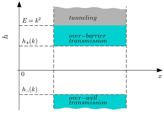
Figure 2. Regions of admissible values of height/depth h at which particles with a given energy E = k² are perfectly transmitted across the whole bilayer structure. Three regimes of transmission across the A-layer are shown by filled areas: tunneling (gray) and transmission over barrier and well (blue).

In the case as the background B-layer is completely transparent (i.e., u = v = 0), the A-layer must be also transparent. This can happen only in the case of a well (h = −d < 0) when $ql=\sqrt{E+d}l=n\pi$, n ∈ {0} ∪ ℕ. Therefore, the perfect transmission through the full system can be realized at the energies

$\begin{array}{ll}E=E_n={\left(\frac{n\pi }{l}\right)}^2-d\ge 0,n\ge \frac{\sqrt{d}l}{\pi },& (33)\end{array}$

and an arbitrary distance r > 0.

For the squeezed A-barrier, the δ-point approximation (h → ε⁻¹h and l → εl) with any strength α = hl reduces (Equations 24, 25) to

$\begin{array}{ll}\alpha =k\sqrt{u^2+v^2}& (34)\end{array}$

$\begin{array}{ll}tan(kr)=-\frac{v+c_{22}\sqrt{u^2+v^2}}{u+{\alpha }^{-1}{c}_{21}(u^2+v^2)}.& (35)\end{array}$

Therefore, for the perfect transmission through the full system, the strength α and the wave number k are coupled by Equation 34, and the distance r>0 is calculated from Equation 35.

For the A-well squeezed by the replacements d → ε⁻²d and l → εl (see also Equation 10), Equation 24 reduces to $tan(\sqrt{d}l)=0$, so that the A-well appears to be fully transparent only on the set $\sqrt{d}l=n\pi$, n ∈ ℕ. Therefore the perfect transmission across the full system can occur only if the background B-layer is also fully transparent, i.e., if u = v = 0. In this case, the distance r>0 is arbitrary.

4 Perfect transmission in the case of a rectangle-like B-layer

One of special cases of the perfect transmission through the bilayer structure is the trivial situation when one of the layers is fully transparent. Then the other layer must also be fully transparent. This is a trivial case when the layers do not interact and the distance between the layers is arbitrary.

The other cases when tan(ql)≠0 in Equation 24 and u² + v² ≠ 0 are non-trivial because of back and fourth reflections between the A- and B-layers. Below we will consider the cases when the elements of the C-matrix as well as the quantities u(k) and v(k) are given explicitly.

4.1 Rectangle-like potentials

In the particular case when the whole bilayer structure is composed of two rectangle-like layers, the quantities u(k) and v(k) can be calculated explicitly. Let us use here a symmetrized form of notations replacing h by h₁ and l by l₁. Denote the barrier/well parameters that describe the rectangular B-layer by h₂ and l₂, respectively. Thus, the whole system is assumed to be consisting of two rectangles, each of thickness l_j: = y_j − x_j and amplitude h_j ∈ ℝ\{0} (j = 1, 2), which are separated by distance r = x₂ − y₁ > 0. Denote also $q_j:=\sqrt{k^2-h_j}$. The origins h₁ = h₂ = 0 are excluded, otherwise the distance r does not make sense. In this case, we have

$\begin{array}{ll}u=0\text{and\hspace{1em}}v=\frac{h_2}{k{q}_2}sin(q_2{l}_2)& (36)\end{array}$

and therefore Equations 24, 25 can be represented in the form

$\begin{array}{l}\sin (q_1{l}_1)=\pm \frac{h_2{q}_1}{h_1{q}_2}\sin (q_2{l}_2)\text{\hspace{1em}or}\\ \cot (q_1{l}_1)=\pm \sqrt{{\left(\frac{h_1{q}_2}{h_2{q}_1}\right)}^2{\sin }^{-2}(q_2{l}_2)-1,}& (37)\end{array}$

$\begin{array}{l}tan(kr)=\frac{k}{(h_1+h_2)k^2-h_1{h}_2}\\ \left[q_1{h}_{2}cot(q_1{l}_1)+q_2{h}_{1}cot(q_2{l}_2)\right].& (38)\end{array}$

In the particular case of identical barriers (h₁ = h₂ ≡ h > 0, $q=\sqrt{k^2-h}$, k² ≤ h, l₁ = l₂ ≡ l), Equation 37 becomes an identity and Equation 38 reduces to the equation

$\begin{array}{ll}cot(kr)=\frac{1}{2}\left(\frac{k}{q}+\frac{q}{k}\right)tan(ql)& (39)\end{array}$

that describes the tunneling through the standard double-barrier system.

Since the C-matrix for the rectangle-like B-layer is given explicitly, the analytical results based on Equations 24, 25 can be verified numerically. One of the ways to solve this problem can be developed as follows. Based on the Equations 5, 6 for the transmission probability $T$, where the matrix elements λ_ij given by the expressions (Equation 16) and the transmission matrix for the B-layer

$\begin{array}{ll}C=\left(\begin{array}{c}cos(q_2{l}_2)q_2^{-1}sin(q_2{l}_2)\\ -q_{2}sin(q_2{l}_2)cos(q_2{l}_2)\end{array}\right)& (40)\end{array}$

are used, we compute the probability $T$ as a function of the wave number k fixing the system parameters. However, here the functional dependences l₁ = l₁(k; h₁; h₂, l₂) and r = r(k; h₁; h₂, l₂) described by Equations 37, 38 are inserted into the formulas for $T$ forming a “pathway” for the parameters l₁ and d. Then, fixing the parameters h₁, h₂ and l₂, we obtain the function $T$ = $T$(k). Therefore, if Equations 37, 38 correctly determine the parameter set {h₁, l₁; h₂, l₂; r}, at which a given energy E = k² is transmitted across the whole bilayer structure with zero reflection, then we have to get the identity $T$(k) ≡ 1 for all k>0. The numerical analysis has been accomplished for the three regimes: (i) the tunneling through the A-layer ($0<k^2<h_1$), (ii) the transmission over the A-barrier ($k^2>h_1$), and (iii) the transmission over the A-well, which correspond to the band structure illustrated by Figure 2. The results of this analysis are depicted in Figure 3, where it is demonstrated that $T$(k) ≡ 1 if both the dependences of l₁ and r on h₁, h₂ and l₂ are involved. It is illustrated that for some r lying beyond the pathway r = r(k; h₁, h₂, l₂), the identity $T$(k) ≡ 1 in general fails. The value $T$ = 1 reaches only at those r which appear on this pathway.

Figure 3

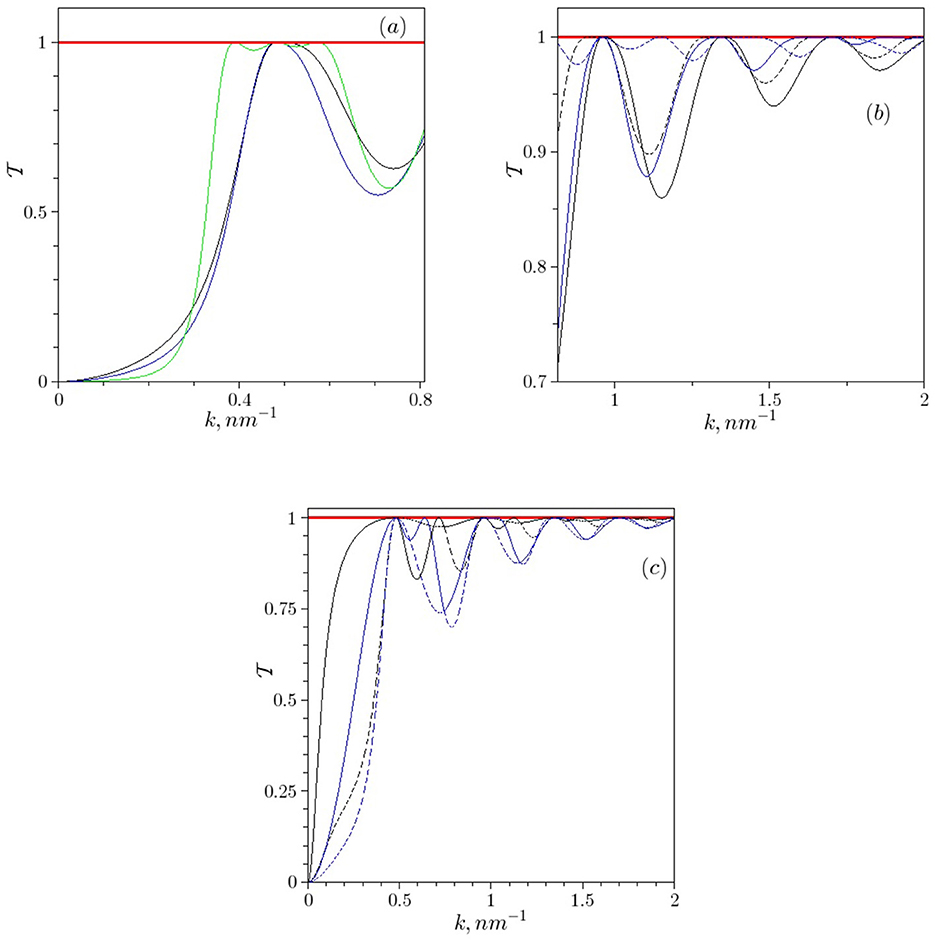
Figure 3. Transmission probability $T$ as a function of wave number k. The solid red straight lines $T$ ≡ 1 represent the calculations along the pathway defined by Equations 37, 38. Parameter values are h₁ = −h₂ = 0.25eV and l₂ = 10 nm. Calculations beyond the pathway (Equation 38), but for different fixed values of r, are represented by curves: (a) r = 0.25 nm (black), r = 1 nm (blue), r = 5 nm (green); (b, c) r = 0.25 nm (black), r = 1nm (blue). Here, the “+”-solutions are shown by solid lines and the “-”-solutions by dashed lines. The dimensions are chosen in the system for which ℏ²/2m^* = 1 where m^* is an effective electron mass. In the calculations we have set $m^{*}=0.1m_e$ where m_e is the free electron mass, so in our case 1 eV = 2.62464 nm⁻².

4.2 Point-like potentials

For realizing point interactions from rectangles in the bilayer structure we approximate a rectangle-like potential barrier for each layer by a δ-function (ν = 1) and a well by the squeezing rate with ν = 2 as described in Section 2. In other words, this approximation is suggested to be implemented by using the replacements: $h_j\to {\epsilon }^{-1}{h}_j$ (ν = 1, barrier), $d_j\equiv -h_j\to {\epsilon }^{-2}{d}_j$ (ν = 2, well) and l_j → εl_j (barrier and well), j = 1, 2.

First, we consider the case when only the B-layer is approximated by point potentials. In the case of a barrier (h₂ > 0), for its point approximation by a delta potential, we replace $h_2\to {\epsilon }^{-1}{h}_2$ and l₂ → εl₂. Then Equations 37, 38 reduce to

$\begin{array}{ll}sin(q_1{l}_1)=\pm \frac{q_1}{h_1}{\alpha }_2\text{or\hspace{1em}}cot(q_1{l}_1)=\pm \sqrt{{\left(\frac{h_1}{q_1{\alpha }_2}\right)}^2-1},& (41)\end{array}$

$\begin{array}{ll}tan(kr)=\frac{k}{q_1}\left[\frac{h_1}{{\alpha }_2{q}_1}+cot(q_1{l}_1)\right],& (42)\end{array}$

where h₁ ∈ ℝ\{0} and α₂: = h₂l₂ > 0 is a strength of the delta potential. These equations can be obtained directly from the basic Equations 19, 20, inserting there u = 0 and v = α₂/k. Similarly, when the A-layer is a α₁ δ (x) potential and the B-layer is a finite-thickness rectangle, in Equations 41, 42, the subscripts “1” and “2” have to be rearranged.

In the case of the point representation of the B-well, we replace in Equations 37, 38 $h_2\equiv -d_2\to -{\epsilon }^{-2}{d}_2$ and l₂ → εl₂. Then the only admissible case occurs if $\sqrt{d_2}{l}_2=n\pi$, n = 1, 2, …. It follows from Equation 37 that q₁ ≥ 0 and tan(q₁l₁) = 0 resulting in the condition $q_1{l}_1=\sqrt{k^2-h_1}{l}_1=m\pi$, m = 0, 1, …. Clearly, the distance r here is arbitrary.

Consider the case when both the A- and B-layers are point potentials. Here, the two-point squeezing can be defined by the limits x₁ → y₁ and y₂ → x₂ fixing the distance r. The only non-trivial case is that when both the layers are barriers. In this case, we obtain from Equation 37 that α₁ = α₂ ≡ α and from Equation 38 the equation

$\begin{array}{ll}tan(kr)=-2k/\alpha .& (43)\end{array}$

Note that this equation can also be obtained directly from Equation 39.

5 Effect of an auxiliary well on the tunneling of particles with extremely low energy

Consider a background B-layer structure described by the potential with an arbitrary shape. In particular, it may be a multi-layered structure. Assume that the transmission matrix C for the B-layer is defined by Equation 14, where the elements c_ij are arbitrary functions of the wave number k. Suppose also that the limits of c_ij(k)'s as k → 0, which describe the transmission of quantum particles with infinitesimally low energy, are finite. Then, as follows from the notations for u and v given in Equation 21, and the expression

$\begin{array}{ll}T=T_B=\frac{4}{4+u^2+v^2}& (44)\end{array}$

(see the second Equation 5), the zero-energy (k → 0) limit of tunneling through the B-layer is impossible if $\underset{k\to 0}{lim}{c}_{21}(k)\ne 0$.

Let us consider the k → 0 limit of the λ₂₁-element given in Equation 16 for the full system, where the A-layer is considered as an auxiliary well, also called a prewell [36]. Assume that the parameters of this well are characterized by depth d and width l. Setting $q=\sqrt{k^2+d}$ in λ₂₁, we obtain

$\begin{array}{ll}\frac{{\lambda }_{21}(k)}{k}~\left[cos(\sqrt{d}l)-r\sqrt{d}sin(\sqrt{d}l)\right]\frac{c_{21}(k)}{k}-\sqrt{d}\frac{sin(\sqrt{d}l)}{k}{c}_{22}(k).& (45)\end{array}$

Consider first the case when $\underset{k\to 0}{lim}{k}^{-1}{c}_{21}(k)$ is finite. In this case, $\underset{k\to 0}{lim}{c}_{22}\ne 0$ because detΛ = 1. The asymptotic equality (Equation 45) becomes finite if $sin(\sqrt{d}l)=0$. In the case if $\underset{k\to 0}{lim}{k}^{-1}{c}_{21}(k)$ is infinite, we need to provide the cancellation of divergences in Equation 45. Then $sin(\sqrt{d}l)\ne 0$ and therefore we get the equation

$\begin{array}{ll}\sqrt{d}tan\left(\sqrt{d}l\right)=\frac{1}{r+\rho },\rho :={\displaystyle \underset{k\to 0}{lim}}\frac{c_{22}(k)}{c_{21}(k)},& (46)\end{array}$

for the A-layer located in front of the background B-layer. In the other case as the A-layer is located behind the B-layer, the condition (Equation 46) has the same form where $\rho =\underset{k\to 0}{lim}(c_{11}/c_{21})$.

Thus, the presence of an auxiliary well (either in front of a background B-layer or behind it) provides a non-zero k → 0 limit of tunneling through the full system at some values of the parameters d and l being a solution of Equation 46. This solution forms the resonance set

$\begin{array}{ll}\Omega :=\left\{d,l|\sqrt{d}\text{ tan }(\sqrt{d}l)={(r+\rho )}^{-1}\right\}.& (47)\end{array}$

The set Ω includes the particular case as $\underset{k\to 0}{lim}{k}^{-1}{c}_{21}(k)$ is finite because in this case |ρ| → ∞, reducing Ω to the set

$\begin{array}{ll}\Omega =\left\{d,l|\sqrt{d}l=n\pi ,n\in \mathbb{N}\right\}.& (48)\end{array}$

6 Special cases of tunneling in the zero-energy limit

Consider the influence of an auxiliary rectangular well on single- and double-layer structures. In the case of barriers, the tunneling through these structures with infinitesimally low energy E = k² becomes impossible. However, as follows from Equation 46, a non-zero tunneling occurs at some values of the well parameters d and l that form the discrete set Ω defined by Equation 47.

6.1 Single-barrier structure

Let us consider as an example the case of a single background rectangular barrier. In this case, for such a barrier with height h_B and width l_B, according to Equation 3, the transmission C-matrix reads

$\begin{array}{ll}C=\left(\begin{array}{c}cosh({\kappa }_B{l}_B){\kappa }_B^{-1}sinh({\kappa }_B{l}_B)\\ {\kappa }_{B}sinh({\kappa }_B{l}_B)cosh({\kappa }_B{l}_B)\end{array}\right),{\kappa }_B:=\sqrt{h_B-k^2}.& (49)\end{array}$

Here, according to Equation 6,

$\begin{array}{ll}P=P_B=0\text{and\hspace{1em}}Q=Q_B=\frac{h_B}{2k{\kappa }_B}sinh({\kappa }_B{l}_B)& (50)\end{array}$

and, therefore, for the tunneling through the B-barrier alone (see the general second Equation 5) we obtain

$\begin{array}{ll}{T}_B={\left[1+\frac{{\sinh }^2({\kappa }_B{l}_B)}{4k^2{\kappa }_B^2}\right]}^{-1}\to 0& (51)\end{array}$

as k → 0. In the case when a pre-well is incorporated, for the probability $T$ of the whole bilayer structure, instead of the behavior (Equation 51), in the limit as k → 0, we get Q → 0, so that

$\begin{array}{ll}T=\frac{1}{1+P^2}& (52)\end{array}$

where

$\begin{array}{ll}{P}^2=\frac{1}{4}\left(\frac{d}{h_B}+\frac{h_B}{d}+2\right){sinh}^2(\sqrt{h_B}{l}_B){sin}^2(\sqrt{d}l).& (53)\end{array}$

In addition to this equation, in the k → 0 limit (see Equation 46), we have

$\begin{array}{ll}\rho =h_B^{-1/2}coth(\sqrt{h_B}{l}_B).& (54)\end{array}$

One can check numerically how the incorporation of a rectangular well provides the appearance of resonance peaks in the tunneling through the full system. To this end, we have performed the direct calculation of the transmission of low-energy particles through the full bilayer structure based on the Equations 5, 6, inserting the matrix elements c_ij(k) given by Equation 49 into the elements (Equation 16) where $q=\sqrt{k^2+d}$. As a result, the transmission probability $T$ is represented by a contour graph in Figure 4 as a function $T$ = $T$(d, l).

Figure 4

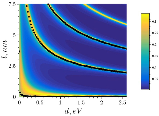
Figure 4. Transmission probability $T$ as a function of pre-well parameters d (depth) and l (width). Black curves (points) that represent the resonance set Ω given by Equation 47 are shown for the first three resonances with n = 1, 2, 3. Parameters of the background barrier are h_b = 0.1eV, l_B = 2 nm and r = 100 nm. The dimensions are chosen in the same system as for Figure 3.

6.2 Double-layer structure

In the following, we denote $C^0:=\underset{k\to 0}{lim}C(k)$. In the case of a double-layer system with heights h_j ∈ ℝ\{0}, j = 1, 2, using the k → 0 limit of the matrix elements (Equation 16), we obtain

$\begin{array}{r}\frac{C_B^0}{cos(\sqrt{-h_1}{l}_1)cos(\sqrt{-h_2}{l}_2)}\\ =\left(\begin{array}{c}1+h_2^{-1}{\tau }_1{\tau }_2-{\tau }_1{r}_0-h_1^{-1}{\tau }_1-h_2^{-1}{\tau }_2+r_0\\ -{\tau }_1-{\tau }_2+{\tau }_1{\tau }_2{r}_{0}1+h_1^{-1}{\tau }_1{\tau }_2-{\tau }_2{r}_0\end{array}\right)& (55)\end{array}$

where

$\begin{array}{ll}{\tau }_j:=\sqrt{-h_j}tan(\sqrt{-h_j}{l}_j),j=1,2,& (56)\end{array}$

and r₀ is a distance between the barriers. Here, the subscript B denotes the four possible configurations: B = bb (double-barrier), B = bw (barrier-well), B = wb (well-barrier), and B = ww (double-well).

Let Ω_B be a set of the parameter values for a given B-configuration at which the transmission of particles in the limit as k → 0 is possible. This behavior occurs if the c₂₁-element of the matrix (Equation 55) is zero. As a result, we obtain the following Ω_B-sets:

$\begin{array}{ll}\begin{array}{l}{\Omega }_{bb}=\varnothing ,\hfill \\ {\Omega }_{bw}=\left\{h_1,l_1;d_2,l_2;r|s_1^{-1}+t_2^{-1}=r_0\right\},\hfill \\ {\Omega }_{wb}=\left\{d_1,l_1;h_2,l_2;r|t_1^{-1}+s_2^{-1}=r_0\right\},\hfill \\ \text{}{\Omega }_{ww}=\left\{d_1,l_1;d_2,l_2;r|t_1^{-1}+t_2^{-1}=r_0\right\},\hfill \end{array}& (57)\end{array}$

where s_j: = −τ_j(h_j > 0) and t_j: = τ_j(h_j < 0). Therefore, for the B-configurations with a well, the k → 0 limiting transmission is possible even without the presence of an auxiliary well at the parameter values given in the sets (Equation 57). The “switching on” of the additional rectangular well with the parameters d and l given by the set (Equation 48) provides the transmission on the sets (Equation 57). However, beyond the set (Equation 48), the transmission on the sets (Equation 57) is impossible. Instead, it occurs on the sets (Equation 47), so that the sets (Equation 57) appear to be shifted accordingly. In other words, we have here the effect of controlling the transmission of zero-energy particles through a double-layer structure by “tuning” the parameters d and l of the auxiliary rectangular well.

In the case as the double-layer structure is approximated by two-point interactions, the k → 0 limit of the matrices C_B becomes

$\begin{array}{ll}\begin{array}{l}{C}_{\delta \delta }^0=\left(\begin{array}{l}1+{\alpha }_1{r}_0{r}_0\hfill \\ {\alpha }_1+{\alpha }_2+{\alpha }_1{\alpha }_2{r}_{0}1+{\alpha }_2{r}_0\hfill \end{array}\right),\hfill \\ C_{\delta \vee }^0={(-1)}^n\left(\begin{array}{c}1+{\alpha }_1{r}_0{r}_0\\ {\alpha }_{1}1\end{array}\right),\sqrt{d_2}{l}_2=n\pi ,\hfill \\ C_{\vee \delta }^0={(-1)}^n\left(\begin{array}{l}1r_0\hfill \\ {\alpha }_{2}1+{\alpha }_2{r}_0\hfill \end{array}\right),\sqrt{d_1}{l}_1=n\pi ,\hfill \\ C_{\vee \vee }^0={(-1)}^{m+n}\left(\begin{array}{l}1r_0\hfill \\ 01\hfill \end{array}\right),\sqrt{d_1}{l}_1=n\pi ,\sqrt{d_2}{l}_2=n\pi .\hfill \end{array}& (58)\end{array}$

Here, α_j > 0, so that only the double-well configuration admits the transmission of zero-energy particles. Notice that the connection matrices C_B with B = δ∨, ∨δ and ∨∨ make sense only under the conditions pointed out in Equation 58.

7 Concluding remarks

In summary, we have determined the two types of conditions, which are useful for the analysis of transmission across bilayer heterostructures. The potential profile of one (background) layer is assumed to have an arbitrary shape. It is only specified by a transmission matrix C with real elements for which detC = 1. The profile of the other layer is considered in the form of a rectangle, which may be either a barrier or a well.

The first type of conditions concerns the perfect (zero reflection) transmission across the bilayer structure. We have derived the system of two general Equations 24, 25 with respect to the parameters of the rectangular layer and the elements of the C-matrix. For a given energy E = k², height/depth h and the elements c_ij(k), one can explicitly calculate the A-layer thickness l from Equation 24 and then find the series of distances r using Equation 25. The only restriction on the A-layer parameters is that the well has to be sufficiently deep according to the inequalities (Equation 32).

The second type of conditions describes the general effect of the A-well on the transmission of particles with infinitesimally low energies E = k² across the whole bilayer structure with the B-layer of an arbitrary potential profile provided by the transmission C-matrix. Even in the case as the B-barrier is fully non-transparent for zero-energy particles, the presence of an auxiliary well always leads to a non-zero transparency of these particles at some parameter values of this well. A general Equation 46 for finding these resonant values has been derived. The particular cases where the transmission matrix C = C_B for the B-layer can be computed explicitly, have been considered. Here, these cases are specified by rectangular single- and double-layers. It is shown that in the case of barriers, a rectangular A-well makes the tunneling of zero-energy particles through these barrier structures possible on certain resonance sets. Notice that from the point of view of fabricating nanodevices, the transmission of quantum particles with extremely low energy in heterostructures is of big interest.

Data availability statement

The original contributions presented in the study are included in the article/supplementary material, further inquiries can be directed to the corresponding author.

Author contributions

YZ: Formal analysis, Visualization, Writing – original draft, Data curation, Writing – review & editing, Conceptualization, Validation, Investigation, Methodology. AZ: Validation, Conceptualization, Writing – review & editing, Methodology, Writing – original draft, Formal analysis, Investigation.

Funding

The author(s) declare that financial support was received for the research and/or publication of this article. The authors acknowledge the partial financial support from the National Academy of Sciences of Ukraine (YZ, Project No. 0122U000887 and AZ, Project No. 0122U000888).

Acknowledgments

We are indebted to the Referees for the careful reading of this paper, their questions and suggestions, resulting in the significant improvement of the paper. Finally, we also would like to thank the Armed Forces of Ukraine for providing security to perform this work.

Conflict of interest

The authors declare that the research was conducted in the absence of any commercial or financial relationships that could be construed as a potential conflict of interest.

Generative AI statement

The author(s) declare that no Gen AI was used in the creation of this manuscript.

Any alternative text (alt text) provided alongside figures in this article has been generated by Frontiers with the support of artificial intelligence and reasonable efforts have been made to ensure accuracy, including review by the authors wherever possible. If you identify any issues, please contact us.

Publisher's note

All claims expressed in this article are solely those of the authors and do not necessarily represent those of their affiliated organizations, or those of the publisher, the editors and the reviewers. Any product that may be evaluated in this article, or claim that may be made by its manufacturer, is not guaranteed or endorsed by the publisher.

References

1. Albeverio S, Gesztesy F, Hóegh-Krohn R, Holden H. Solvable Models in Quantum Mechanics. 2nd ed. With appendix by P. Exner. Providence, RI: AMS Chelsea (2005). doi: 10.1090/chel/350

Crossref Full Text | Google Scholar

2. Coutinho FAB, Nogami Y, Perez JF. Generalized point interactions in one-dimensional quantum mechanics. J Phys A Math Gen. (1997) 30:3937–45. doi: 10.1088/0305-4470/30/11/021

Crossref Full Text | Google Scholar

3. Albeverio S, Da̧browski L, Kurasov P. Symmetries of Schrödinger operators with point interactions. Lett Math Phys. (1998) 45:33–47. doi: 10.1023/A:1007493325970

Crossref Full Text | Google Scholar

4. Coutinho FAB, Nogami Y, Tomio L. Many-body system with a four-parameter family of point interactions in one dimension. J Phys A Math Gen. (1999) 32:4931–42. doi: 10.1088/0305-4470/32/26/311

Crossref Full Text | Google Scholar

5. Gadella M, Negro J, Nieto LM. Bound states and scattering coefficients of the −aδ(x)+bδ′(x) potential. Phys Lett A. (2009) 373:1310–3. doi: 10.1016/j.physleta.2009.02.025

Crossref Full Text | Google Scholar

6. Lunardi JT, Manzoni LA, Monteiro W. Remarks on point interactions in quantum mechanics. J Phys Conf Ser. (2013) 410:012072. doi: 10.1088/1742-6596/410/1/012072

Crossref Full Text | Google Scholar

7. Calçada M, Lunardi JT, Manzoni LA, Monteiro W. Distributional approach to point interactions in one-dimensional quantum mechanics. Front Phys. (2014) 2:23. doi: 10.3389/fphy.2014.00023

Crossref Full Text | Google Scholar

8. Lange RJ. Distribution theory for Schrödinger's integral equation. J Math Phys. (2015) 56:122105. doi: 10.1063/1.4936302

Crossref Full Text | Google Scholar

9. Konno K, Nagasawa T, Takahashi R. Effects of two successive parity-invariant point interactions on one-dimensional quantum transmission: resonance conditions for the parameter space. Ann Phys. (2016) 375:91–104. doi: 10.1016/j.aop.2016.09.012

Crossref Full Text | Google Scholar

10. Konno K, Nagasawa T, Takahashi R. Resonant transmission in one-dimensional quantum mechanics with two independent point interactions: full parameter analysis. Ann Phys. (2017) 385:729–43. doi: 10.1016/j.aop.2017.08.031

Crossref Full Text | Google Scholar

11. Erman F, Turgut OT. A perturbative approach to the tunneling phenomena. Front Phys. (2019) 7:69. doi: 10.3389/fphy.2019.00069

PubMed Abstract | Crossref Full Text | Google Scholar

12. Christiansen PL, Arnbak NC, Zolotaryuk AV, Ermakov VN, Gaididei YB. On the existence of resonances in the transmission probability for interactions arising from derivatives of Dirac's delta function. J Phys A Math Gen. (2003) 36:7589–600. doi: 10.1088/0305-4470/36/27/311

Crossref Full Text | Google Scholar

13. Zolotaryuk AV, Christiansen PL, Iermakova SV. Scattering properties of point dipole interactions. J Phys A Math Gen. (2006) 39:9329–38. doi: 10.1088/0305-4470/39/29/023

Crossref Full Text | Google Scholar

14. Toyama FM, Nogami Y. Transmission-reflection problem with a potential of the form of the derivative of the delta function. J Phys A Math Theor. (2007) 40:F685–90. doi: 10.1088/1751-8113/40/29/F05

Crossref Full Text | Google Scholar

15. Golovaty YD, Man'ko SS. Solvable models for the Schrödinger operators with δ-like potentials. Ukr Math Bull. (2009) 6:169–203.

Google Scholar

16. Golovaty YD, Hryniv RO. On norm resolvent convergence of Schrödinger operators with δ′-like potentials. J Phys A Math Theor. (2010) 43:155204. doi: 10.1088/1751-8113/43/15/155204

Crossref Full Text | Google Scholar

17. Golovaty YD, Hryniv RO. Norm resolvent convergence of singularly scaled Schrödinger operators and δ′-potentials. Proc R Soc Edinb. (2013) 143A:791–816. doi: 10.1017/S0308210512000194

Crossref Full Text | Google Scholar

18. Golovaty Y. 1D Schrödinger operators with short range interactions: two-scale regularization of distributional potentials. Integr Equ Oper Theory. (2013) 75:341–62. doi: 10.1007/s00020-012-2027-z

Crossref Full Text | Google Scholar

19. Zolotaryuk AV, Zolotaryuk Y. Intrinsic resonant tunneling properties of the one-dimensional Schrödinger operator with a delta derivative potential. Int J Mod Phys B. (2014) 28:1350203. doi: 10.1142/S0217979213502032

Crossref Full Text | Google Scholar

20. Zolotaryuk AV, Zolotaryuk Y. A zero-thickness limit of multilayer structures: a resonant-tunnelling δ′-potential. J Phys A Math Theor. (2015) 48:035302. doi: 10.1088/1751-8113/48/3/035302

Crossref Full Text | Google Scholar

21. Zolotaryuk AV. Families of one-point interactions resulting from the squeezing limit of the sum of two- and three-delta-like potentials. J Phys A Math Theor. (2017) 50:225303. doi: 10.1088/1751-8121/aa6dc2

Crossref Full Text | Google Scholar

22. Zolotaryuk AV. A phenomenon of splitting resonant-tunneling one-point interactions. Ann Phys. (2018) 396:479–94. doi: 10.1016/j.aop.2018.07.030

Crossref Full Text | Google Scholar

23. Zolotaryuk AV, Tsironis GP, Zolotaryuk Y. Point interactions with bias potentials. Front Phys. (2019) 7:87. doi: 10.3389/fphy.2019.00087

Crossref Full Text | Google Scholar

24. Albeverio S, Fassari S, Rinaldi F. A remarkable spectral feature of the Schrödinger Hamiltonian of the harmonic oscillator perturbed by an attractive δ′-interaction centred at the origin: double degeneracy and level crossing. J Phys A Math Theor. (2013) 46:385305. doi: 10.1088/1751-8113/46/38/385305

Crossref Full Text | Google Scholar

25. Albeverio S, Fassari S, Rinaldi F. The Hamiltonian of the harmonic oscillator with an attractive δ′-interaction centred at the origin as approximated by the one with a triple of attractive δ-interactions. J Phys A Math Theor. (2016) 49:025302. doi: 10.1088/1751-8113/49/2/025302

Crossref Full Text | Google Scholar

26. Brasche JF, Nizhnik LP. One-dimensional Schrödinger operators with general point interactions. Methods Funct Anal Topol. (2013) 19:4–15.

Google Scholar

27. Gadella M, Glasser ML, Nieto LM. One dimensional models with a singular potential of the type −aδ(x)+bδ′(x). Int J Theor Phys. (2011) 50:2144–52. doi: 10.1007/s10773-010-0641-6

Crossref Full Text | Google Scholar

28. Gadella M, García-Ferrero MA, González-Martín S, Maldonado-Villamizar FH. The infinite square well with a point interaction: A discussion on the different parameterizations. Int J Theor Phys. (2014) 53:1614–27. doi: 10.1007/s10773-013-1959-7

Crossref Full Text | Google Scholar

29. Fassari S, Gadella M, Glasser ML, Nieto LM. Spectroscopy of a one-dimensional V-shaped quantum well with a point impurity. Ann Phys. (2018) 389:48–62. doi: 10.1016/j.aop.2017.12.006

Crossref Full Text | Google Scholar

30. Fassari S, Gadella M, Glasser ML, Nieto LM, Rinaldi F. Level crossings of eigenvalues of the Schrödinger Hamiltonian of the isotropic harmonic oscillator perturbed by a central point interaction in different dimensions. Nanosyst Phys Chem Math. (2018) 9:179–86. doi: 10.17586/2220-8054-2018-9-2-179-186

Crossref Full Text | Google Scholar

31. Fassari S, Gadella M, Glasser ML, Nieto LM, Rinaldi F. Spectral properties of the two-dimensional Schrödinger Hamiltonian with various solvable confinements in the presence of a central point perturbation. Phys Scr. (2019) 94:055202. doi: 10.1088/1402-4896/ab0589

Crossref Full Text | Google Scholar

32. Albeverio S, Fassari S, Gadella M, Nieto LN, Rinaldi F. The Birman-Schwinger operator for a parabolic quantum well in a zero-thickness layer in the presence of a two-dimensional attractive Gaussian impurity. Front Phys. (2019) 7:102. doi: 10.3389/fphy.2019.00102

Crossref Full Text | Google Scholar

33. Zolotaryuk Y, Zolotaryuk AV. Influence of a squeezed prewell on tunneling properties and bound states in heterostructures. Ann Phys. (2025) 477:169999. doi: 10.1016/j.aop.2025.169999

Crossref Full Text | Google Scholar

34. Tsu R, Esaki L. Tunneling in a finite superlattice. Appl Phys Lett. (1973) 22:562–4. doi: 10.1063/1.1654509

Crossref Full Text | Google Scholar

35. Chang LL, Esaki L, Tsu R. Resonant tunneling in semiconductor double barriers. Appl Phys Lett. (1974) 24:593–5. doi: 10.1063/1.1655067

Crossref Full Text | Google Scholar

36. Boykin TB, Bowen RC, Klimeck G, Lear KL. Resonant-tunneling diodes with emitter prewells. Appl Phys Lett. (1999) 75:1302–4. doi: 10.1063/1.124675

Crossref Full Text | Google Scholar