The smooth transition autoregressive models for the unemployment rate of Latvia

To model potential structural shifts in the data that depend on their historical values, different smooth transition autoregressive models are constructed and compared for the changes in the unemployment rate among 15–75-year-old residents of Latvia, including the popular LSTAR, ESTAR, and LSTAR2 models, as well as the recently introduced ASTAR model with an asymmetric transition function. For their estimation, special modifications of the only available function in the tsDyn package of R software for the classical logistic smooth transition autoregressive model (LSTAR) are used. The constructed models are also compared with a linear autoregressive model (AR), an autoregressive model with Generalized Autoregressive Conditional Heteroscedastic (GARCH) errors, and a self-exciting threshold model. The first lag of the dependent variable and the inflation rate are used as threshold variables. LSTAR2 with the first lag as the threshold variable provides the best fit compared to the other constructed models for these data. However, other STAR models may provide a significantly better out-of-sample forecast. Compared to RMSE, the ASTAR out-of-sample forecast performs better on different horizons. Using the inflation rate as an external threshold variable does not improve the model. The study indicates that the new R functions may be useful for economic data analysis.

1 Introduction

Various time series models are used to forecast macroeconomic and financial variables, starting with trend, additive seasonality, and linear autoregressive models and continuing with more sophisticated models such as linear autoregressive integrated moving average (ARIMA), multiplicative seasonal ARIMA models (SARIMA), vector autoregression (VAR), and vector error correction (VEC) models [1]. Another extension of autoregressive models is the inclusion of conditionally heteroscedastic errors through the estimation of autoregressive moving average (ARMA) with GARCH [1]. The aforementioned models do not capture structural shifts, which are common in the economic environment. For this reason, various threshold models have become popular. Threshold autoregression (TAR) and self-exciting threshold autoregression (SETAR) models may better capture the observed dynamics of economic variables in the case of structural breaks. Additionally, the transition between regimes is often gradual rather than abrupt.

Classical threshold and smooth transition autoregressive models (LSTAR, LSTAR2, and ESTAR), along with their estimation, properties, and applications, are documented by Kavkler et al. [2], Aydin and Mermi [3], Hansen [4], and Pavlenko and Matvejevs [5]. The challenges associated with their detection, selection, and estimation are discussed by Terasvirta [6]. To capture the asymmetry of transitions between regimes and allow for the estimation of different speeds in different transition directions, the new, asymmetric transition function, asymmetric smooth transition autoregression (ASTAR), is proposed by Pavlenko [7].

The mentioned models are outlined in the next section. Section 3 is devoted to the realization of estimation in R software and describes the construction and comparison of models for changes in the unemployment rate in Latvia. Finally, Section 4 presents the conclusion of the analysis, and Section 5 outlines future research directions.

2 Materials and methods

2.1 The models

Let us define the models that will be used later.

The linear autoregressive integrated moving average model (ARIMA(p,d,q)) [1] is usually given by the equation:

$\begin{array}{l}{{\nabla }^{d}Y}_t=a_0+{\displaystyle \sum _{i=1}^p}{a}_i{{\nabla }^{d}Y}_{t-i}+{\displaystyle \sum _{j=1}^q}{b}_j{w}_{t-j}+w_t,\end{array}$

where (here and further) Y_t is the univariate time series; t is the time; w_t is independent identically normally distributed errors with zero mean; p, d, and q are the orders of the model: p is the largest autoregressive lag, q is the largest moving average lag, and d is the order of integration (the number of differences taken); ∇^d = (1 − Δ)^d is the difference operator; ΔY_t = Y_t−1 is the simple lag.

The multiplicative seasonal autoregressive integrated moving average model (SARIMA(p,d,q)) [8] (P,D,Q)_s is defined by the equation:

$\begin{array}{l}{\Phi }_P({\Delta }^s)\varphi (\Delta ){\nabla }_s^D{\nabla }^d{Y}_t=\delta +{\Theta }_Q({\Delta }^s)\theta (\Delta )w_t,\end{array}$

where s is the number of seasons; P,D, and Q are the orders of a seasonal part; ϕ(Δ) is an autoregressive operator; θ(Δ) is the moving average operator; ${\nabla }_s^D={(1-{\Delta }^s)}^{D}isthe$ seasonal difference operator; ${\Phi }_P({\Delta }^s)=$1- ${\Phi }_1{\Delta }^s-{\Phi }_2{\Delta }^{2s}$ -… - ${\Phi }_P{\Delta }^{Ps}$ is the seasonal autoregressive operator; ${\Theta }_Q({\Delta }^s)=$ 1+ ${\Theta }_1{\Delta }^s+{\Theta }_2{\Delta }^{2s}+$ ... + ${\Theta }_Q{\Delta }^{Qs}$ is the seasonal moving average operator.

An autoregressive model with generalized autoregressive conditionally heteroscedastic errors [1] AR(r)+GARCH(p,q) is given by:

$\begin{array}{l}{Y}_t={\alpha }_0+{\alpha }_1{Y}_{t-1}+\dots +{\alpha }_r{Y}_{t-r}+w_t\\ w_t={\nu }_t\sqrt{h_t,}where{\sigma }_{\nu }^2=1\\ h_t={\alpha }_0+{\displaystyle \sum _{i=1}^q}{\alpha }_i{w}_{t-i}^2+{\displaystyle \sum _{i=1}^p}{\beta }_i{h}_{t-i}\end{array}$

The self-exciting threshold autoregressive (SETAR) model [1] is defined as:

$\begin{array}{l}{Y}_t=\{\begin{array}{c}\begin{array}{c}{a}_0^{(1)}+{\displaystyle {\sum }_{i=1}^{p_1}}{a}_i^{(1)}{Y}_{t-i}+w_t^{(1)},for{Y}_{t-d}\le r_1,\\ \hfill \dots \end{array}\\ a_0^{(k)}+{\displaystyle {\sum }_{i=1}^{p_k}}{a}_i^{(k)}{Y}_{t-i}+w_t^{(k)},for{r}_{k-1}<Y_{t-d}\le r_k\end{array},\end{array}$

where p₁,…, p_k are orders of regression equations in corresponding regimes, d is the delay parameter, and r₁,…, r_k are thresholds.

The smooth transition autoregressive model [1] STAR is defined as:

$\begin{array}{l}{Y}_t={\alpha }_0+{\alpha }_1{Y}_{t-1}+\dots +{\alpha }_p{Y}_{t-p}+G(\gamma ,x,th)[{\beta }_0+{\beta }_1{Y}_{t-1}\\ +\dots +{\beta }_p{Y}_{t-q}]+ w_t,\end{array}$

where G(γ, x, th) is the transition function, γ is a smoothness coefficient (one or two), th is a threshold value (one or two), and x is the threshold variable (a significant lag of the dependent variable Y, such as Y_t−1 or may be their combination or some exogenous variable.)

The most popular transition functions are as follows.

• First-order logistic smooth transition autoregressive model (LSTAR):

$\begin{array}{l}G(\gamma ,x,th)=\frac{1}{1+e^{-\gamma (x-th)}},\end{array}$

• Exponential smooth transition autoregressive model (ESTAR):

$\begin{array}{l}G(\gamma ,x,th)=1-e^{-\gamma {(x-th)}^2},\gamma >0,\end{array}$

• Second-order logistic smooth transition autoregressive model (LSTAR2):

$\begin{array}{l}G(\gamma ,x,t{h}_1,t{h}_2)=\frac{1}{1+e^{-\gamma (x-t{h}_1)(x-t{h}_2)}},\end{array}$

where th₁ and th₂ are the threshold values.

A detailed description of the transition functions of STAR models is given by Kavkler et al. [2].

The recently developed asymmetric smooth transition function (ASTAR) [7]

$\begin{array}{l}G(th,x,{\gamma }_1,{\gamma }_2)=1-\frac{1.5}{1+{0.5e}^{-{\gamma }_1(x-th)}+{0.5e}^{{\gamma }_2(x-th)}}.\end{array}$

introduces asymmetry into the transition mechanism, enabling faster or slower regime switching depending on the direction of change. Here, there are two smoothness parameters γ₁ and γ₂, which also should be estimated. Large γ₁ and small γ₂ makes the first transition faster and the second transition slower (and vice versa). The parameters γ₁ and γ₂ must be of the same sign for the function value to be between 0 and 1, which is mandatory for a transition function. If both parameters are negative, γ₂ regulates the speed of the first transition and γ₁ regulates the second. Similar to LSTAR2, the ASTAR transition function may not reach 0 fully under some smoothness parameters. Its minimum lies between 0 and 0.25. The imperfection of the ASTAR function is a small shift of the minimum from the threshold value when γ₁ ≠ γ₂. It is not significant if the difference between γ₁ and γ₂ is not unbelievably huge.

2.2 Estimation

Both smooth transition autoregressive models and self-exciting threshold autoregressive models are typically estimated with conditional least squares. Moreover, maximum likelihood estimation under the assumption of normally distributed errors can be used for STAR models. In this case, both methods are equivalent [2, 3].

Conditional on the parameters of a transition function (γ₁, γ₂, th1, and th2), the estimates of regimes' equations' coefficients α_i, β_i can be estimated by least squares. These parameters, that is, γ₁, γ₂, th1, and th2, are obtained using grid search—which is two-dimensional for LSTAR and ESTAR models and three-dimensional for LSTAR2 and ASTAR models—by minimizing residual variance [3].

Different non-linear optimization methods can be used to minimize the sum of squared residuals. The Newton–Raphson algorithm and Broyden-Fletcher-Goldfarb-Shanno (BFGS) algorithm are the most often used algorithms [2].

Terasvirta [6] provides a detailed discussion of the estimation process and its associated challenges.

As admitted by Kavkler et al. [2], numerical optimization is more stable if the transition function is standardized before optimization: in the case of LSTAR, γ should be divided by the sample standard deviation, but in the cases of ESTAR and LSTAR2, γ should be divided by the sample variance of the variable. Dividing by the sample standard deviation is also advisable in the case of ASTAR due to the structure of the transition function.

Terasvirta [6] emphasized that, even if convergence is achieved, the model's validity still needs to be analyzed. Due to the presence of local minima, especially in relatively short time series, it is important to verify that the obtained estimates are reasonable (e.g., if the threshold values fall within the range of the series and the two thresholds differ). Such tests are not always implemented in software estimation functions. Additionally, it is essential to examine the residuals and their autocorrelation. In general, a more parsimonious model is preferred. If some coefficients of the model, other than γ, appear non-significant, it is better to exclude at least part of them from the model. However, Tong [9] and Terasvirta [10] recommend avoiding the exclusion of the intercept. Figure 1 shows the typical behavior of the transition functions.

Figure 1

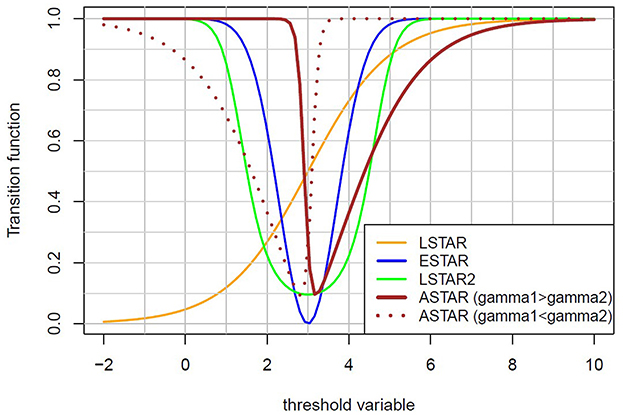
Figure 1. Typical behavior of the transition functions.

3 Results and discussion

3.1 Model estimation in R

tsDyn is a popular R package for non-linear time series models with regime switching. It offers estimation functions only for SETAR and LSTAR, without the option to estimate ESTAR or LSTAR2. Since R is open-source software, the code of the function lstar() for LSTAR estimation [11] can be used as a base for developing new functions to estimate other models. The function already allows for different equation orders, which is preferable to some other software functions that estimate STAR models with equal-order equations only.

3.1.1 Construction of lstar2(), estar(), and astar() functions

The function lstar() is modified into lstar2(), estar(), and astar() functions for LSTAR2, ESTAR, and ASTAR model estimation [7, 12–15].

The modification is performed using the available lstar() function code in the R documentation by making the necessary adjustments for each model specifically. These adjustments are as follows:

In the case of ASTAR, one smoothness parameter is replaced with two smoothness parameters, gamma1 and gamma2, throughout the whole program, including checking the initial parameter values set by the user, grid search, estimation, and output construction. The function code is modified by implementing the new formula of the transition function while using the two smoothness parameters mentioned above. The sigmoid() function used in lstar() is replaced with the direct formula of the new transition function. Moreover, modifications are made to the internal lstar() function gradEhat(). To create the Jacobian matrix, which is used for the optimization of coefficients α_i and β_i, gradEhat() is adjusted for the new model by adding a derivative by the new variable, replacing gamma with gamma1 and gamma2. The special dsigmoid() function for the derivative of a sigmoid function is not used anymore, but the derivatives of the new transition function are taken manually and placed in the code.

In the case of ESTAR, the number of parameters remains the same as in the initial lstar() function. Only the transition function is replaced with the new one. The sigmoid() and dsigmoid() functions are replaced with direct new functions and expressions of their derivatives with all parameters.

In the case of LSTAR2, one threshold coefficient from lstar() is replaced with two parameters, th1 and th2, throughout the entire code. The new transition function is implemented, and its derivatives are integrated into gradEhat(). The number of derivatives is increased by one due to the additional threshold parameter.

3.1.2 lstar2() and astar() function additions

A few additional improvements were made while creating the lstar2() and astar() functions. An option was added for the user to choose between two types of STAR model forms, which can be useful for interpreting the results. Namely, the transition function can be used only for the “high” regime regression, in the form of multiplier G(), or it can also be used as a multiplier for the “low” regime regression, in the form of 1 - G().

More possibilities are given to users in defining starting values for transition function variables. Specifically, an option has been added to set starting values for a part of the variables, allowing the user to define all three variables; define gamma (or gamma1 and gamma2 for ASTAR), allowing for the function to choose the threshold coefficient(s) by using grid search; or choose the starting values for the threshold th (or th1, th2 for LSTAR2), allowing the function to choose gamma (gamma1 and gamma2) by grid search.

To analyze estimated model results, summary, and predictions, and to perform a comparison with other models available in the R environment, a few more modifications are made by adjusting tsDyn:::predict.nlar(), tsDyn:::print.lstar(), and tsDyn:::print.summary.lstar() for the new models estimated by lstar2() and astar().

3.1.3 STAR model estimation with the new functions

LSTAR2, ESTAR, and ASTAR estimation is performed similarly to LSTAR model estimation using conditional least squares to estimate the coefficients. These function definitions in the R environment for users are as follows:

lstar2(x, m, d, steps, series, mL, mH, mTh, thDelay, thVar, th1, th2, gamma, trace, include, control, starting.control, tp),

estar(x, m, d, steps, series, mL, mH, mTh, thDelay, thVar, th, gamma, trace, include, control, starting control, tp), and

astar(x, m, d, steps, series, mL, mH, mTh, thDelay, thVar, th, gamma1, gamma2, trace, include, control, starting.control, tp),

where the arguments are similar to the lstar() function, except for the possible initial values of two thresholds, th1 and th2 (for lstar2), initial values of two smoothness parameters, gamma1 and gamma2 (for astar), and the type of model form, tp (1 or 2).

3.2 Data analysis

As in most other countries, the unemployment rate in Latvia, like many other economic variables, is highly unstable. It can be expected to vary across different periods, influenced by various economic and political shocks.

3.2.1 The data

Our analysis is based on publicly available monthly data of the unemployment rate among 15–75-year-old residents of Latvia for the period January 2002 to June 2025, published by the Central Statistical Bureau of Latvia [16].

Examining the shape of our data in Figure 2, we notice that it is strongly non-stationary, with breaks, likely several. Especially during the Great Financial Crisis of 2008, the unemployment rate increased sharply. Then, it gradually decreased until the COVID-19 pandemic, when it sharply increased again, although not for as long as in 2008. After a short period of gradual decrease until the spring of 2023, we observe a rather calm period, which is still continuing.

Figure 2

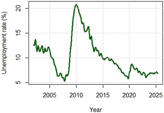
Figure 2. Unemployment rate in Latvia (2002M1–2025M5).

Such heterogeneous dynamics may require a threshold model. This is also confirmed by statistical tests. The Augmented Dickey-Fuller test cannot reject a unit root with a confidence probability larger than 0.9056. The Zivot-Andrews test, however, rejects the unit root hypothesis and supports the alternative hypothesis of a stationary series with a structural break at an unknown point in the intercept, the linear trend, or both, with a confidence probability greater than 0.95.

To remove the strong trend in the series, we take first differences (see them in Figure 3) and further analyze the changes in the unemployment rate, constructing models based on them.

Figure 3

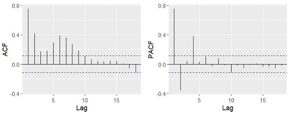
Figure 3. Autocorrelation (ACF) and partial autocorrelation function (PACF) of the differences in unemployment rate.

Currently, the Augmented Dickey–Fuller test rejects the unit root with a p-value of 0.026.

Although we do not see strong evidence of non-stationarity in the correlogram (autocorrelation and partial autocorrelation functions; Figure 4), at least in the first 18 lags, Tsay's test rejects the null hypothesis that the time series follows an autoregressive process and accepts the alternative hypothesis of non-linearity with a p-value close to zero (5.423247e-07).

Figure 4

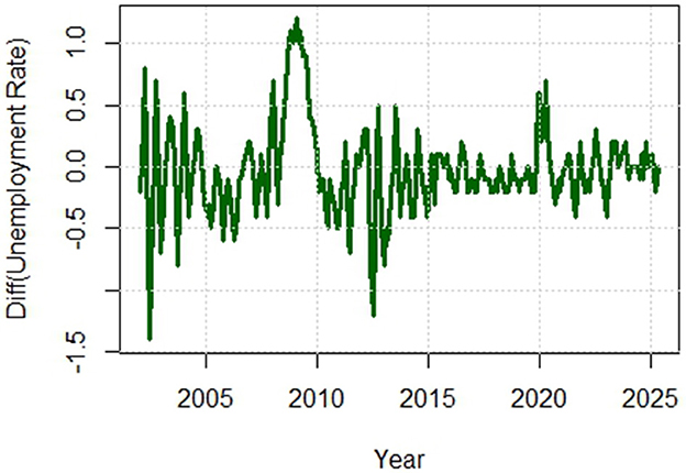
Figure 4. Differences in the unemployment rate in Latvia (2002M2–2025M5).

The Zivot–Andrews test rejects a unit root in the series of differences and accepts the alternative hypothesis of a stationary series with a break at an unknown point with a confidence probability larger than 0.99.

Then, the threshold non-linearity test rejects H₀ of being an autoregressive process and accepts H₁ of being a threshold autoregressive model for all lags up to at least 12, with p-values close to zero. Moreover, the special Terasvirta [6] non-linearity test is applied to test non-linearity against STAR models and to choose among the smooth transition models. By testing regression orders up to 12, linearity is rejected for all of them.

As follows from the tests, a threshold or smooth transition autoregressive model can describe our data better than linear autoregressive models.

3.2.2 Model choice and comparison

Henceforth, the period up to August 2024 is used as the training period to estimate the models, and the last 9 months are used as the testing period.

The Terasvirta [6] test shows mixed results when choosing between the LSTAR and ESTAR models. Specifically, the primary test based on Terasvirta's Taylor expansion selection procedure suggests the LSTAR, but an auxiliary test points to ESTAR as the model most likely to have the best fit. The best decision in this case is to estimate and compare both models. Additionally, ARIMA, SARIMA, ARMA+GARCH, SETAR, LSTAR2, and ASTAR of the best possible order and parameters, with possibly better properties (full, stationary, parsimonious), are estimated for comparison. Models of all types with orders less than 4 are not full, but orders greater than 4 appear less parsimonious. Additionally, the constant term, which allows for a non-zero intercept, is kept in all models, despite being insignificant for some of them, because its inclusion may improve predictive performance [9, 10]. The model selection procedure for each type of model includes the estimation of various models and different validity tests to exclude the presence of unit roots, residual correlation, squared residual correlation, and heteroscedasticity. Candidate models are compared with information criteria, RMSE, residual variance, and significance of coefficients. A manual comparison is preferred over an automatic procedure for more thorough information processing and to maintain a similar structure when choosing among valid and equally or almost equally good models. The first lag of unemployment rate changes is used as a threshold variable that has an economic justification. Finally, the following models are chosen:

AR(4)

$\begin{array}{l}{Y}_t=-0.0221+1.0499Y_{t-1}-0.2497Y_{t-2}-0.4103Y_{t-3}\\ +0.4216Y_{t-4}+w_t,\end{array}$

SARIMA(1,0,3)(2,0,0)[12]

$\begin{array}{r}\left(1+0.0009B^{12}-0.0647B^{24}\right)\left(1-0.8974B\right)Y_t\\ =\left(1+0.1502B-0.1963B^2-0.4152B^3\right)w_t\end{array}$

The best chosen SARIMA model is excluded from further consideration and comparison because it is not full, its seasonal terms are not significant, and any changes in orders do not make the seasonal terms significant.

AR(4)+GARCH(1,1)

$\begin{array}{l}{Y}_t=-0.008+1.0137Y_{t-1}-0.1865Y_{t-2}-0.3538Y_{t-3}\\ +0.3133Y_{t-4}+w_t\\ w_t={\nu }_t\sqrt{h_t,}\\ h_t=0.0058+0.2478w_{t-1}^2+0.6033h_{t-1}\end{array}$

SETAR

$\begin{array}{l}{Y}_t=\{\begin{array}{c}-0.0711+0.7757Y_{t-1}-0.201Y_{t-2}-0.4337Y_{t-3}\\ +0.2534Y_{t-4}+w_t^{(1)},& if{Y}_{t-1}\le 0\\ -0.0288+1.2005Y_{t-1}-0.2838Y_{t-2}-0.3865Y_{t-3}\\ +0.4219Y_{t-4}+w_t^{(2)},& if{Y}_{t-1}>0\end{array}\end{array}$

LSTAR

$\begin{array}{l}{Y}_t=-0.1026+0.7299Y_{t-1}-0.2258Y_{t-2}-0.4204Y_{t-3}\\ +0.3608Y_{t-4}\\ +\frac{1}{1+e^{-24.0836(Y_{t-1}+0.111)}}\\ \left[0.0718+0.486Y_{t-1}-0.0163Y_{t-2}\right]+w_t,\end{array}$

LSTAR2

$\begin{array}{l}{Y}_t=-0.0287+1.0161Y_{t-1}-0.2609Y_{t-2}-0.3914Y_{t-3}\\ +0.2848Y_{t-4}\\ +\left(\frac{1}{1+e^{-10.0012(Y_{t-1}+0.8979)(Y_{t-1}-0.835)}}\right)\\ \left[0.3543-0.4202Y_{t-1}+0.4808\right]+w_t,\end{array}$

ESTAR

$\begin{array}{l}{Y}_t=-0.0431+1.2628Y_{t-1}-0.3976Y_{t-2}-0.4942Y_{t-3}\\ +0.3453Y_{t-4}\\ +\left(\frac{1}{1+e^{-{4(Y_{t-1}-0.1)}^2}}\right)\\ \left[0.1211-0.4221Y_{t-1}+0.4343Y_{t-2}\right]+w_t,\end{array}$

ASTAR

$\begin{array}{l}{Y}_t=-0.0108+1.1365Y_{t-1}-0.2411Y_{t-2}-0.3789Y_{t-3}\\ +0.3517Y_{t-4}\\ +\left(1-\frac{1.5}{1+0.5e^{-15.0001(Y_{t-1}+0.5098)}+0.5e^{0.0144(Y_{t-1}+0.5098)}}\right)\\ \left[-0.3495-0.4744Y_{t-1}-0.5494Y_{t-2}\right]+w_t.\end{array}$

Comparing the fit of the chosen AR(4), AR(4)+GARCH(1,1), LSTAR, SETAR, LSTAR2, ESTAR, and ASTAR models using the root mean squared error loss (RMSE), (unconditional) residual variance (RV), and Akaike Information Criterion (AIC), LSTAR2 displays the best goodness-of-fit (Table 1). ASTAR is the second best according to RMSE.

Table 1

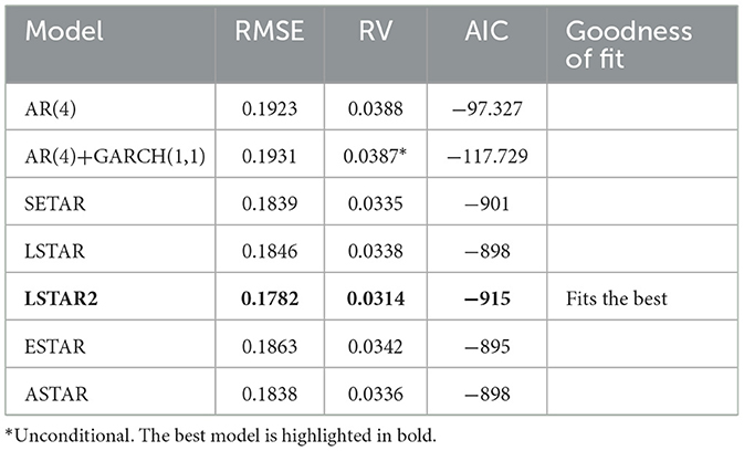
Table 1. Comparison of models with RMSE, RV, and AIC (using lag1 as a threshold variable for STAR and SETAR).

Taking into account the economic relationship between unemployment and inflation and the possibility of using an external variable as the threshold function, the STAR models are fitted using inflation as a threshold variable. The necessary inflation data for the period from February 2002 to June 2025 are retrieved from the site of the Central Statistical Bureau of Latvia [17]. However, there is no improvement when comparing the STAR models with the previously chosen LSTAR2 model (see Table 2).

Table 2

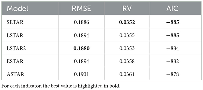
Table 2. Comparison of models with RMSE (using inflation as a threshold variable for STAR and SETAR).

Therefore, there is no reason to use inflation as a threshold variable in the considered STAR models.

3.2.3 Analysis of the best model

The majority of the coefficients of the estimated best-chosen LSTAR2 model are statistically significant (Table 3).

Table 3

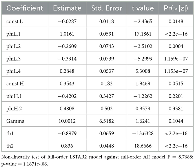
Table 3. Estimates of the coefficients of the chosen LSTAR2 model.

The non-linearity test rejects the linear autoregressive model and accepts the logistic smooth transition model, with a p-value of 1.1871e-06. The thresholds are estimated as −0.8979 and 0.836. Therefore, −0.031 is the level primarily corresponding to the second regime. The smoothness coefficient is 10.0012, indicating a moderate transition, which means that the transition is neither too fast nor too slow.

The number of estimated coefficients in the regimes of the chosen LSTAR2 model is different, which leads to a more parsimonious model. Some coefficients remain insignificant because, by excluding them from the model, the estimation procedure does not converge.

According to the Diebold–Mariano test for predictive accuracy of the constructed models for in-sample one-step forecasts in the sample period until August 2024, one can reject the null hypothesis that the two models have the same forecast accuracy and accept the alternative that the LSTAR2 forecast is more accurate than the LSTAR forecast with a p-value of 0.04368 and is more accurate than ASTAR with a p-value of 0.04562.

In Figure 5, the data with forecasts for nine steps, i.e., for the period September 2024–May 2025, are based on the previous data. The ESTAR, AR, and GARCH forecasts tend to be rather high, whereas the LSTAR forecast is the lowest. For the first three moments, nearly all models except ESTAR recognize the decrease in the change in unemployment rate rather well. Furthermore, they become more spread and fail to capture fluctuations accurately, yet they do not deviate far from the real values.

Figure 5

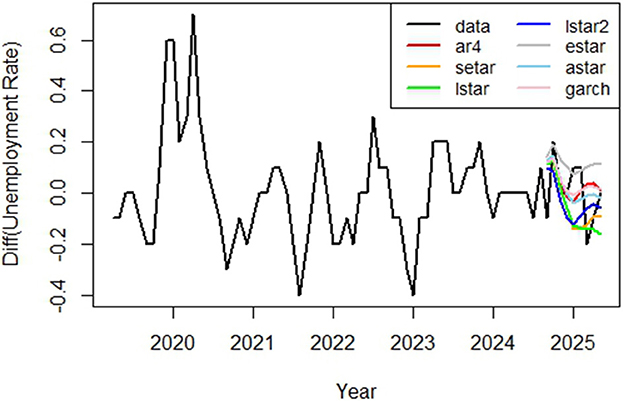
Figure 5. Forecast of the difference in unemployment by different models.

The RMSEs of the forecasts for different horizons ranging from 3 to 9 by the chosen STAR and SETAR models are presented in Table 4. We see that LSTAR2 gives the best RMSE for short horizons (3 and 4). Furthermore, ASTAR mostly appears to be the best. Moreover, it has the lowest average RMSE among all STAR and SETAR models. Thus, the ASTAR forecast is better for the longer period.

Table 4

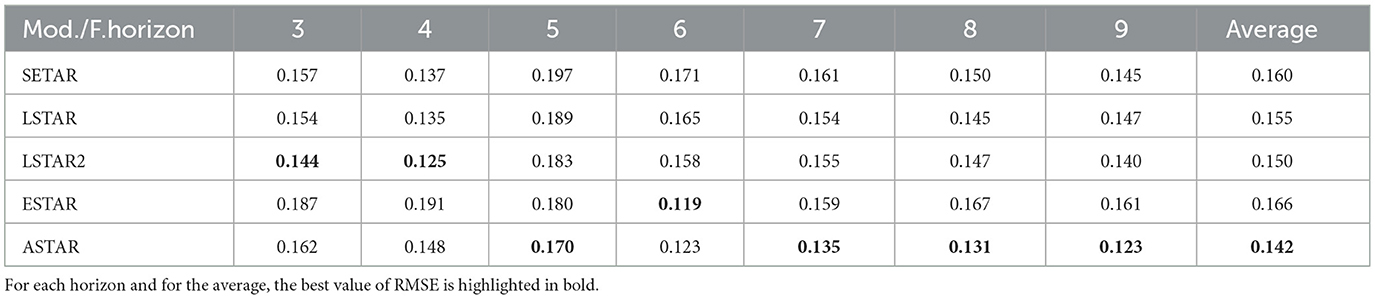
Table 4. Forecast RMSE of the difference in unemployment by different models.

Figure 6 shows the prediction of the difference in the unemployment rate for the next 9 months based on all available data up to May 2025. We see that the forecasts have similar patterns, predicting the highest value in June, followed by a decrease until October, with a small, slower but gradual increase until January, with a possible turn again, with the ESTAR, AR, and GARCH forecasts remaining more pessimistic (with a larger increase in the unemployment rate). According to the other models, the difference is predicted to be negative, which means a decrease in the unemployment rate. Considering that the unemployment rate was less than 7% over the last few months, our forecasts may indicate economic overheating.

Figure 6

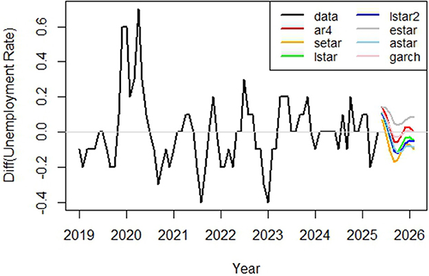
Figure 6. Forecast of the future values of the difference in unemployment by different models.

4 Conclusion

The differences in the unemployment rate in Latvia are explored with various tests, proving that they have structural breaks and follow a threshold or a smooth transition model.

The second-order logistic smooth transition autoregressive model is found to have a better fit for these series than linear autoregression with and without conditionally heteroscedastic errors, better than the self-exciting threshold autoregression, the smooth transition autoregressive model with a logistic transition function of the first order, the exponential smooth transition autoregression, and the asymmetric smooth transition autoregression. However, the best out-of-sample forecast, according to the average RMSE, considering horizons from 3 to 9, is given by the ASTAR model.

The conducted analysis illustrates that the new asymmetric transition function ASTAR for the STAR model, as well as the recently developed R estimation procedures for LSTAR2, ESTAR, and ASTAR, are useful for modeling and forecasting financial data with structural shifts. The built-in option to use different orders for the regimes' equations allows choosing more parsimonious models.

5 Future research directions

Future research could investigate the use of the STAR models, particularly with the new ASTAR transition function, across a broader range of economic and financial data to better assess their utility for different datasets. Enhancing estimation methods, especially in how parameter restrictions are managed, could improve the accuracy and reliability of estimated models. Additionally, the asymmetric transition function requires further examination to better understand its behavior and to make any necessary adjustments.

Data availability statement

Publicly available datasets were analyzed in this study. This data can be found at: https://data.stat.gov.lv/pxweb/lv/OSP_PUB/START__EMP__NBBA__NBBB/NBB150m/.

Author contributions

OP: Conceptualization, Formal analysis, Investigation, Methodology, Software, Validation, Visualization, Writing – original draft.

Funding

The author(s) declare that no financial support was received for the research and/or publication of this article.

Conflict of interest

The author declares that the research was conducted in the absence of any commercial or financial relationships that could be construed as a potential conflict of interest.

Generative AI statement

The author(s) declare that no Gen AI was used in the creation of this manuscript.

Any alternative text (alt text) provided alongside figures in this article has been generated by Frontiers with the support of artificial intelligence and reasonable efforts have been made to ensure accuracy, including review by the authors wherever possible. If you identify any issues, please contact us.

Publisher's note

All claims expressed in this article are solely those of the authors and do not necessarily represent those of their affiliated organizations, or those of the publisher, the editors and the reviewers. Any product that may be evaluated in this article, or claim that may be made by its manufacturer, is not guaranteed or endorsed by the publisher.

References

1. Enders W. Applied Econometric Time Series, 4th Edn. Hoboken, NJ: Wiley.

Google Scholar

2. Kavkler A, Mikek P, Böhm B, Boršič D. Nonlinear Econometric Models: the Smooth Transition Regression Approach. (2008). Available online at: https://www.researchgate.net/publication/228556576 (Accessed May 5, 2024).

Google Scholar

3. Aydin D, Mermi S. Some regime-switching models for economic time series: a comparative study. Eskisehir Tech Univ J Sci Technol A-Appl Sci Eng. (2022) 23:48–69. doi: 10.18038/estubtda.881251

Crossref Full Text | Google Scholar

4. Hansen G. Forecasting prices of dairy commodities – a comparison of linear and nonlinear models. Irish J Agric Food Res. (2020) 59:98–112. doi: 10.15212/ijafr-2020-0101

Crossref Full Text | Google Scholar

5. Pavlenko O, Matvejevs A. Comparison of linear and nonlinear models for forecasting of food commodity prices in Latvia. In: 22nd International Scientific Conference “Engineering for Rural Development”: Proceedings, Vol. 22, Latvia, Jelgava, May 24-26, 2023. Jelgava: Latvia University of Life Sciences and Technologies (2023). p. 735–44.

Google Scholar

6. Terasvirta T. Specification, estimation, and evaluation of smooth transition autoregressive models. J Am Stat Assoc. (1994) 89:208–18. doi: 10.2307/2291217

Crossref Full Text | Google Scholar

7. Pavlenko O. Star time series models with asymmetric transition function: estimation using R software and applications for Latvian economic data. In: 24th International Scientific Conference “Engineering for Rural Development”: Proceedings, Vol. 24, Latvia, Jelgava, May 21-23, 2025. Jelgava: Latvia University of Life Sciences and Technologies (2025). p. 457–62. doi: 10.22616/ERDev.2025.24.TF096

Crossref Full Text | Google Scholar

8. Shumway RH, Stoffer DS. Time Series Analysis and Its Applications: With R Examples, 4th Edn. Cham: Springer Science + Business Media, LLC (2017). doi: 10.1007/978-3-319-52452-8

Crossref Full Text | Google Scholar

9. Tong H. Threshold Models in Non-linear Time Series Analysis. New York, NY: Springer (1983). doi: 10.1007/978-1-4684-7888-4

Crossref Full Text | Google Scholar

10. Teräsvirta T, Anderson HM. Characterizing nonlinearities in business cycles using smooth transition autoregressive models. J Appl Econom. (1992) 7:S119–36. doi: 10.1002/jae.3950070509

Crossref Full Text | Google Scholar

11. Di Narzo AF, Aznarte JL, Stigler M. tsDyn: Nonlinear Time Series Models with Regime Switching (Version 11.0.4.1) [R package]. (2023). Available online at: https://CRAN.R-project.org/package=tsDyn (Accessed May 5, 2023).

Google Scholar

12. Zeltina L. Logistiskās Gludās Pārejas Autoregresivā Modela LSTAR2 Novērtēšanas Implementācija Rstudio un Pielietojumi Finansēs [Master's thesis]. Riga: RTU (2024).

Google Scholar

13. Pavlenko O, Zeltina L. The second order logistic smooth transition autoregressive model for unemployment rate of Latvia. In: Proceedings of the 2024 IEEE 65th International Scientific Conference on Information Technology and Management Science of Riga Technical University (ITMS 2024), 3-4 October, 2024. Latvia, Riga (2024). p. 41–5. doi: 10.1109/ITMS64072.2024.10741945

Crossref Full Text | Google Scholar

14. Pavlenko O. (2025). Available online at: https://github.com/Oksana-Pavlenko/PublicFiles/blob/main/ASTAR.R (Accessed October 3, 2025).

Google Scholar

15. Pavlenko O. (2025). Available online at: https://github.com/Oksana-Pavlenko/PublicFiles/blob/main/estar_functions.R (Accessed October 11, 2025).

Google Scholar

16. Central Statistical Bureau (CSB), Republic Republic of Latvia. The Data of Unemployed and Unemployment Rate Aged 15-74 by Sex 2002M01-2025M05. (2025). Available online at: https://data.stat.gov.lv/pxweb/lv/OSP_PUB/START__EMP__NBBA__NBBB/NBB150m/ (Accessed July 4, 2025).

Google Scholar

17. Central Statistical Bureau (CSB), Republic Republic of Latvia. Consumer Price Indices and Changes by Commodity Groups (ECOICOP) 2002M01 - 2025M05. Available online at: https://data.stat.gov.lv/pxweb/lv/OSP_PUB/START__VEK__PC__PCI/PCI020m/ (Accessed July 4, 2025).

Google Scholar