Dynamical behavior of a stochastic SEIQRV infectious model with an Ornstein-Uhlenbeck process and general incidence

Considering the influence of quarantine and vaccination factors, this study examines an SEIQRV infectious disease model that incorporates an Ornstein-Uhlenbeck process and a general incidence function. By accounting for disease-induced mortality rates among infected individuals, the article establishes the existence and uniqueness of a global solution for any arbitrary positive initial value. An adequate condition for disease extinction is also provided. Simultaneously, by reconstructing a sequence of random Lyapunov functions, we demonstrate the existence of a unique stationary distribution indicating that the disease persists over a period of time in a biological sense. Based on these findings, the precise expression for the probability density function of the stochastic model near the quasi-equilibrium state is derived. Finally, the theoretical results are verified through a series of numerical simulations.

1 Introduction

SARS-CoV-2, a coronavirus that emerged in late 2019, causes a severe respiratory illness that can progress to fatal pneumonia [1]. The WHO has characterized the epidemic as COVID-19 [2]. SARS-CoV-2, is primarily transmitted through three routes: respiratory aerosol inhalation, immediate human exposure, and droplet transmission [3]. It is worth noting that the implementation of quarantine and vaccination measures significantly influences epidemic dynamics. To understand the transmission dynamics of infectious diseases, many scholars have proposed numerous mathematical models to predict and control the development of diseases. For instance, Tang et al. [4] developed a generalized SEIR model of the SEIR-type considering isolation and treatment, which elucidated the transmission dynamics of COVID-19 and evaluated the effect of public health interventions on disease infections. Poonia et al. [5] developed a SEIRV model incorporating vaccination rate, highlighting the critical role of social distancing and vaccination in epidemic control.

In 2020, Fosu et al. [6] proposed a SEIQRV general epidemiological model for COVID-19 as follows:

$\begin{array}{ll}\{\begin{array}{l}\text{d}S=[\Lambda -\bar{\beta }SI-(\mu +\delta )S+\nu E]\text{d}t,\\ \text{d}E=[\bar{\beta }SI-({\sigma }_2+\gamma +\nu +\mu )E]\text{d}t,\\ \text{d}I=[\gamma E-({\sigma }_1+{\omega }_1+\mu )I]\text{d}t,\\ \text{d}Q=[{\sigma }_{1}I+{\sigma }_{2}E-({\omega }_2+\mu )Q]\text{d}t,\\ \text{d}R=[{\omega }_{1}I+{\omega }_{2}Q-\mu R]\text{d}t,\\ \text{d}V=[\delta S-\mu V]\text{d}t.\end{array}& (1)\end{array}$

where S(t), E(t), I(t), Q(t), R(t), and V(t) represent the number of susceptible, exposed, infected, quarantined, recovered, and vaccinated classes at time t, respectively, and their initial values are satisfied:

$\begin{array}{l}S(0)>0,E(0)>0,I(0)>0,Q(0)\ge 0,R(0)\ge 0,V(0)\ge 0.\end{array}$

The parameters of Equation 1 are defined as follows: $\bar{\beta }$ denotes the transmission rate from susceptible to exposed individuals; Λ represents the recruitment rate of susceptible populations; μ is the natural death rate; δ denotes the vaccination rate among susceptibles; ν is the transfer rate from exposed back to susceptible; γ is the progression rate from exposed to infected; σ₁ and σ₂ represent the quarantine rates for infected and exposed individuals, respectively; ω₁ and ω₂ are the recovery rates of infected and quarantined individuals, respectively.

On this basis, considering that the mechanism of disease transmission may be influenced by several factors, we introduce the disease-caused mortality rate h of infected individuals and assume that this rate exceeds the natural mortality rate. The resulting deterministic Equation 2 takes the following form:

$\begin{array}{ll}\{\begin{array}{l}\text{d}S=[\Lambda -\bar{\beta }SI-(\mu +\delta )S+\nu E]\text{d}t,\\ \text{d}E=[\bar{\beta }SI-({\sigma }_2+\gamma +\nu +\mu )E]\text{d}t,\\ \text{d}I=[\gamma E-({\sigma }_1+{\omega }_1+\mu +h)I]\text{d}t,\\ \text{d}Q=[{\sigma }_{1}I+{\sigma }_{2}E-({\omega }_2+\mu )Q]\text{d}t,\\ \text{d}R=[{\omega }_{1}I+{\omega }_{2}Q-\mu R]\text{d}t,\\ \text{d}V=[\delta S-\mu V]\text{d}t.\end{array}& (2)\end{array}$

Similar to Fosu et al. [6], here are certain conclusions about Equation 2:

(1) The basic reproduction number of Equation 2 is $R_0=\frac{\Lambda \bar{\beta }\gamma }{(\mu +\delta )({\omega }_1+{\sigma }_1+\mu +h)(\gamma +{\sigma }_2+\nu +\mu )}$.

(2) The disease-free equilibrium point is $E_0=(S_0,E_0,I_0,Q_0,R_0,V_0)=(\frac{\Lambda }{\mu +\delta },0,0,0,0,\frac{\delta \Lambda }{\mu (\mu +\delta )})$, and the disease-free equilibrium point E₀ is locally asymptotically stable for R₀ < 1.

(3) The endemic equilibrium point is P^* = (S^*, E^*, I^*, Q^*, R^*, V^*), and the endemic equilibrium point P^* is globally asymptotically stable for R₀ > 1, where $S^{*}=\frac{({\omega }_1+{\sigma }_1+\mu +h)(\gamma +{\sigma }_2+\nu +\mu )}{\bar{\beta }\gamma },E^{*}=\frac{\Lambda -(\mu +\delta )S^{*}}{\gamma +{\sigma }_2+\mu },I^{*}=\frac{\gamma E^{*}}{{\omega }_1+{\sigma }_1+\mu +h},Q^{*}=\frac{{\sigma }_1{I}^{*}+{\sigma }_2{E}^{*}}{{\omega }_2+\mu },R^{*}=\frac{{\omega }_1{I}^{*}+{\omega }_2{Q}^{*}}{\mu },V^{*}=\frac{\delta ({\omega }_1+{\sigma }_1+\mu +h)(\gamma +{\sigma }_2+\nu +\mu )}{\bar{\beta }\gamma \mu }$.

However, due to the inherent variability in real-world populations, viral transmission is subject to stochastic disturbances. Consequently, a growing body of research in infection dynamics focuses on the stochastic properties of dynamical systems. Stochastic epidemic models that incorporate environmental noise provide a more realistic representation of disease spread than traditional deterministic models [7]. For instance, Shi et al. [8] proposed a randomized COVID-19 SEIR model with an Ornstein-Uhlenbeck process, which contributes to our comprehension of the dynamic mechanisms. Su et al. [9] applied a randomized HBV infectious model having normal morbidity, cell-to-cell spread, and immunological reactions. The consequences of environmental perturbations on the mathematical model can be realized by revising the model's parameters. Two principal ways of changing the parameters are mentioned [10]. One approach is to pretend that the parameters are linear functions of Gaussian white noise. Liu et al. [11] developed an SEIR-based COVID-19 stochastic epidemic model incorporating independent standard Brownian motion to analyze transmission dynamics within infected populations. Shi et al. [12] developed a stochastic SEIRS rabies model incorporating population diffusion. The other option is to utilize the mean-reversion process to interfere with the parameters. Wei et al. [13] established the dynamic behavior of an HIV infection model featuring two transmission modes. Liu et al. [14] investigated a viral infectious disease model incorporating latent individuals and a log-OU process. Ornstein-Uhlenbeck process is notionally and biologically more relevant. It better characterizes environmental heterogeneity in biological systems than a linear function of white noise [15]. Thus, this study adopts the latter assumption. Since $\bar{\beta }$ is biologically important as the rate of transmission between susceptible and exposed individuals, then we suppose that $\bar{\beta }$ of Equation 2 varies arbitrarily due to environmental perturbations and it is amenable to the Ornstein–Uhlenbeck process. In this case, $\bar{\beta }$ could be changed to the form below:

$\begin{array}{ll}\begin{array}{l}\text{d}\beta (s)=\alpha (\bar{\beta }-\beta (s))\text{d}s+\theta \text{d}B(s),\end{array}& (3)\end{array}$

where α > 0 is for the speed of reversal. θ > 0 stands for the intensity of fluctuation. B(s) is the standard Brownian motion. The solution of Equation 3 can be expressed as follows: $\beta (s)=e^{-\alpha s}\beta (0)+(1-e^{-\alpha s})\bar{\beta }+{\int }_0^s{e}^{-\alpha (s-x)}\theta \mathrm{\text{d}}B(x)$, and $\beta (s)~N(\bar{\beta },\frac{{\theta }^2}{2\alpha })$ as s → ∞. By calculation, it is clear that when s → ∞, we have

$𝔼(\beta (s))=e^{-\alpha s}𝔼(\beta (0))+(1-e^{-\alpha s})\bar{\beta }\to \bar{\beta },Var(\beta (s))=e^{-2\alpha t}Var(\beta (0))+(1-e^{-\alpha s})\frac{{\theta }^2}{2\alpha }\to \frac{{\theta }^2}{2\alpha }$.

Based on Allen [15], β(s) is ergodic. Its asymptotic probability density function is $\pi (\chi )=\frac{\sqrt{\alpha }}{\theta \sqrt{\pi }}{e}^{-\frac{\alpha {(\chi -\bar{\beta })}^2}{{\theta }^2}}$. Assuming $\beta (0)=\bar{\beta }$. Defining $\bar{\beta }(s)$ to be the time-averaged, we have

$\begin{array}{r}\bar{\beta }(s)=\frac{1}{s}{\displaystyle {\int }_0^s}\beta (x)dx+\frac{1}{s}{\displaystyle {\int }_0^s}\frac{\theta }{\alpha }(1-e^{\alpha (x-s)})\text{d}B(x),𝔼(\bar{\beta }(s))7g5g\\ =\bar{\beta },Var(\bar{\beta }(s))=\frac{{\theta }^{2}s}{3}+o(s^2).\end{array}$

As s → 0, the variance $\mathrm{\text{Var}}(\bar{\beta }(s))$ tends to zero rather than infinity. This behavior indicates that the Ornstein-Uhlenbeck process is more suitable for characterizing the effects of stochastic perturbations. Because $\bar{\beta }$ is a normal number based on its biological significance, we know that β(s) has a significant probability of being positive by the property of the normal distribution when θ becomes small. Letting β⁺(t) = max{β(s), 0}. Adding Ornstein–Uhlenbeck process to Equation 2, we have the stochastic model as below:

$\begin{array}{ll}\{\begin{array}{l}\text{d}S=[\Lambda -{\beta }^{+}(t)SI-(\mu +\delta )S+\nu E]\text{d}t,\\ \text{d}E=[{\beta }^{+}(t)SI-({\sigma }_2+\gamma +\nu +\mu )E]\text{d}t,\\ \text{d}I=[\gamma E-({\sigma }_1+{\omega }_1+\mu +h)I]\text{d}t,\\ \text{d}Q=[{\sigma }_{1}I+{\sigma }_{2}E-({\omega }_2+\mu )Q]\text{d}t,\\ \text{d}R=[{\omega }_{1}I+{\omega }_{2}Q-\mu R]\text{d}t,\\ \text{d}V=[\delta S-\mu V]\text{d}t,\\ \text{d}\beta (t)=\alpha (\bar{\beta }-\beta (t))dt+\theta \text{d}B(t).\end{array}& (4)\end{array}$

Since the sixth expression in Equation 4 does not affect the dynamical analysis, we only have to investigate the stochastic model as follows:

$\begin{array}{ll}\{\begin{array}{l}\text{d}S=[\Lambda -{\beta }^{+}(t)SI-(\mu +\delta )S+\nu E]\text{d}t,\\ \text{d}E=[{\beta }^{+}(t)SI-({\sigma }_2+\gamma +\nu +\mu )E]\text{d}t,\\ \text{d}I=[\gamma E-({\sigma }_1+{\omega }_1+\mu +h)I]\text{d}t,\\ \text{d}Q=[{\sigma }_{1}I+{\sigma }_{2}E-({\omega }_2+\mu )Q]\text{d}t,\\ \text{d}R=[{\omega }_{1}I+{\omega }_{2}Q-\mu R]\text{d}t,\\ \text{d}\beta (t)=\alpha (\bar{\beta }-\beta (t))dt+\theta \text{d}B(t).\end{array}& (5)\end{array}$

The remaining parts of the article are structured according to the following description. Section 2 investigates whether a unique global solution exists for Equation 5. Section 3 gives an adequate condition for the extinction of the epidemic. Section 4 derives a stationary distribution for the Equation 5, which describes the continuation of the disorder. Section 5 derives the exact expression of the probability density function through solving the relevant six-dimensional Fokker–Planck equation. Section 6 illustrates theoretical outcomes with a few numerical simulations. Section 7 ends with several conclusions.

2 Existence of unique global solution

To analyze the dynamic behavior of Equation 5, it is necessary first to establish the existence of a global solution. This is a fundamental requirement for all subsequent proofs. Let $\mathcal{M}(t)=(S(t),E(t),I(t),Q(t),R(t),\beta (t))$.

Theorem 2.1. For any initial value $\mathcal{M}(0)\in {ℝ}_{+}^5\times ℝ$ , there will exist a unique global solution $\mathcal{M}(t)$ for Equation 5, and it will stay in ${ℝ}_{+}^5\times ℝ$ with probability one.

Proof. Since the coefficients of system (1.5) are locally Lipschitz continuous on ℝ⁵+ × ℝ for any initial value $\mathcal{M}(0)\in {ℝ}^5+\times ℝ$, it follows that there exists a unique local solution $\mathcal{M}(t)$ on t ∈ [0, τ_e), where τ_e denotes the explosion time. To justify that $\mathcal{M}(t)$ is global, we simply prove τ_e = ∞ a.s..

Let k₁ > 0 be large enough to ensure $\mathcal{M}(0)\in {ℝ}_{+}^5\times ℝ$ remains inside the interval $[\frac{1}{k_1},k_1]$. Then, for every integer m ≥ k₁, define a stopping time as follows:

$\begin{array}{l}{\tau }_m=\inf \{t\in [0,{\tau }_e]:\min \{S(t),E(t),I(t),Q(t),R(t),e^{\beta (t)}\}\le \frac{1}{m}\\ \text{\hspace{0.17em}\hspace{0.17em}\hspace{0.17em}\hspace{0.17em}\hspace{0.17em}\hspace{0.17em}\hspace{0.17em}\hspace{0.17em}\hspace{0.17em}\hspace{0.17em}\hspace{0.17em}\hspace{0.17em}\hspace{0.17em}\hspace{0.17em}\hspace{0.17em}\hspace{0.17em}\hspace{0.17em}\hspace{0.17em}\hspace{0.17em}\hspace{0.17em}\hspace{0.17em}\hspace{0.17em}\hspace{0.17em}\hspace{0.17em}\hspace{0.17em}\hspace{0.17em}\hspace{0.17em}\hspace{0.17em}\hspace{0.17em}\hspace{0.17em}\hspace{0.17em}\hspace{0.17em}\hspace{0.17em}\hspace{0.17em}\hspace{0.17em}\hspace{0.17em}or }\max \{S(t),E(t),I(t),Q(t),R(t),e^{\beta (t)}\}\ge m\}.& (6)\end{array}$

Set infϕ = ∞(where ϕ represents the empty set). Obviously, τ_m increases monotonically with m → ∞. Define ${\tau }_{\infty }=\underset{m\to \infty }{lim}{\tau }_m$, that is, τ_∞ ≤ τ_e. In case we demonstrate that τ_∞ = ∞, then τ_e = ∞, indicating that $\mathcal{M}(t)$ is global and $\mathcal{M}(t)\in {ℝ}_{+}^5\times ℝ$.

Now, assume for contradiction that there exist constants $\bar{T}>0$, ε_m ∈ (0, 1) obeys $\mathbb{P}\left\{{\tau }_{\infty }\le \bar{T}\right\}>{\epsilon }_m$. Accordingly, there is an integer k₂ ≥ k₁ such that $\mathbb{P}\left\{{\tau }_{\infty }\le \bar{T}\right\}\ge {\epsilon }_m,\forall m\ge k_2$. What's more, ∀m ≥ k₁, t ≤ τ_m, there has

$\begin{array}{r}\frac{\text{d}(S+E+I+Q+R)}{\text{d}t}\le \Lambda -\mu (S+E+I+Q+R)-\delta S\le \Lambda \\ -\mu (S+E+I+Q+R)& (7)\end{array}$

then

$\begin{array}{ll}\begin{array}{c}S(t)+E(t)+I(t)+Q(t)+R(t)\le \frac{\Lambda }{\mu },\end{array}& (8)\end{array}$

where $S(0)+E(0)+I(0)+Q(0)+R(0)\le \frac{\Lambda }{\mu }$. Then define a non-negative C²-function $\mathcal{U}(S,E,I,Q,R,\beta ):{ℝ}_{+}^5\times ℝ\to {ℝ}_{+}$, as follows:

$\begin{array}{l}\mathcal{U}(S,E,I,Q,R,\beta )=S-1-lnS+E-1-lnE+I-1\\ -lnI+Q-1-lnQ\\ +R-1-lnR+\frac{{\beta }^2(t)}{2}\end{array}$

Set $A=\underset{\beta \in R}{sup}\{(\alpha \bar{\beta }+\frac{\Lambda }{\mu })\mid \beta (t)\mid -\alpha \mid \beta (t){\mid }^2\}$. Using Itô's formula, we obtain

$\begin{array}{ll}\begin{array}{l}L\mathcal{U}=(1-\frac{1}{S})\text{d}S+(1-\frac{1}{E})\text{d}E+(1-\frac{1}{I})\text{d}I+(1-\frac{1}{Q})\text{d}Q\\ +(1-\frac{1}{R})\text{d}R+\beta (t)\text{d}\beta (t)+\frac{1}{2}{\theta }^2\\ =\Lambda -\mu (S+E+I+Q+R)-\delta S-\frac{\Lambda }{S}+{\beta }^{+}(t)I+(\delta +\mu )\\ -\frac{\nu E}{S}-\frac{{\beta }^{+}(t)SI}{E}\\ +({\sigma }_2+\gamma +\nu +\mu )-\frac{\gamma E}{I}+({\sigma }_1+{\omega }_1+\mu +h)-\frac{{\sigma }_{1}I}{Q}\\ -\frac{{\sigma }_{2}E}{Q}+({\omega }_2+\mu )-\frac{{\omega }_{1}I}{R}\\ -\frac{{\omega }_{2}Q}{R}+\mu +\alpha \beta (t)(\bar{\beta }-\beta (t))+\frac{1}{2}{\theta }^2\\ \le \Lambda +{\beta }^{+}(t)\frac{\Lambda }{\mu }+(\delta +\mu )+({\sigma }_2+\gamma +\nu +\mu )\\ +({\sigma }_1+{\omega }_1+\mu +h)\\ +({\omega }_2+\mu )+\mu +\alpha \beta (t)(\bar{\beta }-\beta (t))+\frac{1}{2}{\theta }^2\\ \le (\alpha \bar{\beta }+\frac{\Lambda }{\mu })\mid \beta (t)\mid -\alpha \mid \beta (t){\mid }^2+\Lambda +5\mu +\delta +\gamma \\ +\nu +h+{\omega }_1+{\omega }_2+{\sigma }_1+{\sigma }_2+\frac{1}{2}{\theta }^2\\ \le A+\Lambda +5\mu +\delta +\gamma +\nu +h+{\omega }_1+{\omega }_2+{\sigma }_1+{\sigma }_2+\frac{1}{2}{\theta }^2\\ :=\tilde{k}.\end{array}& (9)\end{array}$

Here, $\tilde{k}$ is a positive constant. Integrating inequality from 0 to t and taking the expectation on both sides

$\begin{array}{l}0\le 𝔼[\mathcal{U}(S({\tau }_m\wedge \overline{T}),E({\tau }_m\wedge \overline{T}),I({\tau }_m\wedge \overline{T}),Q({\tau }_m\wedge \overline{T}),R({\tau }_m\wedge \overline{T}),\\ \beta ({\tau }_m\wedge \overline{T}))]\\ =𝔼[\mathcal{U}(ℳ(0))]+𝔼[{\displaystyle {\int }_0^{{\tau }_m\wedge \overline{T}}L}\mathcal{U}(ℳ(\tau ))d\tau ]\\ \le 𝔼[\mathcal{U}(ℳ(0))]+\tilde{k}\overline{T}.\end{array}$

For m ≥ k₂, let ${\Omega }_m={\tau }_m\le \bar{T}$, and there exists ℙ(Ω_m) ≥ ε_m. Thus for any ξ ∈ Ω_m, there exists at minimum one in $(S({\tau }_m,\xi ),E({\tau }_m,\xi ),I({\tau }_m,\xi ),Q({\tau }_m,\xi ),R({\tau }_m,\xi ),e^{\beta ({\tau }_m,\xi )})$ reaches either m or $\frac{1}{m}$. So

$\begin{array}{l}𝔼[\mathcal{U}(ℳ(0))]+\tilde{k}\overline{T}\\ \ge 𝔼[\mathcal{U}(S({\tau }_m\wedge \overline{T}),E({\tau }_m\wedge \overline{T}),I({\tau }_m\wedge \overline{T}),Q({\tau }_m\wedge \overline{T}),R({\tau }_m\wedge \overline{T}),\\ \beta ({\tau }_m\wedge \overline{T}))]\\ \ge 𝔼[1_{{\Omega }_m(\xi )}U(S({\tau }_m\wedge \overline{T}),E({\tau }_m\wedge \overline{T}),I({\tau }_m\wedge \overline{T}),Q({\tau }_m\wedge \overline{T}),\\ R({\tau }_m\wedge \overline{T}),\beta ({\tau }_m\wedge \overline{T}))]\\ \ge \epsilon [(m-1-\ln m)\wedge (\frac{1}{m}-1+\ln m)\wedge \frac{1}{4}(\ln m{)}^4].\end{array}$

When m → ∞, we can obtain $+\infty <𝔼[\mathcal{U}(\mathcal{M}(0))]+\tilde{k}\bar{T}<+\infty$. Thus, τ_∞ = +∞ a.s.; that is, τ_e = +∞. Hence, the Equation 5 admits a unique global solution $\mathcal{M}(t)$.

Remark 2.1. By Theorem 2.1, we know that Equation 5 has a unique global solution $\mathcal{M}(t)\in {ℝ}_{+}^5\times ℝ$. And if $S(0)+E(0)+I(0)+Q(0)+R(0)\le \frac{\Lambda }{\mu }$, there has $S(t)+E(t)+I(t)+Q(t)+R(t)\le \frac{\Lambda }{\mu }$. Thus, we assume that $T^{*}=\{(S,E,I,Q,R,\beta )\in {ℝ}_{+}^5\times ℝ:0<S+E+I+Q+R\le \frac{\Lambda }{\mu }\}$ is the invariant set.

3 Extinction

Having established the existence and uniqueness of the system's solution, this section presents the sufficient conditions for eradicating COVID-19, providing a theoretical basis for targeted disease control efforts. Define

$\begin{array}{l}{R}_0^E=\sqrt{R_0}+\\ \frac{\gamma \theta \Lambda }{\mu ({\sigma }_2+\gamma +\nu +\mu )\sqrt{R_0\pi \alpha }min\left\{{\sigma }_2+\gamma +\nu +\mu ,{\sigma }_1+{\omega }_1+\mu +h\right\}}.\end{array}$

Theorem 3.1. If $R_0^E<1$ , it has

$\begin{array}{r}{\displaystyle \underset{t\to \infty }{limsup}}\frac{ln(\frac{\overline{{\omega }_1}}{{\sigma }_2+\gamma +\nu +\mu }E+\frac{\overline{{\omega }_2}}{{\sigma }_1+{\omega }_1+\mu +h}I)}{t}\\ \le min\left\{{\sigma }_2+\gamma +\nu +\mu ,{\sigma }_1+{\omega }_1+\mu +h\right\}(R_0^E-1)<0,\end{array}$

, where $\overline{{\omega }_1}=\frac{\gamma }{({\sigma }_1+{\omega }_1+\mu +h)\sqrt{R_0}}$ , ${\bar{\omega }}_2=1$.

Proof. Define

$\begin{array}{l}Y(E,I)=\frac{\overline{{\omega }_1}}{{\sigma }_2+\gamma +\nu +\mu }E+\frac{{\overline{\omega }}_2}{{\sigma }_1+{\omega }_1+\mu +h}I.\end{array}$

Then $\frac{\overline{{\omega }_1}}{{\sigma }_2+\gamma +\nu +\mu }\frac{E}{Y}+\frac{{\overline{\omega }}_2}{{\sigma }_1+{\omega }_1+\mu +h}\frac{I}{Y}=1$, which means $\frac{I}{Y}<\frac{{\sigma }_1+{\omega }_1+\mu +h}{{\overline{\omega }}_2}$. Next, define the matrix M₀ as follows:

$\begin{array}{l}\left(\begin{array}{cc}0& \frac{\overline{\beta \Lambda }}{\mu ({\sigma }_2+\gamma +\nu +\mu )}\\ \frac{\gamma }{{\sigma }_1+{\omega }_1+\mu +h}& 0\end{array}\right).\end{array}$

By direct calculation, one can obtain Equation 10:

$\begin{array}{ll}\begin{array}{l}({\overline{\omega }}_1,{\overline{\omega }}_2)(M_0-{𝕀}_2)\left(\begin{array}{c}E\\ I\end{array}\right)=(\sqrt{R_0}-1)({\overline{\omega }}_{1}E+{\overline{\omega }}_{2}I).\end{array}& (10)\end{array}$

Using Itô's formula to ln Y, we have

$\begin{array}{l}L(\ln Y)=\frac{1}{Y}(\frac{{\overline{\omega }}_1{\beta }^{+}(t)SI}{({\sigma }_2+\gamma +\nu +\mu )}-{\overline{\omega }}_{1}E\\ +\frac{{\overline{\omega }}_2\gamma E}{{\sigma }_1+{\omega }_1+\mu +h}-{\overline{\omega }}_{2}I)\\ \le \frac{1}{Y}(\frac{{\overline{\omega }}_1\overline{\beta }\Lambda I}{\mu ({\sigma }_2+\gamma +\nu +\mu )}-{\overline{\omega }}_{1}E+\frac{{\overline{\omega }}_2\gamma E}{{\sigma }_1+{\omega }_1+\mu +h}\\ -{\overline{\omega }}_{2}I)+\frac{1}{Y}\frac{{\overline{\omega }}_1({\beta }^{+}(t)-\overline{\beta })\Lambda I}{\mu ({\sigma }_2+\gamma +\nu +\mu )}\\ =\frac{1}{Y}({\overline{\omega }}_1,{\overline{\omega }}_2)(M_0-{𝕀}_2)\left(\begin{array}{c}E\\ I\end{array}\right)+\frac{1}{Y}\frac{{\overline{\omega }}_1({\beta }^{+}(t)-\overline{\beta })\Lambda I}{\mu ({\sigma }_2+\gamma +\nu +\mu )}\\ \le \frac{1}{Y}(\sqrt{R_0}-1)({\overline{\omega }}_{1}E+{\overline{\omega }}_{2}I)+\frac{I}{Y}\frac{{\overline{\omega }}_1\mid \beta (t)-\overline{\beta }\mid \Lambda }{\mu ({\sigma }_2+\gamma +\nu +\mu )}\\ \le \frac{{\overline{\omega }}_{1}E+{\overline{\omega }}_{2}I}{\frac{{\overline{\omega }}_1}{{\sigma }_2+\gamma +\nu +\mu }E+\frac{{\overline{\omega }}_2}{{\sigma }_1+{\omega }_1+\mu +h}I}(\sqrt{R_0}-1)\\ +\frac{{\sigma }_1+{\omega }_1+\mu +h}{{\overline{\omega }}_2}\frac{{\overline{\omega }}_1\mid \beta (t)-\overline{\beta }\mid \Lambda }{\mu ({\sigma }_2+\gamma +\nu +\mu )}\\ \le \min \{{\sigma }_2+\gamma +\nu +\mu ,{\sigma }_1+{\omega }_1+\mu +h\}(\sqrt{R_0}-1)\\ +\frac{{\sigma }_1+{\omega }_1+\mu +h}{{\overline{\omega }}_2}\frac{{\overline{\omega }}_1\mid \beta (t)-\overline{\beta }\mid \Lambda }{\mu ({\sigma }_2+\gamma +\nu +\mu )}\\ \le \min \{{\sigma }_2+\gamma +\nu +\mu ,{\sigma }_1+{\omega }_1+\mu +h\}(\sqrt{R_0}-1)\\ +\frac{\gamma \Lambda }{(\mu ({\sigma }_2+\gamma +\nu +\mu )\sqrt{R_0}}\mid \beta (t)-\overline{\beta }\mid .& (11)\end{array}$

Integrating from 0 to t and dividing by t on both sides, we obtain

$\begin{array}{ll}\begin{array}{l}\frac{lnY(t)-lnY(0)}{t}\le min\{{\sigma }_2+\gamma +\nu +\mu ,{\sigma }_1+{\omega }_1+\mu +h\}\\ (\sqrt{R_0}-1)\\ +\frac{\gamma \Lambda }{\mu ({\sigma }_2+\gamma +\nu +\mu )\sqrt{R_0}}\frac{1}{t}{\displaystyle {\int }_0^t}\mid \beta (\tau )-\bar{\beta }\mid \text{d}\tau .\end{array}& (12)\end{array}$

Taking the superior limit,

$\begin{array}{l}\underset{t\to +\infty }{\lim \sup }\frac{\ln Y(t)}{t}\\ \le \min \{{\sigma }_2+\gamma +\nu +\mu ,{\sigma }_1+{\omega }_1+\mu +h\}(\sqrt{R_0}-1)\\ +\frac{\gamma \Lambda }{\mu ({\sigma }_2+\gamma +\nu +\mu )\sqrt{R_0}}\frac{\theta }{\sqrt{\pi \alpha }}\\ =\min \{{\sigma }_2+\gamma +\nu +\mu ,{\sigma }_1+{\omega }_1+\mu +h\}(\sqrt{R_0}\\ +\frac{\gamma \Lambda \theta }{\mu ({\sigma }_2+\gamma +\nu +\mu )\sqrt{R_0\pi \alpha }\min \{{\sigma }_2+\gamma +\nu +\mu ,{\sigma }_1+{\omega }_1+\mu +h\}}-1)\\ \min \{{\sigma }_2+\gamma +\nu +\mu ,{\sigma }_1+{\omega }_1+\mu +h\}(\sqrt{R_0^E}-1),& (13)\end{array}$

where $R_0^E=\sqrt{R_0}+\frac{\gamma \theta \Lambda }{\mu ({\sigma }_2+\gamma +\nu +\mu )\sqrt{R_0\pi \alpha }min\{{\sigma }_2+\gamma +\nu +\mu ,{\sigma }_1+{\omega }_1+\mu +h\}}$. Thus if $R_0^E<1$ , we can obtain $\underset{t\to +\infty }{lim\; sup}\frac{lnY(t)}{t}\le min\{{\sigma }_2+\gamma +\nu +\mu ,{\sigma }_1+{\omega }_1+\mu +h\}(\sqrt{R_0^E}-1)<0\mathrm{\text{a.s.}}$. That means $\underset{t\to +\infty }{lim\; sup}\frac{lnE(t)}{t}<0,\underset{t\to +\infty }{lim\; sup}\frac{lnI(t)}{t}<0\mathrm{\text{a.s.}}$, which is to say that $\underset{t\to +\infty }{lim}E(t)=0$, $\underset{t\to +\infty }{lim}I(t)=0$. This indicates that the disease ultimately becomes extinct with probability one. For COVID-19, achieving eradication requires maintaining $R_0^E<1$ over the long term. From a mathematical theory perspective, the eradication of COVID-19 is feasible. However, in the real world, achieving this goal is extremely challenging due to complex environmental factors, including population mobility, viral mutations, and animal reservoirs. It is crucial to note that $R_0^E<1$ describes the epidemic's transmission trend, not the instantaneous infection status. In the short term, residual infected individuals may persist within the population. However, due to the significantly reduced transmission efficiency of the virus, this will not trigger new large-scale outbreaks. Over time, the number of infected individuals will gradually decrease until the final infected person recovers or is eliminated, at which point the epidemic will be officially declared over.

Remark 3.1. There is $R_0^E\to \sqrt{R_0}$ as θ → 0, and $R_0^E<1$ can derive R₀ < 1. This indicates that $R_0^E<1$ can be regarded as a unifying criterion for both deterministic and stochastic models of disease extinction.

4 Stationary distribution

Deterministic models have been effective in capturing the continuity of COVID-19 infection dynamics. However, such models do not possess a fixed equilibrium state in the stochastic sense, due to the inherent randomness in disease transmission and progression. To more accurately characterize the long-term behavior of the epidemic under uncertainty, we turn to the concept of a stationary distribution within the stochastic framework. In this section, we derive sufficient conditions for the existence and stability of a stationary distribution for the stochastic system described by Equation 5. These conditions provide theoretical insights into the circumstances under which the infection is likely to persist endemically over time.

Lemma 4.1. ([16–18]) For any initial value $X(0)=X_0\in T^{*}$, assuming there is a bounded closed domain Γ∈T^* with a regular boundary, if

$\begin{array}{l}{\displaystyle \underset{t\to \infty }{lim inf}}\frac{1}{t}{\displaystyle {\int }_0^t}\mathbb{P}(x,X_0,\Gamma )\text{d}x>0,\text{a.s.},\end{array}$

where ℙ(x, X₀, Γ) is the transition probability of X(t). That means Equation 5 has at least one ergodic stationary distribution.

Define

$\begin{array}{ll}{R}_0^S=\frac{\tilde{\beta }\Lambda \gamma }{(\delta +\mu )({\sigma }_1+{\omega }_1+\mu +h)({\sigma }_2+\gamma +\nu +\mu +c_1\frac{\Lambda \theta }{\mu \sqrt{\pi \alpha }})},& (14)\end{array}$

, where $\tilde{\beta }={({\int }_0^{+\infty }{x}^{\frac{1}{4}}\pi (x)dx)}^4,c_1=\frac{\tilde{\beta }\Lambda \gamma }{{(\delta +\mu )}^2({\sigma }_1+{\omega }_1+\mu +h)}$.

Theorem 4.1. Assume $R_0^S>1$, the solution $\mathcal{M}(t)$ of Equation 5 has at least one stationary distribution π(·) on T^*.

Proof. Using Itô's formula to Equation 5,

$\begin{array}{l}\begin{array}{l}L(-lnS)=-\frac{\Lambda }{S}-\frac{\nu E}{S}+{\beta }^{+}(t)I+\delta +\mu \le \\ -\frac{\Lambda }{S}+{\beta }^{+}(t)I+\delta +\mu ,\\ L(-lnE)=-\frac{{\beta }^{+}(t)SI}{E}+{\sigma }_2+\gamma +\nu +\mu ,\\ L(-lnI)=-\frac{\gamma E}{I}+{\sigma }_1+{\omega }_1+\mu +h,\\ L(-lnQ)=-\frac{{\sigma }_{1}I}{Q}-\frac{{\sigma }_{2}E}{Q}+{\omega }_2+\mu \le -\frac{{\sigma }_{2}E}{Q}+{\omega }_2+\mu ,\\ L(-lnR)=-\frac{{\omega }_{1}I}{R}-\frac{{\omega }_{2}Q}{R}+\mu ,\end{array}\end{array}$

$\begin{array}{l}\begin{array}{l}L(ln(\frac{\Lambda }{\mu }-S-E-I-Q-R))\\ =\frac{-\Lambda +\mu (S+E+I+Q+R)+\delta S+hI}{\frac{\Lambda }{\mu }-S-E-I-Q-R}\\ =-\mu +\frac{\delta S+hI}{\frac{\Lambda }{\mu }-S-E-I-Q-R}.\end{array}\end{array}$

Define V₁ = − ln E − c₁ ln S − c₂ ln I, where c₁ will be confirmed in Equation 16.

Using Itô's formula to V₁, we have

$\begin{array}{l}L{V}_1\le -\frac{{\beta }^{+}(t)SI}{E}+{\sigma }_2+\gamma +\nu +\mu -\frac{c_1\Lambda }{S}+c_1{\beta }^{+}(t)I\\ +c_1(\delta +\mu )-\frac{c_2\gamma E}{I}+c_2({\sigma }_1+{\omega }_1+\mu +h),\\ \le -3\sqrt[3]{{\beta }^{+}(t)c_1{c}_2\Lambda \gamma }+c_1{\beta }^{+}(t)I+c_1(\delta +\mu )\\ +c_2({\sigma }_1+{\omega }_1+\mu +h)+{\sigma }_2+\gamma +\nu +\mu ,\\ =-3\sqrt[3]{\tilde{\beta }{c}_1{c}_2\Lambda \gamma }+c_1{\beta }^{+}(t)I+c_1(\delta +\mu )\\ +c_2({\sigma }_1+{\omega }_1+\mu +h)+{\sigma }_2+\gamma +\nu +\mu \\ +3(\sqrt[3]{\tilde{\beta }{c}_1{c}_2\Lambda \gamma }-\sqrt[3]{{\beta }^{+}(t)c_1{c}_2\Lambda \gamma }),\\ =-3\sqrt[3]{\tilde{\beta }{c}_1{c}_2\Lambda \gamma }+c_1(\delta +\mu )+c_2({\sigma }_1+{\omega }_1+\mu +h)\\ +{\sigma }_2+\gamma +\nu +\mu +c_1\overline{\beta }I+c_{1}I\mid {\beta }^{+}(t)-\overline{\beta }\mid \\ +3(\sqrt[3]{\tilde{\beta }{c}_1{c}_2\Lambda \gamma }-\sqrt[3]{{\beta }^{+}(t)c_1{c}_2\Lambda \gamma }),\\ \le -3\sqrt[3]{\tilde{\beta }{c}_1{c}_2\Lambda \gamma }+c_1(\delta +\mu )+c_2({\sigma }_1+{\omega }_1+\mu +h)\\ +{\sigma }_2+\gamma +\nu +\mu +c_1\overline{\beta }I+c_1\frac{\Lambda }{\mu }\mid {\beta }^{+}(t)-\overline{\beta }\mid \\ +c_1\frac{\Lambda \theta }{\mu \sqrt{\pi \alpha }}-c_1\frac{\Lambda \theta }{\mu \sqrt{\pi \alpha }}+3(\sqrt[3]{\tilde{\beta }{c}_1{c}_2\Lambda \gamma }\\ -\sqrt[3]{{\beta }^{+}(t)c_1{c}_2\Lambda \gamma }).& (15)\end{array}$

Let c₁ and c₂ satisfy the following equalities

$\begin{array}{l}{c}_1(\delta +\mu )=c_2({\sigma }_1+{\omega }_1+\mu +h)=\frac{\tilde{\beta }\Lambda \gamma }{(\delta +\mu )({\sigma }_1+{\omega }_1+\mu +h)},\end{array}$

and note

$\begin{array}{r}H(\beta (t))=c_1\frac{\Lambda }{\mu }\mid {\beta }^{+}(t)-\overline{\beta }\mid -c_1\frac{\Lambda \theta }{\mu \sqrt{\pi \alpha }}+3(\sqrt[3]{\tilde{\beta }{c}_1{c}_2\Lambda \gamma }\\ -\sqrt[3]{{\beta }^{+}(t)c_1{c}_2\Lambda \gamma }),\end{array}$

then

$\begin{array}{r}L{V}_1\le -\frac{\tilde{\beta }\Lambda \gamma }{(\delta +\mu )({\sigma }_1+{\omega }_1+\mu +h)}+{\sigma }_2+\gamma +\nu +\mu \\ +c_1\bar{\beta }I+c_1\frac{\Lambda \theta }{\mu \sqrt{\pi \alpha }}+H(\beta (t)).& (16)\end{array}$

Define $V_2=V_1+\frac{c_1\bar{\beta }}{{\sigma }_1+{\omega }_1+\mu +h}I$. Applying Itô's formula to V₂,

$\begin{array}{ll}\begin{array}{l}L{V}_2\le -\frac{\tilde{\beta }\Lambda \gamma }{(\delta +\mu )({\sigma }_1+{\omega }_1+\mu +h)}+{\sigma }_2+\gamma +\nu +\mu \\ +c_1\frac{\Lambda \theta }{\mu \sqrt{\pi \alpha }}+\frac{c_1\bar{\beta }\gamma }{{\sigma }_1+{\omega }_1+\mu +h}E+H(\beta (t)),\\ =-({\sigma }_2+\gamma +\nu +\mu +c_1\frac{\Lambda \theta }{\mu \sqrt{\pi \alpha }})(R_0^S-1)\\ +\frac{c_1\bar{\beta }\gamma }{{\sigma }_1+{\omega }_1+\mu +h}E+H(\beta (t)),\end{array}& (17)\end{array}$

where $R_0^S=\frac{\tilde{\beta }\Lambda \gamma }{(\delta +\mu )({\sigma }_1+{\omega }_1+\mu +h)({\sigma }_2+\gamma +\nu +\mu +c_1\frac{\Lambda \theta }{\mu \sqrt{\pi \alpha }})}$. Denote

$\begin{array}{r}\bar{W}=M{V}_2-lnS-lnI-lnQ-lnR-\\ ln(\frac{\Lambda }{\mu }-S-I-E-Q-R)+\frac{{\beta }^2(t)}{2},\end{array}$

and

$\begin{array}{l}B=\underset{\beta (t)\in R}{\sup }\{5\mu +\delta +h+{\sigma }_1+{\omega }_1+{\omega }_2\\ +(\alpha \overline{\beta }+\frac{\Lambda }{\mu })\mid \beta (t)\mid -\frac{1}{2}\alpha \mid \beta (t){\mid }^2+\frac{1}{2}{\theta }^2\},\end{array}$

where M is a sufficiently large positive constant satisfying the inequality $-M({\sigma }_2+\gamma +\nu +\mu +c_1\frac{\Lambda \theta }{\mu \sqrt{\pi \alpha }})(R_0^S-1)+B\le -2$. It has been observed that $\bar{W}\to +\infty$ as (S, E, I, Q, R, β) toward the boundary of T^*. Thus, it is essential that it has a minimum value ${\bar{W}}_{min}$. Finally, we obtain a C²-function W: $W(S,E,I,Q,R,\beta )=\bar{W}(S,E,I,Q,R,\beta )-{\bar{W}}_{min}$. Using Itô's formula to W(S, E, I, Q, R, β), we obtain

$\begin{array}{ll}\begin{array}{l}LW\le -M({\sigma }_2+\gamma +\nu +\mu +c_1\frac{\Lambda \theta }{\mu \sqrt{\pi \alpha }})(R_0^S-1)\\ +M\frac{c_1\bar{\beta }\gamma }{{\sigma }_1+{\omega }_1+\mu +h}E+MH(\beta (t))-\frac{\Lambda }{S}\\ +{\beta }^{+}(t)I+\delta +5\mu -\frac{\gamma E}{I}+{\sigma }_1+{\omega }_1+h-\frac{{\sigma }_{2}E}{Q}\\ +{\omega }_2+-\frac{{\omega }_{1}I}{R}-\frac{{\omega }_{2}Q}{R}\\ -\frac{\delta S+hI}{\frac{\Lambda }{\mu }-S-E-I-Q-R}+\alpha \beta (t)(\bar{\beta }-\beta (t))+\frac{1}{2}{\theta }^2\\ \le -M({\sigma }_2+\gamma +\nu +\mu +c_1\frac{\Lambda \theta }{\mu \sqrt{\pi \alpha }})(R_0^S-1)\\ +5\mu +\delta +h+{\sigma }_1+{\omega }_1+{\omega }_2+(\alpha \bar{\beta }+\frac{\Lambda }{\mu })\mid \beta (t)\mid \\ -\frac{1}{2}\alpha \mid \beta (t){\mid }^2+\frac{1}{2}{\theta }^2+M\frac{c_1\bar{\beta }\gamma }{{\sigma }_1+{\omega }_1+\mu +h}E\\ -\frac{\Lambda }{S}-\frac{\gamma E}{I}-\frac{{\sigma }_{2}E}{Q}-\frac{{\omega }_{1}I}{R}-\frac{{\omega }_{2}Q}{R}\\ -\frac{\delta S}{\frac{\Lambda }{\mu }-S-E-I-Q-R}-\frac{1}{2}\alpha \mid \beta (t){\mid }^2+MH(\beta (t))\\ :=G(S,E,I,Q,R,\beta (t))+MH(\beta (t)).\end{array}& (18)\end{array}$

Then we define a closed subset of D_ε as follows: $D_{\epsilon }=\{(S,E,I,Q,R,\beta (t)\in T^{*})|S\ge \epsilon ,E\ge \epsilon ,I\ge {\epsilon }^2,Q\ge {\epsilon }^2,R\ge {\epsilon }^3,S+E+I+Q+R\le \frac{\Lambda }{\mu }-{\epsilon }^2,\epsilon \le \beta \le \frac{1}{\epsilon }\}$. Suppose that ε is a minimal positive constant sufficient to satisfy the inequalities below.

$\begin{array}{rr}\begin{array}{r}-2+M\frac{c_1\bar{\beta }\gamma }{{\sigma }_1+{\omega }_1+\mu +h}\epsilon \le -1,-2\\ +M\frac{c_1\bar{\beta }\gamma \Lambda }{({\sigma }_1+{\omega }_1+\mu +h)\mu }-\frac{\Lambda }{\epsilon }\le -1,\\ -2\\ +M\frac{c_1\bar{\beta }\gamma \Lambda }{({\sigma }_1+{\omega }_1+\mu +h)\mu }-\frac{\gamma }{\epsilon }\le -1,-2\\ +M\frac{c_1\bar{\beta }\gamma \Lambda }{({\sigma }_1+{\omega }_1+\mu +h)\mu }-\frac{{\omega }_1}{\epsilon }\le -1,\\ -2\\ +M\frac{c_1\bar{\beta }\gamma \Lambda }{({\sigma }_1+{\omega }_1+\mu +h)\mu }-\frac{{\omega }_2}{\epsilon }\le -1,-2\\ +M\frac{c_1\bar{\beta }\gamma \Lambda }{({\sigma }_1+{\omega }_1+\mu +h)\mu }-\frac{{\sigma }_2}{\epsilon }\le -1,\\ -2+M\frac{c_1\bar{\beta }\gamma \Lambda }{({\sigma }_1+{\omega }_1+\mu +h)\mu }-\frac{\delta }{\epsilon }\le -1,-2\\ +M\frac{c_1\bar{\beta }\gamma \Lambda }{({\sigma }_1+{\omega }_1+\mu +h)\mu }-\frac{\alpha }{2{\epsilon }^2}\le -1.\end{array}& (19)\end{array}$

The complement of D_ε can be divided into eight domains below:

$\begin{array}{l}{D}_{1,\epsilon }^c=\{(S,E,I,Q,R,\beta (t))\in T^{*}|E<\epsilon \},D_{2,\epsilon }^c\\ =\{(S,E,I,Q,R,\beta (t))\in T^{*}|S<\epsilon \},\\ D_{3,\epsilon }^c=\{(S,E,I,Q,R,\beta (t))\in T^{*}|E\ge \epsilon ,I<{\epsilon }^2\},D_{4,\epsilon }^c\\ =\{(S,E,I,Q,R,\beta (t))\in T^{*}|I\ge {\epsilon }^2,R<{\epsilon }^3\},\\ D_{5,\epsilon }^c=\{(S,E,I,Q,R,\beta (t))\in T^{*}|Q\ge {\epsilon }^2,R<{\epsilon }^3\},D_{6,\epsilon }^c\\ =\{(S,E,I,Q,R,\beta (t))\in T^{*}|E\ge \epsilon ,Q<{\epsilon }^2\},\\ D_{7,\epsilon }^c=\{(S,E,I,Q,R,\beta (t))\in T^{*}|S\ge \epsilon ,S+E+I+Q+R\\ >\frac{\Lambda }{\mu }-{\epsilon }^2\},\\ D_{8,\epsilon }^c=\{(S,E,I,Q,R,\beta (t))\in T^{*}||\beta (t)|>\frac{1}{\epsilon }\}.\end{array}$

Then, we can obtain the following result from the inequalities

$\begin{array}{l}\begin{array}{l}\text{Case 1:}(S,E,I,Q,R,\beta (t))\in D_{1,\epsilon }^c,G(S,E,I,Q,R,\beta (t))\le \\ -2+M\frac{c_1\bar{\beta }\gamma }{{\sigma }_1+{\omega }_1+\mu +h}\epsilon \le -1.\\ \text{Case 2:}(S,E,I,Q,R,\beta (t))\in D_{2,\epsilon }^c,G(S,E,I,Q,R,\beta (t))\le \\ -2+M\frac{c_1\bar{\beta }\gamma \Lambda }{({\sigma }_1+{\omega }_1+\mu +h)\mu }-\frac{\Lambda }{\epsilon }\le -1.\\ \text{Case 3:}(S,E,I,Q,R,\beta (t))\in D_{3,\epsilon }^c,G(S,E,I,Q,R,\beta (t))\le \\ -2+M\frac{c_1\bar{\beta }\gamma \Lambda }{({\sigma }_1+{\omega }_1+\mu +h)\mu }-\frac{\gamma }{\epsilon }\le -1.\\ \text{Case 4:}(S,E,I,Q,R,\beta (t))\in D_{4,\epsilon }^c,G(S,E,I,Q,R,\beta (t))\le \\ -2+M\frac{c_1\bar{\beta }\gamma \Lambda }{({\sigma }_1+{\omega }_1+\mu +h)\mu }-\frac{{\omega }_1}{\epsilon }\le -1.\\ \text{Case 5:}(S,E,I,Q,R,\beta (t))\in D_{5,\epsilon }^c,G(S,E,I,Q,R,\beta (t))\le \\ -2+M\frac{c_1\bar{\beta }\gamma \Lambda }{({\sigma }_1+{\omega }_1+\mu +h)\mu }-\frac{{\omega }_2}{\epsilon }\le -1.\\ \text{Case 6:}(S,E,I,Q,R,\beta (t))\in D_{6,\epsilon }^c,G(S,E,I,Q,R,\beta (t))\le \\ -2+M\frac{c_1\bar{\beta }\gamma \Lambda }{({\sigma }_1+{\omega }_1+\mu +h)\mu }-\frac{{\sigma }_2}{\epsilon }\le -1.\\ \text{Case 7:}(S,E,I,Q,R,\beta (t))\in D_{7,\epsilon }^c,G(S,E,I,Q,R,\beta (t))\le \\ -2+M\frac{c_1\bar{\beta }\gamma \Lambda }{({\sigma }_1+{\omega }_1+\mu +h)\mu }-\frac{\delta }{\epsilon }\le -1.\\ \text{Case 8:}(S,E,I,Q,R,\beta (t))\in D_{8,\epsilon }^c,G(S,E,I,Q,R,\beta (t))\le \\ -2+M\frac{c_1\bar{\beta }\gamma \Lambda }{({\sigma }_1+{\omega }_1+\mu +h)\mu }-\frac{\alpha }{2{\epsilon }^2}\le -1.\end{array}\end{array}$

Given the above derivations, it is clear that it has a sufficiently small constant ε and a closed set D_ε such that $G(S,E,I,Q,R,\beta (t))\le -1,\forall (S,E,I,Q,R,\beta (t))\in T^{*}\backslash D_{\epsilon }$.

For any (S, E, I, Q, R, β(t)) ∈ T^*, denote X = sup{G(S, E, I, Q, R, β(t)) + MH(β(t))}. Then G(S, E, I, Q, R, β(t)) ≤ X < +∞, ∀(S, E, I, Q, R, β(t)) ∈ T^*.

For any initial value $\mathcal{M}(0)\in T^{*}$, integrating and applying mathematical expectation, we obtain

$\begin{array}{ll}\begin{array}{l}0\le \frac{𝔼[W(\mathcal{M}(t))]}{t}=\frac{𝔼[LW(\mathcal{M}(0))]}{t}+\frac{1}{t}{\displaystyle {\int }_0^t}𝔼[W(\mathcal{M}(\tau ))]\text{d}\tau \\ \le \frac{𝔼[LW(\mathcal{M}(0))]}{t}+\frac{1}{t}{\displaystyle {\int }_0^t}𝔼[G(\mathcal{M}(\tau ))]\text{d}\tau \\ +3M\sqrt[3]{c_1{c}_2\Lambda \gamma }\frac{1}{t}{\displaystyle {\int }_0^t}𝔼[(\sqrt[3]{\tilde{\beta }}-\sqrt[3]{{\beta }^{+}(t)})]\text{d}\tau \\ +M{c}_1\frac{\Lambda }{\mu t}{\displaystyle {\int }_0^t}𝔼[(\mid \beta (\tau )-\bar{\beta }\mid -\frac{\theta }{\sqrt{\pi \alpha }})]\text{d}\tau .\end{array}& (20)\end{array}$

According to Cai et al. [19] and Zhang and Yuan [20], β(t) has ergodic property, so

$\begin{array}{rr}\begin{array}{r}{\displaystyle \underset{t\to +\infty }{lim}}\frac{1}{t}{\displaystyle {\int }_0^t}|\beta (\zeta )-\bar{\beta }|\text{d}\zeta \\ ={\displaystyle {\int }_{-\infty }^{+\infty }}|x-\bar{\beta }|\pi (x)\text{d}\zeta =\frac{\theta }{\sqrt{\pi \alpha }},{\displaystyle \underset{t\to +\infty }{lim}}\frac{1}{t}{\displaystyle {\int }_0^t}\sqrt{{\beta }^{+}(\zeta )}\text{d}\zeta \\ =({\displaystyle \underset{0}{\overset{+\infty }{\int }}}{x}^{\frac{1}{4}}\pi (x)\text{d}x{)}^2.\end{array}& (21)\end{array}$

We can derive from that

$\begin{array}{ll}\begin{array}{l}0\le {\displaystyle \underset{t\to +\infty }{lim inf}}\frac{1}{t}{\displaystyle {\int }_0^t}𝔼[G(\mathcal{M}(\tau ))]\text{d}\tau \\ ={\displaystyle \underset{t\to +\infty }{lim inf}}\frac{1}{t}{\displaystyle {\int }_0^t}𝔼[G(\mathcal{M}(\tau ))I_{\mathcal{M}(\tau )\in D_{\epsilon }}]\text{d}\tau \\ +{\displaystyle \underset{t\to +\infty }{lim inf}}\frac{1}{t}{\displaystyle {\int }_0^t}𝔼[G(\mathcal{M}(\tau ))I_{\mathcal{M}(\tau )\in {\Omega }^{*}\backslash D_{\epsilon }}]\text{d}\tau \\ \le X{\displaystyle \underset{t\to +\infty }{lim inf}}\frac{1}{t}{\displaystyle {\int }_0^t}\mathbb{P}(\mathcal{M}(\tau ))\in D_{\epsilon }\text{d}\tau \\ -{\displaystyle \underset{t\to +\infty }{lim inf}}\frac{1}{t}{\displaystyle {\int }_0^t}\mathbb{P}\{(\mathcal{M}(\tau ))\in {\Omega }^{*}\backslash D_{\epsilon }\}\text{d}\tau \\ \le -1+(X+1){\displaystyle \underset{t\to +\infty }{lim inf}}\frac{1}{t}{\displaystyle {\int }_0^t}\mathbb{P}\{(\mathcal{M}(\tau ))\in D_{\epsilon }\}\text{d}\tau .\end{array}& (22)\end{array}$

Hence, we obtain $\underset{t\to +\infty }{lim inf}\frac{1}{t}{\int }_0^t\mathbb{P}\{(\mathcal{M}(\tau ))\in D_{\epsilon }\}\mathrm{\text{d}}\tau \ge \frac{1}{X+1}>0\mathrm{\text{a.s.}}$. Therefore $\forall (\mathcal{M}(0))\in T^{*}$, $\underset{t\to +\infty }{lim inf}\frac{1}{t}{\int }_0^t\mathbb{P}\{\tau ,(\mathcal{M}(\tau )),D_{\epsilon }\}\mathrm{\text{d}}\tau \ge \frac{1}{X+1}>0$.

According to Lemma 4.1, Equation 5 has a stationary distribution π(·) on T^*. Thus, the proof of Theorem 2.3 is completed.

Furthermore, in order to observe the influence of the stochastic perturbation on $R_0^S$ for numerical simulation, we need to evaluate the value of $\tilde{\beta }$. Let ${\tilde{\beta }}_0\le \tilde{\beta }\le {\tilde{\beta }}_1$,the calculations for ${\tilde{\beta }}_0$ and ${\tilde{\beta }}_1$ are provided below.

For easier computation, define $\rho =\frac{{\theta }^2}{2\alpha }$, then $\pi (\chi )=\frac{1}{\sqrt{2\pi }\rho }{e}^{-\frac{{(\chi -\bar{\beta })}^2}{2{\rho }^2}}$. Let $F(\chi )=\frac{1}{\sqrt{2\pi }}{e}^{-\frac{{\chi }^2}{2}}$ be the probability density function of the standard normal distribution and $\Phi (\chi )={\int }_{-\infty }^{\chi }F(s)\mathrm{\text{d}}s$, then Φ(+∞) = 1,Φ(−a) = 1 − Φ(a). Take $\Gamma (\chi )={\int }_0^{+\infty }{s}^{\chi -1}{e}^{-s}ds$(χ > 0), then Γ(χ + 1) = χΓ(χ), $\Gamma (\frac{1}{2})=\sqrt{\pi }$. Let $K={\int }_0^{+\infty }{\chi }^{\frac{1}{4}}\pi (\chi )\mathrm{\text{d}}\chi$. Combining the above definitions and letting $x=\frac{\chi -\bar{\beta }}{\rho }$, we have

$\begin{array}{rr}\begin{array}{r}K={\displaystyle {\int }_0^{+\infty }}{\chi }^{\frac{1}{4}}\pi (\chi )\text{d}\chi ={\displaystyle {\int }_{-\frac{\bar{\beta }}{\rho }}^{+\infty }}{(\bar{\beta }+\rho x)}^{\frac{1}{4}}\frac{1}{\sqrt{2\pi }}{e}^{-\frac{x^2}{2}}\text{d}x\\ ={\bar{\beta }}^{\frac{1}{4}}{\displaystyle {\int }_{-\frac{\bar{\beta }}{\rho }}^{+\infty }}{(1+\frac{\rho x}{\bar{\beta }})}^{\frac{1}{4}}\frac{1}{\sqrt{2\pi }}{e}^{-\frac{x^2}{2}}\text{d}x.\end{array}& (23)\end{array}$

Since ${(1+a)}^x\ge 1+\frac{x(x-1)}{2}{a}^2(0<x<1)$, the Equation 23 can be expressed as

$\begin{array}{ll}\begin{array}{l}K={\bar{\beta }}^{\frac{1}{4}}{\displaystyle {\int }_{-\frac{\bar{\beta }}{\rho }}^{+\infty }}{(1+\frac{\rho x}{\bar{\beta }})}^{\frac{1}{4}}\frac{1}{\sqrt{2\pi }}{e}^{-\frac{x^2}{2}}\text{d}x\ge {\bar{\beta }}^{\frac{1}{4}}\\ {\displaystyle {\int }_{-\frac{\bar{\beta }}{\rho }}^{+\infty }}(1-\frac{3{\rho }^2{x}^2}{32{\bar{\beta }}^2})\frac{1}{\sqrt{2\pi }}{e}^{-\frac{x^2}{2}}\text{d}x\\ \ge {\bar{\beta }}^{\frac{1}{4}}[{\displaystyle {\int }_{-\frac{\bar{\beta }}{\rho }}^{+\infty }}\frac{1}{\sqrt{2\pi }}{e}^{-\frac{x^2}{2}}\text{d}x-\frac{3{\rho }^2}{32{\bar{\beta }}^2\sqrt{2\pi }}{\displaystyle {\int }_{-\infty }^{+\infty }}{x}^2{e}^{-\frac{x^2}{2}}\text{d}x]\\ ={\bar{\beta }}^{\frac{1}{4}}[\Phi (+\infty )-\Phi (-\frac{\bar{\beta }}{\rho })]-\frac{3{\rho }^2}{16{\bar{\beta }}^{-\frac{7}{4}}\sqrt{2\pi }}{\displaystyle {\int }_0^{+\infty }}{x}^2{e}^{-\frac{x^2}{2}}\text{d}x\\ ={\bar{\beta }}^{\frac{1}{4}}\Phi (\frac{\bar{\beta }}{\rho })-\frac{3{\rho }^2}{16{\bar{\beta }}^{-\frac{7}{4}}\sqrt{2\pi }}{\displaystyle {\int }_0^{+\infty }}\sqrt{2}{s}^{\frac{1}{2}}{e}^{-s}\text{d}s\\ ={\bar{\beta }}^{\frac{1}{4}}\Phi (\frac{\bar{\beta }}{\rho })-\frac{3{\rho }^2}{16{\bar{\beta }}^{-\frac{7}{4}}\sqrt{2\pi }}\Gamma (\frac{3}{2})={\bar{\beta }}^{\frac{1}{4}}[\Phi (\frac{\bar{\beta }}{\rho })-\frac{3{\rho }^2}{32{\bar{\beta }}^2}]\\ :={({\tilde{\beta }}_0)}^{\frac{1}{4}}.\end{array}& (24)\end{array}$

Similarly, since (1+a)^x ≤ 1+xa(0 < x < 1), the Equation 23 can be also expressed as follows:

$\begin{array}{l}\begin{array}{l}K={\bar{\beta }}^{\frac{1}{4}}{\displaystyle {\int }_{-\frac{\bar{\beta }}{\rho }}^{+\infty }}{(1+\frac{\rho x}{\bar{\beta }})}^{\frac{1}{4}}\frac{1}{\sqrt{2\pi }}{e}^{-\frac{x^2}{2}}\text{d}x\le {\bar{\beta }}^{\frac{1}{4}}\\ {\displaystyle {\int }_{-\frac{\bar{\beta }}{\rho }}^{+\infty }}(1+\frac{\rho x}{4\bar{\beta }})\frac{1}{\sqrt{2\pi }}{e}^{-\frac{x^2}{2}}\text{d}x\\ \le {\bar{\beta }}^{\frac{1}{4}}{\displaystyle {\int }_{-\infty }^{+\infty }}\frac{1}{\sqrt{2\pi }}{e}^{-\frac{x^2}{2}}\text{d}x+{\displaystyle {\int }_{-\frac{\bar{\beta }}{\rho }}^{+\infty }}\frac{\rho x}{4\bar{\beta }}\frac{1}{\sqrt{2\pi }}{e}^{-\frac{x^2}{2}}\text{d}x\\ ={\bar{\beta }}^{\frac{1}{4}}[1+\frac{\rho }{4\sqrt{2\pi }\bar{\beta }}{\displaystyle {\int }_{-\frac{\bar{\beta }}{\rho }}^{+\infty }}x{e}^{-\frac{x^2}{2}}\text{d}x]\\ ={\bar{\beta }}^{\frac{1}{4}}[1+\frac{\rho }{4\sqrt{2\pi }\bar{\beta }{e}^{\frac{{\bar{\beta }}^2}{2{\rho }^2}}}]:={({\tilde{\beta }}_1)}^{\frac{1}{4}}.\end{array}\end{array}$

It follows that ${\tilde{\beta }}_0\to \tilde{\beta }\to {\tilde{\beta }}_1$ when θ → 0 from the expressions for ${\tilde{\beta }}_0$ and ${\tilde{\beta }}_1$, ${\tilde{\beta }}_0=\bar{\beta }{[\Phi (\frac{\bar{\beta }}{\rho })-\frac{3{\rho }^2}{32{\bar{\beta }}^2}]}^4,{\tilde{\beta }}_1=\bar{\beta }{[1+\frac{\rho }{4\sqrt{2\pi }\bar{\beta }{e}^{\frac{{\bar{\beta }}^2}{2{\rho }^2}}}]}^4$. Define

$\begin{array}{ll}{R}_{00}^S=\frac{{\tilde{\beta }}_0\Lambda \gamma }{(\delta +\mu )({\sigma }_1+{\omega }_1+\mu +h)({\sigma }_2+\gamma +\nu +\mu +c_1\frac{S_0\theta }{\sqrt{\pi \alpha }})},& (25)\end{array}$

It is clear that $R_{00}^S\le R_0^S$ and there is $R_{00}^S\to R_0^S$ when θ → 0. Therefore, if $R_{00}^S>1$, then $R_0^S>1$. Moreover, we can observe

$\begin{array}{l}\begin{array}{l}{R}_{00}^S=\frac{{\tilde{\beta }}_0\Lambda \gamma }{(\delta +\mu )({\sigma }_1+{\omega }_1+\mu +h)({\sigma }_2+\gamma +\nu +\mu +c_1\frac{S_0\theta }{\sqrt{\pi \alpha }})}\\ \le \frac{\bar{\beta }\Lambda \gamma }{(\mu +\delta )({\omega }_1+{\sigma }_1+\mu +h)(\gamma +{\sigma }_2+\nu +\mu )}=R_0,\end{array}\end{array}$

which indicates that if $R_{00}^S>1$, then R₀>1. Consequently, when $R_{00}^S>1$, the endemic equilibrium point P^* of Equation 2 is stable and Equation 5 has a stationary distribution π(·). This suggests that $R_{00}^S>1$ can be viewed as a harmonized threshold for COVID-19 prevalence for both deterministic and stochastic systems. Similar to $R_0^E$, the essence of $R_0^S$ lies in the average number of healthy individuals that a single infected person can transmit the disease to within a susceptible population. It does not directly represent the actual number of infections occurring during an outbreak but serves as a core metric for measuring the strength of an infectious disease's transmission potential. For COVID-19, sustained epidemic circulation requires the basic reproduction number $R_0^S$ to remain stably above 1 over the long term. Thus, when the virus's baseline transmissibility $\bar{\beta }$ is sufficiently high (the numerator is sufficiently large) and can offset the effects of control measures (represented by interventions such as δ, σ₁, σ₂, and h) through mutation or waning immunity (reflected in the dynamics of parameters ν and S^*), $R_0^S$ can stabilize above 1 over the long term. transforming the outbreak from a transient event into sustained endemicity.

5 Probability density function

Section 4 demonstrates the existence of a stationary distribution, indicating that the disease will persist. To better elucidate the dynamics and statistical properties of the stochastic system, we will provide an exact expression for the probability density function of the steady-state distribution in this section. When R₀>1 , there will exist a quasi-equilibrium ${\tilde{P}}^{*}=(S^{*},E^{*},I^{*},Q^{*},R^{*},{\beta }^{*})$, which satisfies the equations below:

$\begin{array}{ll}\{\begin{array}{l}\Lambda -{\beta }^{*}{S}^{*}{I}^{*}-(\mu +\delta )S^{*}+\nu E^{*}=0,\\ {\beta }^{*}{S}^{*}{I}^{*}-({\sigma }_2+\gamma +\nu +\mu )E^{*}=0,\\ \gamma E^{*}-({\sigma }_1+{\omega }_1+\mu +h)I^{*}=0,\\ {\sigma }_1{I}^{*}+{\sigma }_2{E}^{*}-({\omega }_2+\mu )Q^{*}=0,\\ {\omega }_1{I}^{*}+{\omega }_2{Q}^{*}-\mu R^{*}=0,\\ \alpha (\bar{\beta }-{\beta }^{*})=0.\end{array}& (26)\end{array}$

Taking $C_1=S-S^{*},C_2=E-E^{*},C_3=I-I^{*},C_4=Q-Q^{*},C_5=R-R^{*},C_6=\beta -{\beta }^{*}$, the corresponding linearized system for Equation 5 is

$\begin{array}{ll}\{\begin{array}{l}\text{d}{C}_1=(-m_{11}{C}_1+m_{12}{C}_2-m_{13}{C}_3-m_{16}{C}_6)\text{d}t,\\ \text{d}{C}_2=(m_{21}{C}_1-m_{22}{C}_2+m_{23}{C}_3+m_{26}{C}_6)\text{d}t,\\ \text{d}{C}_3=(m_{32}{C}_2-m_{33}{C}_3)\text{d}t,\\ \text{d}{C}_4=(-m_{42}{C}_2+m_{43}{C}_3-m_{44}{C}_4)\text{d}t,\\ \text{d}{C}_5=(m_{53}{C}_3-m_{54}{C}_4-m_{55}{C}_5)\text{d}t,\\ \text{d}{C}_6=-m_{66}{C}_{6}dt+\theta \text{d}B(t).\end{array}& (27)\end{array}$

where

$\begin{array}{l}\begin{array}{l}{m}_{11}=\bar{\beta }{I}^{*}+(\delta +\mu ),m_{12}=\nu ,m_{13}=\bar{\beta }{S}^{*}=m_{23},m_{16}=S^{*}{I}^{*}\\ =m_{26},m_{21}=\bar{\beta }{I}^{*},\\ m_{22}={\sigma }_2+\gamma +\nu +\mu ,m_{32}=\gamma ,m_{33}={\sigma }_1+{\omega }_1+\mu +h,m_{42}\\ ={\sigma }_2,m_{43}={\sigma }_1,\\ m_{44}={\omega }_2+\mu ,m_{53}={\omega }_1,m_{54}={\omega }_2,m_{55}=\mu ,m_{66}=\alpha .\end{array}\end{array}$

Next, we denote

$\begin{array}{r}G=\left(\begin{array}{cccccc}-m_{11}& m_{12}& -m_{13}& 0& 0& -m_{16}\\ m_{21}& -m_{22}& m_{13}& 0& 0& m_{16}\\ 0& m_{32}& -m_{33}& 0& 0& 0\\ 0& -m_{42}& m_{43}& -m_{44}& 0& 0\\ 0& 0& m_{53}& -m_{54}& -m_{55}& 0\\ 0& 0& 0& 0& 0& -m_{66}\end{array}\right),\\ \text{Ψ}=diag(0,0,0,0,0,\theta ),\end{array}$

$C(t)={(C_1,C_2,C_3,C_4,C_5,C_6)}^T,\text{B}(t)={(0,0,0,0,0,B(t))}^T$. Then, the Equation 5 can be expressed by a matrix as follows:

$\begin{array}{l}\text{d}C(t)=GC(t)\text{d}t+\text{Ψ}\text{d}\text{B}(t).\end{array}$

Theorem 5.1. If $R_0^S>1$, a₂ ≠0, a₅ ≠ 0 and a₇ ≠ 0, the solution $\mathcal{M}(t)$ of Equation 5 around the quasi-stationary equilibrium ${\tilde{P}}^{*}$ follows a normal probability density function Φ(S, E, I, Q, R, β) :

$\begin{array}{l}\begin{array}{r}\Phi (S,E,I,Q,R,\beta )={(2\pi )}^{-3}|\Sigma {|}^{-\frac{1}{2}}\\ exp[-\frac{1}{2}(C_1,C_2,C_3,C_4,C_5,C_6){\Sigma }^{-1}{(C_1,C_2,C_3,C_4,C_5,C_6)}^T],\end{array}\end{array}$

where

$\begin{array}{l}\begin{array}{l}\Sigma =b_1^2{\theta }^2{\left(J_6{J}_5{J}_4{J}_3{J}_2{J}_1\right)}^{-1}{\Sigma }^{*}{[{\left(J_6{J}_5{J}_4{J}_3{J}_2{J}_1\right)}^T]}^{-1},\\ {\Sigma }^{*}=\left(\begin{array}{cccccc}{c}_{11}& 0& c_{13}& 0& c_{15}& 0\\ 0& -c_{13}& 0& -c_{15}& 0& c_{26}\\ c_{13}& 0& c_{15}& 0& -c_{26}& 0\\ 0& -c_{15}& 0& c_{26}& 0& c_{46}\\ c_{15}& 0& -c_{26}& 0& -c_{46}& 0\\ 0& c_{26}& 0& c_{46}& 0& c_{66}\end{array}\right),J_1=\left(\begin{array}{cccccc}0& 0& 0& 0& 0& 1\\ 0& 1& 0& 0& 0& 0\\ 0& 0& 1& 0& 0& 0\\ 0& 0& 0& 1& 0& 0\\ 0& 0& 0& 0& 1& 0\\ 1& 0& 0& 0& 0& 0\end{array}\right),\end{array}\end{array}$

$\begin{array}{l}\begin{array}{l}{J}_2=\left(\begin{array}{cccccc}1& 0& 0& 0& 0& 0\\ 0& 1& 0& 0& 0& 0\\ 0& 0& 1& 0& 0& 0\\ 0& 0& 0& 1& 0& 0\\ 0& 0& 0& 0& 1& 0\\ 0& 1& 0& 0& 0& 1\end{array}\right),J_3=\left(\begin{array}{cccccc}1& 0& 0& 0& 0& 0\\ 0& 1& 0& 0& 0& 0\\ 0& 0& 1& 0& 0& 0\\ 0& 0& \frac{m_{42}}{m_{32}}& 1& 0& 0\\ 0& 0& 0& 0& 1& 0\\ 0& 0& a_1& 0& 0& 1\end{array}\right),\\ J_4=\left(\begin{array}{cccccc}1& 0& 0& 0& 0& 0\\ 0& 1& 0& 0& 0& 0\\ 0& 0& 1& 0& 0& 0\\ 0& 0& 0& 1& 0& 0\\ 0& 0& 0& -\frac{a_3}{a_2}& 1& 0\\ 0& 0& 0& -\frac{a_4}{a_2}& 0& 1\end{array}\right),J_5=\left(\begin{array}{cccccc}1& 0& 0& 0& 0& 0\\ 0& 1& 0& 0& 0& 0\\ 0& 0& 1& 0& 0& 0\\ 0& 0& 0& 1& 0& 0\\ 0& 0& 0& 0& 1& 0\\ 0& 0& 0& 0& -\frac{a_6}{a_5}& 1\end{array}\right),\\ J_6=\left(\begin{array}{cccccc}{b}_1& b_2& b_3& b_4& b_5& b_6\\ 0& a_2{a}_5{a}_7{m}_{32}& b_7& b_8& b_9& {\left(m_{11}-m_{21}\right)}^4\\ 0& 0& a_2{a}_5{a}_7& b_{10}& b_{11}& -{\left(m_{11}-m_{21}\right)}^3\\ 0& 0& 0& a_5{a}_7& a_7\left(-m_{11}+m_{21}-m_{55}\right)& {\left(m_{11}-m_{21}\right)}^2\\ 0& 0& 0& 0& a_7& -m_{11}+m_{21}\\ 0& 0& 0& 0& 0& 1\end{array}\right).\end{array}\end{array}$

Proof. For the proof of Theorem 5.1, we proceed in two steps. Step 1: We prove that the eigenvalues of matrix G all contain negative real parts. Step 2: We demonstrate that Σ is a positive definite matrix.

Step 1. Defining the characteristic polynomial of a matrix G to be φ_G(λ), we have the following:

$\begin{array}{l}{\phi }_G(\lambda )=(\lambda +m_{66})(\lambda +m_{55})({\lambda }^4+q_1{\lambda }^3+q_2{\lambda }^2+q_3\lambda +q_4),\end{array}$

where

$\begin{array}{l}{q}_1=m_{11}+m_{22}+m_{33}+m_{44}>0,\\ q_2=(m_{11}{m}_{22}-m_{12}{m}_{21})+m_{11}{m}_{33}+m_{11}{m}_{44}\\ +(m_{22}{m}_{33}-m_{23}{m}_{32})+m_{22}{m}_{44}+m_{33}{m}_{44}>0,\\ q_3=m_{11}{m}_{22}{m}_{33}-m_{11}{m}_{23}{m}_{32}-m_{12}{m}_{21}{m}_{33}+m_{13}{m}_{21}{m}_{32}\\ +(m_{11}{m}_{22}{m}_{44}-m_{12}{m}_{21}{m}_{44})+m_{11}{m}_{33}{m}_{44}\\ +(m_{22}{m}_{33}{m}_{44}-m_{23}{m}_{32}{m}_{44})\\ =(m_{11}-m_{21})(m_{22}{m}_{33}-m_{32}{m}_{23})\\ +(m_{21}{m}_{22}{m}_{33}-m_{12}{m}_{21}{m}_{33})\\ +(m_{11}{m}_{22}{m}_{44}-m_{12}{m}_{21}{m}_{44})+m_{11}{m}_{33}{m}_{44}\\ +(m_{22}{m}_{33}{m}_{44}-m_{23}{m}_{32}{m}_{44})>0,\\ q_4=m_{11}{m}_{22}{m}_{33}{m}_{44}-m_{11}{m}_{23}{m}_{32}{m}_{44}-m_{12}{m}_{21}{m}_{33}{m}_{44}\\ +m_{13}{m}_{21}{m}_{32}{m}_{44}\\ =m_{44}[(m_{11}-m_{21})(m_{22}{m}_{33}-m_{32}{m}_{23})\\ +m_{21}{m}_{33}(m_{22}-m_{12})]>0.\end{array}$

By calculation, we can obtain $q_1{q}_2-q_3>0,q_1{q}_2{q}_3-q_3^2-q_1^2{q}_4>0$. Therefore, according to the Hurwitz criterion, the eigenvalues of the matrix G all contain negative real parts.

Step 2. Based on Markov theory [21], the probability density function Φ(S, E, I, Q, R, β) of the Equation 5 can be expressed by the following Fokker–Planck equation,

$\begin{array}{l}-\frac{{\theta }^2}{2}\frac{{\partial }^2}{\partial C_6^2}\Phi +\frac{\partial }{\partial \beta }[(-m_{66}{C}_6)\Phi ]+\frac{\partial }{\partial C_1}[(-m_{11}{C}_1\\ +m_{12}{C}_2-m_{13}{C}_3-m_{16}{C}_6)\Phi ]\\ +\frac{\partial }{\partial C_2}[(m_{21}{C}_1-m_{22}{C}_2+m_{23}{C}_3+m_{26}{C}_6)\Phi ]\\ +\frac{\partial }{\partial C_3}[(m_{32}{C}_2-m_{33}{C}_3)\Phi ]\\ +\frac{\partial }{\partial C_4}[(-m_{42}{C}_2+m_{43}{C}_3-m_{44}{C}_4)\Phi ]\\ +\frac{\partial }{\partial C_5}[(m_{53}{C}_3-m_{54}{C}_4-m_{55}{C}_5)\Phi ]=0.& (28)\end{array}$

The equation can be expressed as a Gaussian distribution $\Phi (C)=cexp\{-\frac{1}{2}C\Upsilon C^T\}$, where c is a constant and ϒ satisfies ϒΨ²ϒ + G^Tϒ + ϒG = 0. Then if ϒ is a positive definite matrix, denote ϒ⁻¹ = Σ , we obtain Ψ² + GΣ + ΣG^T = 0. Through the calculations in the Appendix 1, we obtain the transition matrix G₆ as follows:

$\begin{array}{l}{G}_6=\left(\begin{array}{cccccc}-d_1& -d_2& -d_3& -d_4& -d_5& -d_6\\ 1& 0& 0& 0& 0& 0\\ 0& 1& 0& 0& 0& 0\\ 0& 0& 1& 0& 0& 0\\ 0& 0& 0& 1& 0& 0\\ 0& 0& 0& 0& 1& 0\end{array}\right),\end{array}$

where d₁ = m₆₆ + m₅₅ + q₁, d₂ = (m₅₅ + q₁)m₆₆ + m₅₅q₁ + q₂, d₃ = (m₅₅q₁ + q₂)m₆₆ + m₅₅q₂ + q₃, d₄ = (m₅₅q₂ + q₃)m₆₆ + m₅₅q₃ + q₄, d₅ = (m₅₅q₃ + q₄)m₆₆ + m₅₅q₄, d₆ = m₆₆m₅₅q₄. Next, we can transform the equation into the following form:

$\begin{array}{l}{J}_6{J}_5{J}_4{J}_3{J}_2{J}_1{\Psi }^2(J_6{J}_5{J}_4{J}_3{J}_2{J}_1{)}^T+G_6[J_6{J}_5{J}_4{J}_3{J}_2{J}_1{\Sigma }^2(J_6{J}_5{J}_4{J}_3{J}_2{J}_1{)}^T]\\ +6J_5{J}_4{J}_3{J}_2{J}_1{\Sigma }^2(J_6{J}_5{J}_4{J}_3{J}_2{J}_1{)}^T]G_6^T=0.& (29)\end{array}$

Assuming ${\Sigma }^{*}=\frac{1}{b_1^2{\theta }^2}{J}_6{J}_5{J}_4{J}_3{J}_2{J}_1{\Sigma }^2{(J_6{J}_5{J}_4{J}_3{J}_2{J}_1)}^T$ , then ${\Theta }^2+G_6{\Sigma }^{*}+{\Sigma }^{*}{G}_6^T=0$,

where Θ = diag(1, 0, 0, 0, 0, 0), ${\Sigma }^{*}=\left(\begin{array}{cccccc}{c}_{11}& 0& c_{13}& 0& c_{15}& 0\\ 0& -c_{13}& 0& -c_{15}& 0& c_{26}\\ c_{13}& 0& c_{15}& 0& -c_{26}& 0\\ 0& -c_{15}& 0& c_{26}& 0& c_{46}\\ c_{15}& 0& -c_{26}& 0& -c_{46}& 0\\ 0& c_{26}& 0& c_{46}& 0& c_{66}\end{array}\right)$,

$\begin{array}{l}{c}_{11}=\frac{{(d_1{d}_6-d_2{d}_5)}^2+(d_4{d}_5-d_3{d}_6)(d_2{d}_3+d_5-d_1{d}_4)}{c_{00}},\\ c_{13}=-\frac{d_2{d}_5^2+d_3^2{d}_6-d_1{d}_5{d}_6-d_3{d}_4{d}_5}{c_{00}},\\ c_{15}=\frac{d_1{d}_3{d}_6-d_1{d}_4{d}_5+d_5^2}{c_{00}},c_{26}=\frac{d_1^2{d}_6-d_1{d}_2{d}_5+d_3{d}_5}{c_{00}},\\ c_{46}=\frac{d_1^2{d}_4+d_3^2-d_1{d}_2{d}_3-d_1{d}_5}{c_{00}},\\ c_{66}=\frac{{(d_1{d}_4-d_5)}^2+(d_1{d}_2-d_3)(d_2{d}_5-d_3{d}_4-d_1{d}_6)}{c_{00}},\\ c_{00}=2d_6[d_5((d_1{d}_4-d_5{)}^2-(d_1{d}_2-d_3)(d_3{d}_4-d_2{d}_5))\\ +d_6(d_1(d_1^2{d}_6-d_1{d}_2{d}_5+d_3{d}_5)-d_3(d_1^2{d}_4+d_3^2\\ -d_1{d}_2{d}_3-d_1{d}_5)\\ -d_1{d}_5(d_1{d}_2-d_3))].\end{array}$

Σ^* is a positive definite matrix, which means that $\Sigma =b_1^2{\theta }^2{(J_6{J}_5{J}_4{J}_3{J}_2{J}_1)}^{-1}{\Sigma }^{*}{[{(J_6{J}_5{J}_4{J}_3{J}_2{J}_1)}^T]}^{-1}$ is a positive definite matrix. Therefore, the normal probability density function around the quasi-stationary equilibrium ${\tilde{P}}^{*}$ can be expressed by

$\begin{array}{l}\Phi (S,E,I,Q,R,\beta )=(2\pi {)}^{-3}|\Sigma {|}^{-\frac{1}{2}}\exp [-\frac{1}{2}(S-S^{*},E-E^{*},I-I^{*},\\ Q-Q^{*},R-R^{*},\beta -{\beta }^{*})\\ {\Sigma }^{-1}(S-S^{*},E-E^{*},I-I^{*},Q-Q^{*},R-R^{*},\beta -{\beta }^{*}{)}^T].\end{array}$

Remark 5.1. By Theorem 5.1 it follows that the solution $\mathcal{M}(t)$ of Equation 5 satisfies the normal density function ℕ((S^*, E^*, I^*, Q^*, R^*, β^*), Σ) around ${\tilde{P}}^{*}$. If $R_0^S=\frac{\tilde{\beta }\Lambda \gamma }{(\delta +\mu )({\sigma }_1+{\omega }_1+\mu +h)({\sigma }_2+\gamma +\nu +\mu +c_1\frac{\Lambda \theta }{\mu \sqrt{\pi \alpha }})}>1$, then (S(t), E(t), I(t), Q(t), R(t)) has a unique normal density function

$\begin{array}{l}\Phi (S,E,I,Q,R)=(2\pi {)}^{-\frac{5}{2}}|{\sum }^{(5)}{|}^{-\frac{1}{2}}\\ \exp [-\frac{1}{2}(C_1,C_2,C_3,C_4,C_5){\sum }^{{(5)}^{-1}}{(C_1,C_2,C_3,C_4,C_5)}^T],\end{array}$

where we define Σ⁽⁵⁾ as the fifth-order principal subform of Σ. Therefore S(t), E(t), I(t), Q(t) and R(t) will converge to the marginal density function Φ_S, Φ_E , Φ_I, Φ_Q and Φ_R, respectively:

$\begin{array}{l}\begin{array}{l}{\Phi }_S(S)=\frac{1}{\sqrt{2\pi }{\phi }_1}{e}^{-\frac{{(S-S^{*})}^2}{2{\phi }_1^2}},{\Phi }_E(E)=\frac{1}{\sqrt{2\pi }{\phi }_2}{e}^{-\frac{{(E-E^{*})}^2}{2{\phi }_2^2}},\\ {\Phi }_I(I)=\frac{1}{\sqrt{2\pi }{\phi }_3}{e}^{-\frac{{(I-I^{*})}^2}{2{\phi }_3^2}},{\Phi }_Q(Q)=\frac{1}{\sqrt{2\pi }{\phi }_4}{e}^{-\frac{{(Q-Q^{*})}^2}{2{\phi }_4^2}},\\ {\Phi }_R(R)=\frac{1}{\sqrt{2\pi }{\phi }_5}{e}^{-\frac{{(R-R^{*})}^2}{2{\phi }_5^2}},\end{array}\end{array}$

where ${\phi }_i^2$ is the i-th element on the main diagonal of Σ, respectively.

6 Numerical simulations

We will use Milstein's higher-order method for numerical simulations. Then, transform the Equation 5 into the following discrete system:

$\begin{array}{ll}\{\begin{array}{l}{S}_{i+1}=S_i+[\Lambda -x_i{S}_i{I}_i-\bar{\beta }{S}_i{I}_i-(\mu +\delta )S_i+\nu E_i]\Delta t,\\ E_{i+1}=E_i+[x_i{S}_i{I}_i+\bar{\beta }{S}_i{I}_i-({\sigma }_2+\gamma +\nu +\mu )E_i]\Delta t,\\ I_{i+1}=I_i+[\gamma E_i-({\sigma }_1+{\omega }_1+\mu +h)I_i]\Delta t,\\ Q_{i+1}=Q_i+[{\sigma }_{1}I+{\sigma }_2{E}_i-({\omega }_2+\mu )Q_i]\Delta t,\\ R_{i+1}=R_i+[{\omega }_1{I}_i+{\omega }_2{Q}_i-\mu R_i]\Delta t,\\ x_{i+1}=x_i-\alpha x_i\Delta t+\theta \sqrt{\Delta t}{\xi }_i+\frac{{\theta }^2}{2}({\xi }_i^2-1)\Delta t.\end{array}& (30)\end{array}$

where Δt > 0 represents the time increment, (S_i, E_i, I_i, Q_i, R_i, x_i) is the corresponding value of the ith iteration of Equation 5. In addition, ξ_i denotes the random variables that satisfy the standard normal distribution.

Example 6.1 Let $\bar{\beta }=0.4$, α = 0.6, θ = 0.01, Λ = 1.5, μ = 0.15, δ = 0.04, ν = 0.11, γ = 0.2, σ₁ = 0.013, σ₂ = 0.055, ω₁ = 0.03, ω₂ = 0.068 and h = 0.3, then we can calculate $\tilde{\beta }={(0.7952)}^4$, R₀ = 2.4876 > 1, $R_0^S=1.2732>1$ and (S^*, E^*, I^*, Q^*, R^*, β^*) = (3.1737, 2.2148, 0.8985, 0.6124, 0.4573, 0.4). Moreover, the solution $\mathcal{M}(t)$ obeys the following normal density function:

$\begin{array}{r}\Phi (S,E,I,Q,R,\beta )\\ ~\mathbb{N}({(3.1737,2.2148,0.8985,0.6124,0.4573,0.4)}^T,\Sigma ),\end{array}$

where

$\begin{array}{l}\begin{array}{c}\Sigma =\left[\begin{array}{cccccc}1.8315& -1.0907& -0.3804& 0.1646& -0.0645& -0.2256\\ -1.0907& 0.7431& 0.2119& -0.0806& 0.0201& 0.1773\\ -0.3804& 0.2119& 0.0860& -0.0375& 0.0142& 0.0325\\ 0.1646& -0.0806& -0.0375& 0.0181& -0.0089& -0.0114\\ -0.0645& 0.0201& 0.0142& -0.0089& 0.0069& 0.0023\\ -0.2256& 0.1773& 0.0325& -0.0114& 0.0023& 0.0833\end{array}\right]\\ \times 10^{-3}.\end{array}\end{array}$

We obtain the marginal functions of S(t), E(t), I(t), Q(t) and R(t):

$\begin{array}{l}\begin{array}{l}{\Phi }_S=9.3219e^{-273.0002{(S-3.1737)}^2},{\Phi }_E=14.6345e^{-672.8268{(E-2.2148)}^2},\\ {\Phi }_I=43.0292e^{-5816.7079{(I-0.8985)}^2},\\ {\Phi }_Q=93.7587e^{-27616.7741{(Q-0.6124)}^2},\\ {\Phi }_R=152.0486e^{-72629.7551{(R-0.4573)}^2}.\end{array}\end{array}$

The dynamical behavior of the solutions is illustrated on the left-hand side of Figure 1, which shows that the disease exhibits significant persistence over time. The right-hand side of Figure 1 gives the frequency histogram and marginal density function of Equation 5, which indicates that the Equation 5 has a stationary distribution. Figure 2 presents the frequency fitted-density function and marginal density function for S(t), E(t), I(t), Q(t), and R(t). From Figure 2, it can be observed that the density function image is almost identical to the corresponding frequency histogram fitting curves, which demonstrates that the probability density function of the stationary distribution follows a Gaussian distribution.

Figure 1

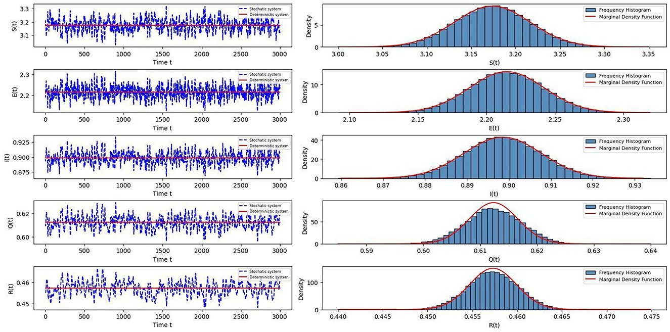
Figure 1. The left column shows persistent variations of S(t), E(t), I(t), Q(t), R(t) on deterministic Equation 2 and stochastic Equation 5, respectively. The right diagram gives the frequency histogram and marginal density function of the Equation 5.

Figure 2

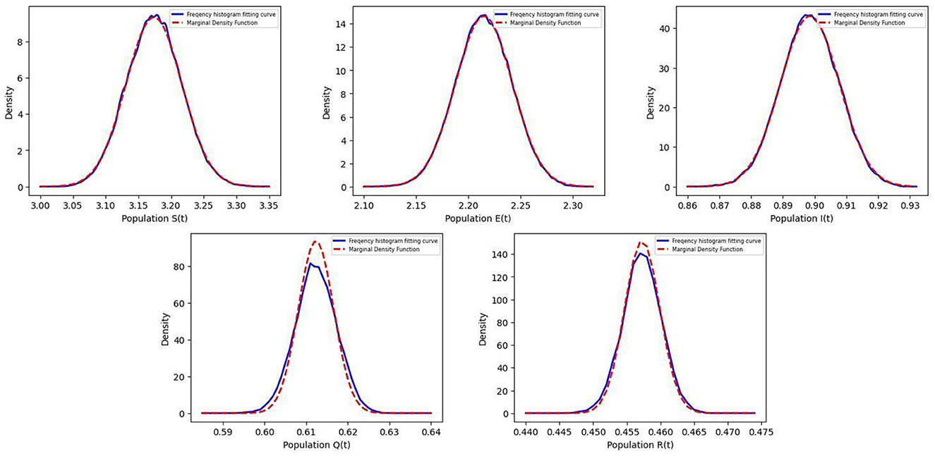
Figure 2. The figure shows the fitting curves of the frequency histogram and margin density function in the Equation 5.

Example 6.2 Choosing $\bar{\beta }=0.24$, α = 0.6, θ = 0.25, Λ = 0.6, δ = 0.16, ν = 0.28, γ = 0.2, σ₁ = 0.15, σ₂ = 0.032, ω₁ = 0.045, ω₂ = 0.06 and other parameters referring to Example 6.1, then we can calculate R₀ = 0.1617 < 1, $R_0^E=0.9512<1$ and there exists a disease-free equilibrium E₀ = (0.216, 0, 0, 0, 0) that is locally asymptotically stable. It is clearly shown in Figure 3 that the disease will become extinct over time.

Figure 3

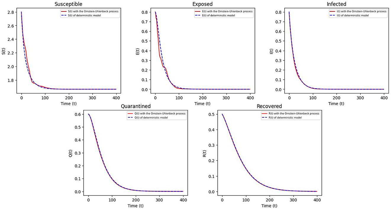
Figure 3. The trajectories of S(t), E(t), I(t), Q(t), R(t) in Equation 5 during the period of COVID-19 extinction.

Example 6.3 Taking three different values for the influence of volatility intensity θ:

$\begin{array}{l}\begin{array}{l}\theta =0.005,\theta =0.01,\theta =0.02.\end{array}\end{array}$

Let reversion speed α = 1.2, other parameters refer to Example 6.1. We can see that the smaller θ is, the smaller the fluctuation of the sample's trajectory is, and the more stable the disease is after observing the trajectories of S, E, I, Q, R in Figure 4.

Figure 4

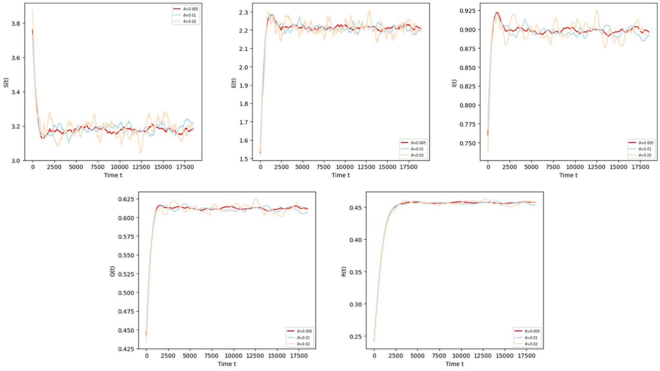
Figure 4. The trajectories of S(t), E(t), I(t), Q(t), R(t) in Equation 5 with different values for volatility intensity θ.

Example 6.4 To investigate the effect of reversion speed α on COVID-19 disease, take θ = 0.01 and other parameters refer to Example 6.1. Then, we choose three different values for reversion speed α:

$\begin{array}{l}\alpha =0.5,\alpha =0.8,\alpha =1.3.\end{array}$

From the sample trajectories of S, E, I, Q, R in Figure 5, the larger α is, the smaller the vibration of the sample motion trajectory is, and the more stable the disease is.

Figure 5

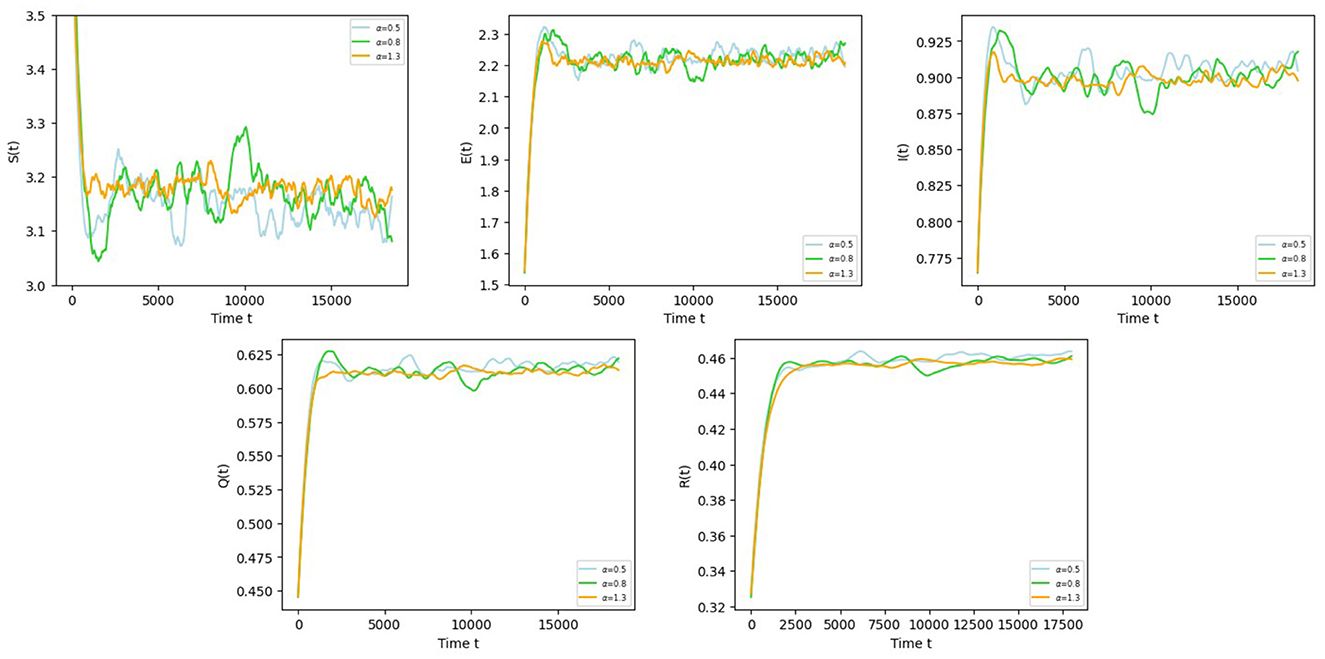
Figure 5. The trajectories of S(t), E(t), I(t), Q(t), R(t) in Equation 5 with different values for reversion speed α.

Example 6.5 In the following, we examine the impact of the Ornstein-Uhlenbeck process on the COVID-19 disease by modifying the parameter values of volatility intensity θ and reversion speed α in $R_0^S$ and $R_0^E$. For $R_0^S$, we choose θ ∈ [0.01, 0.3] and α ∈ [0.1, 1.5] and other parameters refer to example 6.1. For $R_0^E$, we choose θ ∈ [0.001, 0.04] and α ∈ [0.1, 2] and other parameters refer to example 6.2. As shown in Figure 6, as θ decreases and α increases, $R_0^S$ exhibits an increasing trend, which suggests that the disease will continue to exist in the future, while $R_0^E$ displays a decreasing trend, which indicates that the disease will tend to become extinct after a long time.

Figure 6

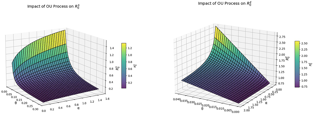
Figure 6. The graph on the left represents the trend of $R_0^S$ over the range (θ, α) ∈ [0.01, 0.3] × [0.1, 1.5]. The graph on the right side shows the trend of $R_0^E$ over the range (θ, α) ∈ [0.001, 0.04] × [0.1, 2].

7 Conclusion

This study investigates the dynamics of COVID-19 transmission with Ornstein-Uhlenbeck processes. Compared with the common linear combination of white noise, this study assumes that the transmission rate parameter β of the susceptible and exposed satisfies a mean-reversion process. This approach avoids the unbounded variance of β as the time step decreases and offers greater biological realism. In addition, taking into account the effect of transmission mechanisms, we introduced disease-caused mortality for I(t) and assumed that the disease-caused mortality rate h was greater than the natural mortality rate μ. For Equation 5, we first establish the existence and uniqueness of a global positive solution and prove its boundedness via the construction of a nonnegative Lyapunov-type function. On this basis we analyze the dynamical behavior of Equation 5 and derive the following key results:

(1) we fully utilize the ergodicity of the Ornstein-Uhlenbeck process to derive two critical values $R_0^S$ and $R_0^E$ related to disease persistence and extinction, where

$\begin{array}{l}{R}_0^S=\frac{\tilde{\beta }\Lambda \gamma }{(\delta +\mu )({\sigma }_1+{\omega }_1+\mu +h)({\sigma }_2+\gamma +\nu +\mu +c_1\frac{\Lambda \theta }{\mu \sqrt{\pi \alpha }})},\\ R_0^E=\sqrt{R_0}+\\ \frac{\gamma \theta \Lambda }{\mu ({\sigma }_2+\gamma +\nu +\mu )\sqrt{R_0\pi \alpha }min\left\{{\sigma }_2+\gamma +\nu +\mu ,{\sigma }_1+{\omega }_1+\mu +h\right\}}.\end{array}$

When $R_0^S>1$, it indicates that the stochastic system has a stationary distribution, meaning that the disease will persist over time. To further determine the size relationship between $R_0^S$ and R₀, we define an $R_{00}^S$ such that $R_{00}^S\le R_0^S$ and $R_{00}^S\le R_0$. It follows that when $R_{00}^S>1$ there is $R_0^S>1$ and R₀>1. This suggests that $R_{00}^S>1$ can be considered as a harmonized threshold for disease prevalence for both deterministic and stochastic systems.

When $R_0^E<1$ indicates that the disease will become extinct over time. And $R_0^E<1$ can derive R₀ < 1. This shows that $R_0^E<1$ can be regarded as a unifying condition for deterministic and stochastic models of disease extinction.

(2) To further investigate the dynamical behavior of the disease, a display expression for the probability density function in the quasi-equilibrium nearby was derived by solving the sixth-order Fokker–Planck Equation 28. And we draw an image of the probability density function as shown in Figure 1.

(3) We verify our theoretical results with numerical simulations and find that both larger fluctuation intensity and smaller speed of regression may lead to extinction of the disease.

This study proposes a stochastic SEIRQV model incorporating an Ornstein-Uhlenbeck process. By introducing a quarantine compartment, the model comprehensively accounts for the combined effects of vaccination and quarantine measures on the transmission of infectious diseases. To evaluate model performance and the effectiveness of isolation measures, we conducted a comparative analysis of simulation results against an existing stochastic SEIV model [22]. Our findings suggest that integrating natural mortality rates with artificial isolation policies enhances our model's precision in estimating disease extinction probabilities and steady-state distributions. The interaction between isolation and other compartments generates a modified critical threshold condition, more accurately reflecting the impact of combined intervention measures. Compared with existing stochastic SEIR models [23], this model captures richer covariance structures across all compartments. Moreover, the variance and covariance terms explicitly depend on isolation and vaccination rates, which provides a stronger theoretical basis for evaluating the variability and potential outcomes of disease control strategies.

In summary, our study presents a more realistic stochastic model that overcomes the limitations of the white noise model in simulating the dynamics of COVID-19 infection. Although we have made a breakthrough in this aspect, we still need to exploit other valid approaches to compensate for the limitations of the study. For example, further explore harmonized thresholds for disease persistence and extinction, find a more suitable method and theory to determine the uniqueness of the stationary distribution, consider incorporating more compartmental models into COVID-19 infectious disease research, and integrate age structures to study differences in susceptibility and contact patterns across age groups.

Data availability statement

The original contributions presented in the study are included in the article/supplementary material, further inquiries can be directed to the corresponding author.

Author contributions

W-HL: Writing – review & editing. K-JW: Writing – original draft, Writing – review & editing.

Funding

The author(s) declare that financial support was received for the research and/or publication of this article. This work was supported by the National Natural Science Foundation of China (Grant No.:52474035) and the Heilongjiang Provincial Postdoctoral Science Foundation (LBH-Z23259).

Acknowledgments

The authors gratefully acknowledge the Heilongjiang Provincial Postdoctoral Science Foundation (LBH-Z23259).

Conflict of interest

The authors declare that the research was conducted in the absence of any commercial or financial relationships that could be construed as a potential conflict of interest.

Generative AI statement

The author(s) declare that no Gen AI was used in the creation of this manuscript.

Any alternative text (alt text) provided alongside figures in this article has been generated by Frontiers with the support of artificial intelligence and reasonable efforts have been made to ensure accuracy, including review by the authors wherever possible. If you identify any issues, please contact us.

Publisher's note

All claims expressed in this article are solely those of the authors and do not necessarily represent those of their affiliated organizations, or those of the publisher, the editors and the reviewers. Any product that may be evaluated in this article, or claim that may be made by its manufacturer, is not guaranteed or endorsed by the publisher.

Supplementary material

The Supplementary Material for this article can be found online at: https://www.frontiersin.org/articles/10.3389/fams.2025.1687991/full#supplementary-material

References

1. She J, Jiang J, Ye L, Hu L, Bai C, Song Y, et al. 2019 novel coronavirus of pneumonia in Wuhan, China: emerging attack and management strategies. Clin Transl Med. (2020) 9:1–7. doi: 10.1186/s40169-020-00271-z

PubMed Abstract | Crossref Full Text | Google Scholar

2. Cucinotta D, Vanelli M. WHO declares COVID-19 a pandemic. Acta Biomed. (2020) 91:157. doi: 10.23750/abm.v91i1.9397

PubMed Abstract | Crossref Full Text | Google Scholar

3. Kaur SP, Gupta V. COVID-19 vaccine: a comprehensive status report. Virus Res. (2020) 288:198114. doi: 10.1016/j.virusres.2020.198114

PubMed Abstract | Crossref Full Text | Google Scholar

4. Tang B, Wang X, Li Q, Bragazzi LN, Tang S, Xiao Y, et al. Estimation of the transmission risk of the 2019-nCoV and its implication for public health interventions. J Clin Med. (2020) 9:462. doi: 10.3390/jcm9020462

PubMed Abstract | Crossref Full Text | Google Scholar

5. Poonia RC, Saudagar AKJ, Altameem A, Alkhathami M, Khan MB, Hasanat MHA, et al. An enhanced SEIR model for prediction of COVID-19 with vaccination effect. Life. (2022) 12:647. doi: 10.3390/life12050647

PubMed Abstract | Crossref Full Text | Google Scholar

6. Fosu GO, Opong JM, Appati JK. Construction of compartmental models for COVID-19 with quarantine, lockdown and vaccine interventions. SSRN Electronic J. (2020). doi: 10.2139/ssrn.3574020

PubMed Abstract | Crossref Full Text | Google Scholar

7. Yang Q, Zhang X, Jiang D. Dynamical behaviors of a stochastic food chain system with Ornstein–Uhlenbeck process. J Nonlinear Sci. (2022) 32:34. doi: 10.1007/s00332-022-09796-8

PubMed Abstract | Crossref Full Text | Google Scholar

8. Shi Z, Jiang D. Dynamics and density function of a stochastic COVID-19 epidemic model with Ornstein–Uhlenbeck process. Nonlinear Dyn. (2023) 111:18559–84. doi: 10.1007/s11071-023-08790-3

Crossref Full Text | Google Scholar

9. Su X, Zhang X, Jiang D. Dynamics of a stochastic HBV infection model with general incidence rate, cell-to-cell transmission, immune response and Ornstein–Uhlenbeck process. Chaos Solitons Fractals. (2024) 186:115208. doi: 10.1016/j.chaos.2024.115208

Crossref Full Text | Google Scholar

10. Zhang XA. stochastic non-autonomous chemostat model with mean-reverting Ornstein–Uhlenbeck process on the washout rate. J Dyn Differ Equ. (2024) 36:1819–49. doi: 10.1007/s10884-022-10181-y

Crossref Full Text | Google Scholar

11. Liu Q, Jiang D. Stationary distribution and probability density for a stochastic SEIR-type model of coronavirus (COVID-19) with asymptomatic carriers. Chaos, Solitons Fractals. (2023) 169:113256. doi: 10.1016/j.chaos.2023.113256

PubMed Abstract | Crossref Full Text | Google Scholar

12. Shi Z, Jiang D, Zhang X, Alsaedi A. A stochastic SEIRS rabies model with population dispersal: stationary distribution and probability density function. Appl Math Comput. (2022) 427:127189. doi: 10.1016/j.amc.2022.127189

Crossref Full Text | Google Scholar

13. Wei S, Jiang D, Zhou Y. Dynamic behavior of a stochastic HIV model with latent infection and Ornstein–Uhlenbeck process. Math Comput Simul. (2024) 225:731–59. doi: 10.1016/j.matcom.2024.06.011

Crossref Full Text | Google Scholar

14. Liu Y, Wang Y, Jiang D. Dynamic behaviors of a stochastic virus infection model with Beddington–DeAngelis incidence function, eclipse-stage and Ornstein–Uhlenbeck process. Math Biosci. (2024) 369:109154. doi: 10.1016/j.mbs.2024.109154

PubMed Abstract | Crossref Full Text | Google Scholar

15. Allen E. Environmental variability and mean-reverting processes. Discrete ContinDynSyst SerB. (2016) 21:2073–89. doi: 10.3934/dcdsb.2016037

Crossref Full Text | Google Scholar

16. Du NH, Nguyen DH, Yin GG. Conditions for permanence and ergodicity of certain stochastic predator–prey models. J Appl Probab. (2016) 53:187–202. doi: 10.1017/jpr.2015.18

Crossref Full Text | Google Scholar

17. Meyn SP, Tweedie RL. Stability of Markovian processes III: Foster–Lyapunov criteria for continuous-time processes. Adv Appl Probab. (1993) 25:518–48. doi: 10.2307/1427522

Crossref Full Text | Google Scholar

18. Dieu NT. Asymptotic properties of a stochastic SIR epidemic model with Beddington–DeAngelis incidence rate. J Dyn Differ Equ. (2018) 30:93–106. doi: 10.1007/s10884-016-9532-8

Crossref Full Text | Google Scholar

19. Cai Y, Jiao J, Gui Z, Liu Y, Wang W. Environmental variability in a stochastic epidemic model. Appl Math Comput. (2018) 329:210–26. doi: 10.1016/j.amc.2018.02.009

Crossref Full Text | Google Scholar

20. Zhang X, Yuan RA. stochastic chemostat model with mean-reverting Ornstein-Uhlenbeck process and Monod-Haldane response function. Appl Math Comput. (2021) 394:125833. doi: 10.1016/j.amc.2020.125833

Crossref Full Text | Google Scholar

21. Roozen H. An asymptotic solution to a two-dimensional exit problem arising in population dynamics. SIAM J Appl Math. (1989) 49:1793–810. doi: 10.1137/0149110

Crossref Full Text | Google Scholar

22. Su T, Yang Q, Zhang X, Jiang D. Stationary distribution, extinction and probability density function of a stochastic SEIV epidemic model with general incidence and Ornstein–Uhlenbeck process. Phys A: Stat Mech Appl. (2023) 615:128605. doi: 10.1016/j.physa.2023.128605

Crossref Full Text | Google Scholar

23. Lu C, Xu C. Dynamic properties for a stochastic SEIR model with Ornstein–Uhlenbeck process. Math Comput Simul. (2024) 216:288–300. doi: 10.1016/j.matcom.2023.09.020

PubMed Abstract | Crossref Full Text | Google Scholar