Financing the Transition Toward Carbon Neutrality—an Agent-Based Approach to Modeling Investment Decisions in the Electricity System

Introduction

Global CO₂ emissions from power generation have increased continuously from 7.6 Gt CO₂ in 1990 to around 14 Gt CO₂ in 2018 as a result of fossil fuel combustion (IEA, 2020). In order to reach the internationally agreed climate goals, it is critical to rapidly shift from fossil fuels to low-carbon technologies for power production.

Meeting climate goals requires mobilizing large amounts of investments to low-carbon technologies (FS-UNEP and BNEF, 2019; IRENA, 2020a). Despite the fact that global investments in new renewable capacity have grown significantly, the International Renewable Energy Agency (IRENA) has estimated that to meet the 1.5-degree target, the current annual investment in renewables has to be at least doubled in the 2016–2050 period (IRENA, 2020b). However, as energy projects are typically capital intensive, with long pay-back periods, financing investments can be challenging, blocking the transition. This suggests a need for a better understanding of the energy transition from the perspective of financial factors such as accessibility to, risks and costs of, and returns on, capital, in order to assess how these factors impact investment choices and transition pace.

When studying the energy transition, a wide range of computational models have been employed for assessing the feasibility and consequences of different investment options in light of the climate goals, for example, TIMES (Loulou et al., 2005), GET (Azar et al., 2003, 2013), E3ME (Econometrics, 2019), NEMS (EIA, 2019), PRIMES (NTUA and EMI, 2014), PowerAce (Genoese, 2010), EMLab (Chappin et al., 2017), etc. These models are useful as they may help decision-makers understand the potential consequences of various policy proposals and make wise decisions.

However, not all types of models are suitable for better understanding how energy investments are made and financed in a realistic way or for elucidating how individual investment decisions affect the overall system and vice versa. For example, in optimisation models, there is normally a “central decision-maker” who assures all necessary investments will be made so that the least-cost solution of the model is reached. In addition, neither general equilibrium models nor macroeconomic models are, in their current forms, well-equipped to assess important financial and macroeconomic impacts such as bankruptcies, stranded assets, and debt defaults (Pollitt and Mercure, 2018).

A recent paper published in Science highlights the importance of including the financial system (and investors' decisions) in the Integrated Assessment Models (IAMs) (Battiston et al., 2021). This study points out that IAMs assume companies have access to capital at no cost and do not take into account the different levels of risk aversion of investors, and this could distort the results of costs and benefits of climate mitigation policies, and therefore, argues that to better inform policy and investment decisions, the feedback loop between the financial system and mitigation pathways should be taken into account in the (IAM) models.

Agent-based models (ABMs), on the other hand, are able to reproduce many stylised facts of modern economies and capture the financial activity (Pollitt and Mercure, 2018). Previous studies have demonstrated that ABMs are capable of explicitly representing the financing mechanism of investments (in the power sector). For example, their ABM models Gerst et al. (2013) and Ponta et al. (2018) have applied the “pecking order theory,” which says that when financing a project, firms prefer to use internal funds first, and if internal funds are inadequate, then external debt is issued, and external equity is used as the last resort (Myers and Majluf, 1984). Other models put constraints on access to loans. One example is the BRAIN-Energy model (Barazza and Strachan, 2020), in which the authors have implemented a limit on the amount of capital an agent can borrow from the bank, with the interest rate depending on the type of agent. This means that an agent must cover part of each investment cost using its own financial means, and then paying back loans in installments.

Some ABMs have implemented mechanisms that reflect how a company's previous profits impact its ability to finance future investments. For example, Safarzynska and van den Bergh (2017) implemented the debt-to-equity ratio of a company as the criterion for whether the company can get a loan from a bank to finance an investment. Another example is Kraan et al. (2018), who implemented an adaptive discount method in their ABM, where the agent goes bankrupt if its discount rate rises above a given threshold.

In our previous work, we have developed an agent-based model for an electricity system and studied the system transition toward a low-carbon future (Jonson et al., 2020; Yang et al., 2021). We focused on investment decisions by agents that had limited foresight about future carbon, fuel, and electricity prices and that applied varying hurdle rates in their investment analysis.

In this study, we present the HAPPI (Heterogenous Agent-based Power Plant Investments) model, which is an extension of the previous ABM with a financial feedback module that includes agent-specific details of economic components. We keep track of each agent's investment decisions, equity, cash flow, investment return, and dividend. This extension enables us to study the impact of different financial constraints that the companies face.

The overall aim of this paper is to study the transition toward a low carbon future using our HAPPI model, while paying particular attention to the financial flows of each agent. More specifically, this paper aims to:

1. Introduce the financial module in our ABM and analyse how the financing constraint and capital availability impact a company's investment decisions and economic performance and, in turn, the transition toward a low carbon future.

2. Investigate, under different levels of financial constraints and capital availabilities, which investment criteria, in terms of different levels of expectation of future carbon price and in terms of how risk averse companies are, more robustly avoids (or reduces the risk of) bankruptcy while guaranteeing a certain level of profitability.

In section Model description, we describe our model, focussing on the development of the financial module, and in section Set-up of the experiment, we present the different cases we investigate. In sections Results and Sensitivity analysis we present model results and sensitivity analysis. We conclude with the discussion in section Conclusion.

Model Description

Basic Model Description

The HAPPI model consists of agents that are power companies (in the rest of this paper, we use “agent” and “company” interchangeably). They invest in new capacity and produce electricity in an ideal electricity market. There are six types of power plants in which an agent can choose to invest: coal-fired, gas-fired, gas-fired with CCS (gasCCS), nuclear, wind and solar PV power plants (see Supplementary Table 1 for parameter settings of power plants). The gas-fired plant can be fuelled by natural gas or biogas, depending on which has the lower operating cost when the carbon tax is also taken into account.

Each year, plants that reach the end of their lifetime are retired, and all agents evaluate all investment options and invest in the plants with the highest expected profits. Agents take turns making investment decisions; the order is randomized.

In our current model version, agents are heterogeneous in two attributes. The first attribute is the hurdle rate that an agent employs, which reflects that agent's risk management strategy. The set of hurdle rates is [4.5%, 5%, 6%, 8%] per year. The hurdle rate is chosen based on several studies. For example, IEA reports the weighted average cost of capital (WACC) for major power companies was around 8%/year in 2006 and dropped to around 5%/year in 2018 (IEA, 2019); IRENA reports that the WACC is 7.5%/year for OECD countries and China, and 10%/year for the rest of the world (IRENA, 2018). An EU study reports that WACC varied across the EU Member States from 3.5%/year in Germany to 12%/year in Greece for onshore wind projects in 2014 (DiaCore, 2016). The National Energy Modeling System (NEMS) of the US Energy Information Administration uses 6–7%/year in its WACC estimation (EIA, 2020).

The second attribute is the agent's expectation of future carbon prices. Agents have limited information about future carbon prices. They know the true carbon tax of next year, and they estimate the tax level 10 years ahead. Their expectation on the future tax (at time t + 10), denoted F_b(t+10), is given by the tax in the next year T(t+1) plus a factor b times the difference between the true tax T(t+10) in 10 years time and the tax in next year,

$\begin{array}{ll}\begin{array}{c}{F}_b(t+10)=T(t+1)+b(T(t+10)-T(t+1))\\ \end{array}& (1)\end{array}$

We use a set [0, 0.5, 1.0, 1.5, 2.0] for b, which means that agents' expectations on the rate at which the tax will increase range from no increase to twice as high as the actual rate.

All combinations of the two attributes—hurdle rate r and expectation parameter b–are possible, so there are 20 different agents active in the electricity system.

Agents generate revenue by selling electricity from the plants they own. A plant generates power as long as the electricity price is greater than or equal to the running cost of that plant. The electricity price is determined by an iso-elastic demand function (see Supplementary Equation 1). In order to capture the variability of demand, wind, and solar, we divide each year into 64 slices with different numbers of hours. This means that electricity price and production are calculated 64 times per year (see Supplementary Table 2 for time slicing).

Model Development

Financial Feedback Module

We have extended our basic model with a financial feedback module. This module keeps track of each agent's financial status, and this in turn is used to determine whether an agent can afford to make further investments.

We use the following mechanism in our approach: First, an agent is assumed to supply a certain fraction f of any new investment from its own bank account; the remaining part of the investment, (1−f), is paid by a loan from the bank with an interest rate l. In the present version of the model, if the agent cannot afford the payment to invest in the top NPV-ranked power plant, then it will not invest in the current round. Second, the own bank account can accumulate profit from the company's plant operations and a certain fraction f_div of the capital can be paid to shareholders as dividend d, provided that the planned investments for coming years can be made, as described below. There is no interest on the own bank account, but if the balance on the account is negative, this is regarded as an ordinary loan with interest l.

We add the following variables characterizing the state of a company and the requirements for new investments:

1. The equity E of a company in our model is defined as the total value of its plants, V, plus the bank account holdings M minus its debt D to the bank. If the equity goes below zero, the company is bankrupt.

$\begin{array}{ll}\begin{array}{c}E=M+V-D\\ \end{array}& (2)\end{array}$

2. From 1 year to the next, the money in the bank account changes due to net revenues R_net (defined as revenues from selling electricity less operating costs), investment costs I, interest costs C_{l, f}, repayment of loans L_{l, f}, and dividend d paid to shareholders,

$\begin{array}{l}M(t+1)-M(t)=\\ R_{net}(t)-f·I(t)-C_{l,f}(t)-L_{l,f}(t)-d(t)& (3)\end{array}$

Note that, together, C_{l, f} and L_{l, f} are given by (1−f)A_l, where A_l is the sum of all annualized costs of the standing plants, since the fraction (1−f) of an investment is financed by borrowing. Similarly, investment costs f·I are a fraction of full investment costs, where I is the sum of full investment cost for plants in a specific year. A company is not allowed to invest if the money in the bank account goes below zero ahead of that year's investment round.

The dividend d is paid according to the following rules:

a. First, investments are made according to the company's rules of operation.

b. A given amount m_save is reserved to allow for a future (hypothetical) investment in the most expensive plant. This means that dividends are not generally paid and especially not in the initial years when the companies are in a growth phase.

c. Up to a fraction f_div of the money in the bank account is paid to the shareholders as a dividend, but not more than so that m_save is kept, i.e., d = Min(f_divM, M−m_save ).

3. The total value of a company's plants, V, changes due to new investments I and capital depreciation of plants, C_depr,

$\begin{array}{ll}\begin{array}{c}V(t+1)-V(t)=I(t)-C_{depr}(t)\\ \end{array}& (4)\end{array}$

Each plant has a value V_plant that initially is equal to its investment cost and then equals the remaining debt that one would have if one were (hypothetically) to have borrowed the funds for the full investment at a loan interest l and paid the annualized capital cost every year. The value V_plant(t_R) of the plant with a remaining lifetime t_R can then be expressed as

$\begin{array}{ll}\begin{array}{c}{V}_{plant}(t_R)=I_{plant}\frac{1-{(1+r_l)}^{-t_R}}{1-{(1+r_l)}^{-t_L}}\\ \end{array}& (5)\end{array}$

where I_plant is the plant investment cost and t_L is the full lifetime.

4. The debt D changes due to new loans taken and repayment of present loans L_{l, f}. New loans are taken to cover (1−f) of investment costs, so the change in debt is then

$\begin{array}{ll}\begin{array}{c}D(t+1)-D(t)=(1-f)I(t)-L_{l,f}(t)\\ \end{array}& (6)\end{array}$

5. By combining Equations (2–4, 6), we get the change in equity

$\begin{array}{ll}\begin{array}{c}E(t+1)-E(t)=R_{net}(t)-C_{l,f}(t)-C_{depr}(t)-d(t)\\ \end{array}& (7)\end{array}$

Note that since we give a value of the plants according to Equation (5), the capital depreciation equals the repayment of a hypothetical loan for full investment costs.

Evaluation of Economic Performance

The economic performance is investigated ex-post both for individual investments and individual companies. For the individual investments, we use the internal rate of return (IRR), which is the discount rate that makes the net present value of all cash flows (including the investment cost) during the lifetime t_L of a project equal to zero (see Equation 7). This gives a measure of the economic return on investment. The IRR is then the solution to the equation

$\begin{array}{ll}\begin{array}{c}0={\displaystyle {\sum }_{t=1}^{t_L}}\frac{r_t-c_t}{{(1+IRR)}^t}-I_{plant}\\ \end{array}& (8)\end{array}$

where r_t and c_t are the revenues and operating costs in year t, and I_plant is the investment cost of the plant.

In real life, when assessing the economic performance of a company, several measures are used, e.g., profit, return on equity (ROE), return on capital employed (ROCE), and equity ratio (i.e., equity divided by company's total assets as a measure of indebtedness). In this paper, we will focus on return on equity. It is a measure of the return an investor may get from investing in the company. It should be noted that this can be significantly higher than the return on a particular investment project, since the investment in the project can be financed with borrowed money. Here we use the return on equity ROE given by net revenues R_net (revenues from selling electricity less operating costs) less interest C_{l, f} and depreciation costs C_depr divided by equity E,

$\begin{array}{ll}\begin{array}{c}ROE=\frac{R_{net}-C_{l,f}-C_{depr}}{E}\\ \end{array}& (9)\end{array}$

i.e., net profit divided by equity. In case there is no dividend paid, R_net−C_{l, f}−C_depr is the change in equity from 1 year to the next, see Equation (7). ROE thus quantifies the equity growth (before the dividend is paid).

We also evaluate an individual company's performance by its bankruptcy risk. We run the model multiple times under different settings that reflect different levels of financing constraints and access to capital (see section Set-up of the experiment, below) and we measure the frequency with which an agent goes bankrupt (equity goes below zero) as an indicator of economic risk. (A model description following the ODD (Overview, Design concepts, and Details) protocol can be found online at https://github.com/happiABM/HAPPI/blob/main/ODD-HAPPI_model_description.docx).

Set-Up of the Experiment

Model Settings

Initial Capacity

For the present work, the model starts with a stationary state with 64 GW coal and 2 GW gas in the system.¹ Since we focus on the decisions made by companies and the effect of the financial feedback, we separate the initial coal and gas plants from the analysis, and they are all placed in an additional separate company that will not take part in the investment process, but that will run the plants throughout their lifetime.

Carbon Tax

We assume that the CO₂ tax stays at 0 for the first 10 years and then grows linearly by 2€/ton per year to 100 €/ton at year 60 and stays at 100 €/ton per ton thereafter (We also test different tax scenarios, see the sensitivity analysis in section Sensitivity analysis).

Experimental Design

We first set up two experiments to test two variables,

1) f : the fraction of an investment financed by a company's own capital.

2) i: the initial capital (M€) in a company's bank account.

These tests allow us to investigate how various financial constraints and capital availabilities may affect agents' investment options, and how this in turn affects the overall transition to a low-carbon electricity system.

In order to compare different cases, we use a base case as the reference, where we set f = 30%, i = 400 M, and there is no stochasticity in fuel price or electricity demand. In all cases, the bank interest rate l is set to 4%/year, the reserved amount m_save is 1,500 M€, and the dividend fraction f_div is 50%.

Experiment 1: Varying f

We test six cases of parameter f (investment fraction financed by a company's capital), where f ϵ [0, 10, 20, 30, 40, 50%]. According to the IEA, the debt to equity ratio is 50:50 (IEA, 2019), whereas another study by FS-UNEP reports 60:40 to 80:20 (FS-UNEP and BNEF, 2020). The initial capital is set at the reference level (i = 400 M€).

Experiment 2: Varying i

We test five levels for the initial capital in a company's bank account i ϵ [225²,400, 900, 1,200, 2,000] M€. The fraction f is set at its reference level (f = 30%).

Results

Results for the Base Case

System Level

Aggregate Capacity

In the scenario with an increasing carbon tax, the system transits from a coal- and gas-based to a low-carbon electricity system (Figure 1); meanwhile, CO₂ emissions drop continuously (Figure 2). The wind is the first low-carbon technology that starts to expand, followed by the gas-fired power plants (first used with natural gas and then used with biogas, or with natural gas and CCS), solar PV, and nuclear power plants. The capacity of wind drops after around year 40 due to competition from nuclear.

FIGURE 1

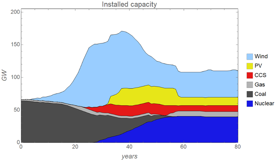
Figure 1. System installed capacity from year 0 to year 80 in the base case [f = 30% and i = 400M€. f is the fraction of an investment financed by a company's own capital and i is the initial capital in a company's bank account].

FIGURE 2

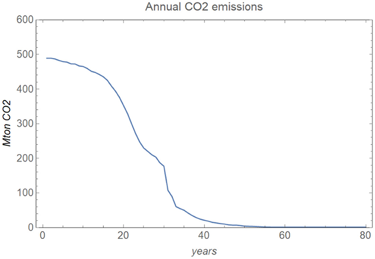
Figure 2. Emissions in the base case [f = 30% and i = 400M€. f is the fraction of an investment financed by a company's own capital and i is the initial capital in a company's bank account].

It is interesting to observe that nuclear power eventually comes to take a large market share from wind even though the levelized cost of wind is lower than that of nuclear. This can be understood in the following way. First, when the carbon tax increases, electricity prices go up and the wind starts to expand. However, when the carbon tax is so high that coal is phased out, electricity prices start to increase substantially when wind output is low. This provides the incentive for investments in nuclear power, and when nuclear power expands significantly, it tends to be used most of the time (capital costs are high, running costs are low), and this offers a downward pressure on the electricity price throughout the year, which in turn reduces the profitability for wind. In non-economic terms, one can say that it is the fact that nuclear can provide electricity essentially all the time whereas wind turbines only provide electricity under windy conditions that gives nuclear the advantage over wind. The factors that play here are of course more complex given that there are also gas-fired power plants that can be used with natural gas or biogas, as well as natural gas with CCS and solar PV. For instance, assuming lower costs for biogas implies that biogas cost-effectively can act as a complement to wind and the electricity system that would strongly benefit the combination of wind and biogas at the expense of nuclear (Sepulveda et al., 2018; Yang et al., 2021).

CO₂ Emissions

In Figure 2, we can see that CO₂ emissions are reduced by half after about 25 years, when the CO₂ tax has reached 30€/ton CO₂. The emissions are then further reduced to almost zero after 40–50 years (this is 30–40 years after the tax was implemented in the model). This is a rapid reduction, but it is roughly in line with the Paris agreement targets, as well as the CO₂ net-zero emission targets adopted by the EU for 2050, and it illustrates the rapid transition required.

Internal Rate of Return

Figure 3 shows the ex-post analysis of the internal rate of return (IRR) of each investment made for each year. During the early phase of the transition (around year 10–30), coal plants gradually become unprofitable because of the increasing carbon tax. Meanwhile, investments made in gas and gasCCS plants also result in losses, while investments in the wind are quite profitable, yielding returns as high as more than 5%/yr.

FIGURE 3

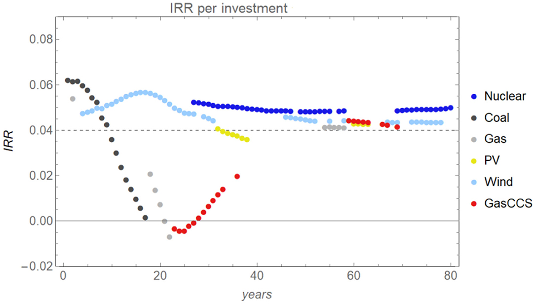
Figure 3. Internal rate of return (IRR) in the base case [f = 30% and i = 400M€. f is the fraction of an investment financed by a company's own capital and i is the initial capital in a company's bank account]. Each dot indicates the IRR of an investment made in a particular year. The horizontal dash line indicates the 4% bank interest rate.

Later (around year 30–60), companies start to invest in nuclear, and IRRs of different technologies converge closely to around 4–5%/year, which means the return on wind drops during this period while investments in gas-fired power plants become profitable (after switching to biofuels).

At the end of the simulation period (after year 60), IRRs remain around 4–5%/year, which is the hurdle rate employed by the agents making most of the investments during this period (see Figures 4, 5 below); this means that these dominant agents receive returns roughly in line with what they expected (agents with a hurdle rate of 6% or more will get less than what they expected). Note that for an investment to break even, its IRR can be lower than the 4% bank interest rate, since part of the funding for the project came from the company's own capital.

FIGURE 4

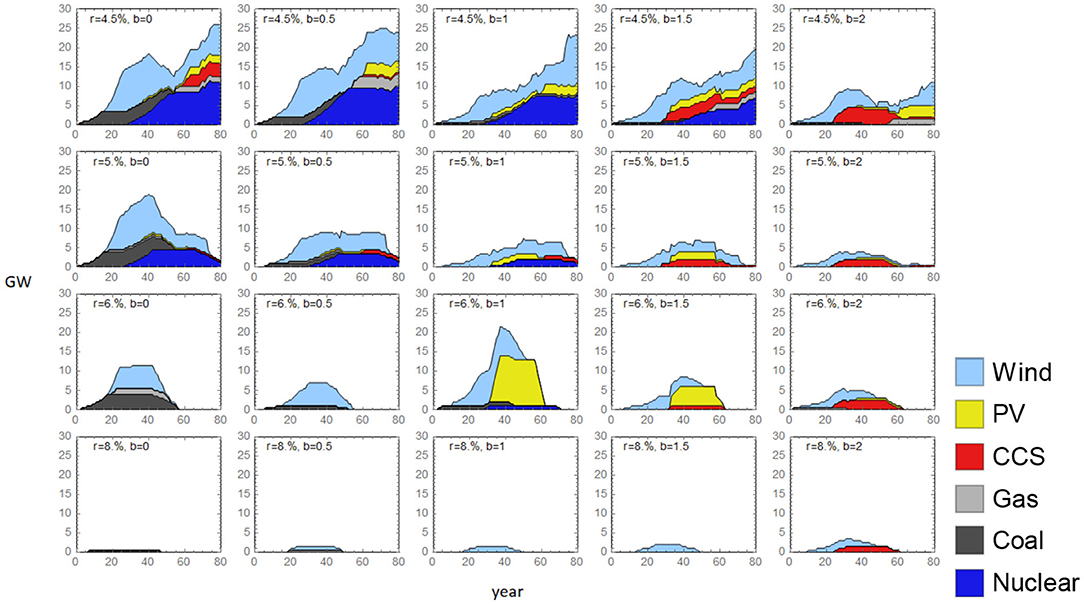
Figure 4. Installed capacity of 20 individual agents in the base case [f = 30% and i = 400M€. f is the fraction of an investment financed by a company's own capital and i is the initial capital in a company's bank account]. r is the hurdle rate agents use and b is the expected carbon tax parameter.

FIGURE 5

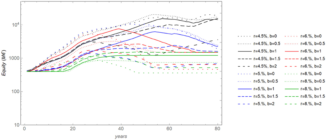
Figure 5. Equity for the 20 companies in a base case run [f = 30% and i = 400M€. f is the fraction of an investment financed by a company's own capital and i is the initial capital in a company's bank account]. Companies with lower hurdle rates r dominate, except those that expect the highest carbon tax, i.e., have the greatest expectation parameter b. Companies that have accurate tax expectations perform well in this perspective for all hurdle rates.

On the Level of Individual Agents

Investment Decisions

When we look at the installed capacity on the agent level, we see that agents with different attributes (hurdle rates r and expectations of future carbon prices b) invest differently. Figure 4 illustrates that, firstly, in general, agents with relatively low hurdle rates (r = 4.5%/yr and r = 5%/yr) are more willing to invest, while agents with a high hurdle rate (r = 8%/yr) rarely make investments. This is because agents using lower hurdle rates require a lower return on their investments. Investments from these agents lower the overall electricity prices and crowd out other agents that require a higher return on investments.

Secondly, agents that expect low carbon prices (b = 0) invest heavily in coal power plants in the beginning³, whereas agents expecting high carbon prices (b = 1.5 and b = 2) take earlier action investing in wind and gasCCS plants, but gasCCS investments turn out to be unprofitable (see Figure 3). Agents that expect a more correct carbon price (b = 1) stop investing in coal, shifting investments to wind in a timely manner.

Return on Equity

When assessing agents based on their return on equity, the agents who apply low hurdle rates (r = 4.5% and 5% per year) and have a more accurate expectation for the carbon price (b = 0.5 or 1.0) are those that perform well, in general. See Figure 5 where we plot the development of equity over time and Figure 6 for the annual return on equity for all agents. Figure 7 shows the average ROE for a 10-year period in the expansion phase (years 30–40). The average ROE is obtained from the geometric average of the factors (1 + ROE) that contribute to the equity growth for the included years, with a correction for dividends paid (in case that happens, which is rare in the expansion phase). For details of this calculation, see Supplementary Equation 2.

FIGURE 6

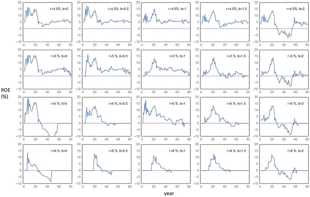
Figure 6. Return on equity (ROE) for all companies over the full-time period of 80 years in the base case [f = 30% and i = 400M€]. f is the fraction of an investment financed by a company's own capital and i is the initial capital in a company's bank account. r is the hurdle rate agents use and b is the expected carbon tax parameter.

FIGURE 7

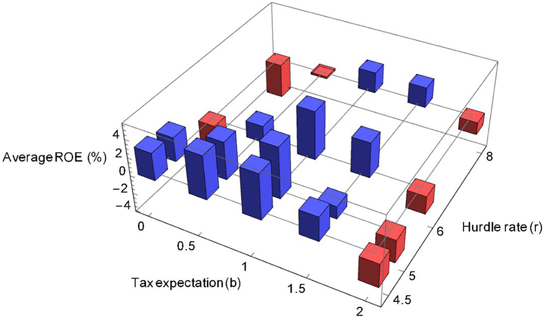
Figure 7. The average ROE over a 10-year period for the 20 agents during the expansion phase from year 30 to 40. Positive and negative values are depicted by blue and red, respectively. Companies with more accurate expectations on tax changes perform better during this period. In the base case, we use f = 30% and i = 400M€. f is the fraction of an investment financed by a company's own capital and i is the initial capital in a company's bank account.

These more successful agents mainly invest in the wind early on (around year 10–20) and accumulate profits from these investments. They then move on to invest in nuclear and PV. Later, around year 60, they also invest in gas-fired power plants (used with biogas) and natural gas with CCS (see Figure 4).

Exploring the Impact of Financial Constraints and Capital Availability

In this section, we explore how financial constraint and capital availability affect agents' investment decisions and performances, which in turn affects the aggregate capacity mix and the pace of emission reductions.

On the System Level–Capacity and CO₂ Emissions

At the system level, we observe that different capital availability levels and financing constraints result in different development paths of the overall capacity mix (Figure 8). In the left column, we vary the investment fraction f that has to be paid from a company's bank account, and in the right column, we vary the initial capital i of the company. With a more stringent access to capital (i.e., for higher values of f or lower values of i), the coal phase-out is slower and there is a delay in investments in low-carbon technologies such as wind, nuclear, and PV. This is because wind, nuclear, and PV have high investment costs, and since agents lack capital, especially during the early phases of the transition period, these investments become more difficult with less access to capital.

FIGURE 8

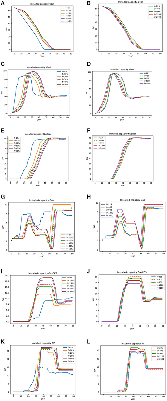
Figure 8. Installed capacity in cases with different capital accessibilities. (A,B) Coal; (C,D) wind; (E,F) nuclear; (G,H) gas; (I,J) gasCCS; (K,L) solar PV. “f” is the fraction of an investment financed by a company's own capital and “i” is the initial capital in a company's bank account. Dashed line is the base case.

Due to the delayed shift to low-carbon investing, CO₂ emission reductions also slow down when agents have less access to capital (Figure 9).

FIGURE 9

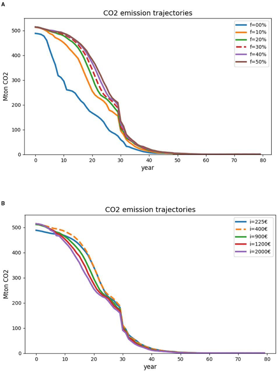
Figure 9. Emission trajectories in cases with different levels of capital accessibility. (A) cases with varying f, which is the fraction of an investment financed by a company's own capital; (B) cases with varying i, which is the initial capital in a company's bank account. The dashed line represents the base case (f = 30% and i = 400M€).

Despite capacity mix development paths differing among cases (during the transient phase), the mix reaches similar levels in the end across all these cases. This is because the (successful) agents (with low hurdle rates) become less capital-constrained over time, and the carbon tax stabilizes after year 60.

On the Level of Individual Agents

Investments

Results show that an agent's capacity mix varies with different levels of access to capital (fand i). Overall, we observe that first, when agents are required to finance the project with a very low ratio from their own bank account (i.e., f = 0 or 10%), the overall investment is dominated by the few agents who apply low hurdle rates, while when a higher f ratio is required, investments are more evenly distributed among agents (see Supplementary Figures 1, 2, where cases of f = 10% and f = 50% are presented). This is because the greater f is, the more money the agents have to provide from their own bank accounts, which means they are more capital-constrained. Agents who have already made plenty of investments have less cash and more debt (to the bank), while some other agents who have invested less will take the chance to invest. Second, our results show that, across most cases, the agents with lower hurdle rates (r= 4.5%/yr and 5%/yr) are still more willing to invest.

Economic Performance

Figure 10 shows that agents experience different levels of risk with different levels of access to capital. The change in capital required from an agent's own capital (measured by f) greatly affects the possibility of bankruptcy; meanwhile, the initial capital level i is not a causative factor for bankruptcy (within the range tested in this study).

FIGURE 10

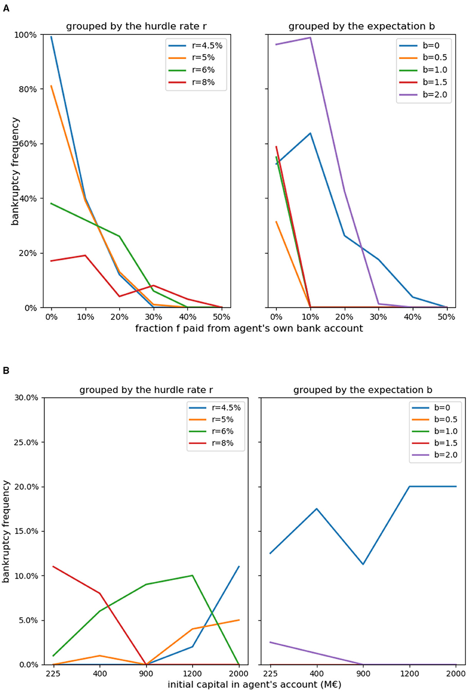
Figure 10. Bankruptcy frequency of agents grouped by hurdle rate r or carbon tax expectation b. (A) Cases with varying f, which is the fraction of an investment financed by a company's own capital; (B) cases with varying i, which is the initial capital in a company's bank account.

Note that when agents have to provide a greater share of the investment from their own capital (higher f), agents are less likely to go bankrupt. Primarily, this is due to a lower debt burden of the companies that reduces the risk for bankruptcy. In addition, when companies are more constrained by capital, there are fewer investments before and during the transient phase and the electricity price is higher compared to when agents are less capital constrained (see Supplementary Figure 3), this leads to a higher return on investments during the transient period. Another reason is that when there is less access to capital, agents also avoid making as many poor investments.

On the other hand, when the required investment payment from agents is very low (i.e., f = 0% or f = 10%), agents are more likely overall to go bankrupt. In these cases, agents are more likely to overinvest, which leads to lower electricity prices than expected, and agents end up not being able to pay back their loans. The reasons why agents overinvest are first that agents have limited foresight of future carbon prices, and some agents expect much higher carbon prices than the actual development. For example, in the case f = 0%, agents with high expectations for the pace of the increase in the carbon price (b=1.5 or 2.0) invest heavily in wind in the beginning (see Figure 14). The second reason is that agents have limited information about other agents' investment decisions. Since agents take turns making investment decisions, agents do not have information about subsequent investments made by other agents. An investment that initially seemed profitable can become unprofitable when subsequent investments are made.

Figure 10 also illustrates that agents with different characteristics (r and b) perform differently in terms of the likelihood of going bankrupt. Some agents are more prone to go bankrupt, while some others do well, financially in most situations.

When comparing agents in terms of hurdle rates, agents using low hurdle rates are more likely to go bankrupt. Because these agents make more investments (than agents with higher hurdle rates), they face more risk as well, as each investment is associated with risk.

Comparing agents in terms of their different expectations on the development of the carbon price, the agents who expect the lowest (b = 0) or highest (b = 2) carbon prices are more likely to go bankrupt. Agents expecting the lowest carbon price make unprofitable investments in coal plants because they underestimate future carbon prices, while agents expecting the highest carbon price go bankrupt as a result of their unsuccessful investments in gas and gasCCS plants during the early years of the transition (see IRR in Figure 3 above). The reason these agents invest in gas plants is that they overestimate carbon prices to the extent that they think that natural gas will be placed ahead of coal in the merit order and hence think that gas plants will become profitable. However, gas will in fact only be ahead of coal in the merit order much later⁴.

Impact of Financial Module

In addition, we test the model without the financial feedback module, which means that an agent will not go bankrupt when its equity goes to zero, and it can get a full loan (100%) from the bank regardless of its financial condition.

Figure 11 shows that overall investment is dominated by a single agent who employs the lowest hurdle rate (r = 4.5%/yr) and the highest carbon tax (b = 2). This agent is more willing to invest than others by virtue of not only requiring a lower return but also perceiving higher future electricity prices by overestimating the carbon tax. Since bankruptcy is not implemented, this agent can make as many investments as it thinks would be profitable. These investments lower the overall electricity price and crowd out other agents who either require a higher return (i.e., apply higher hurdle rates) or expect a lower future carbon tax. Only after the carbon tax starts to stabilize do the four other agents with the lowest hurdle rate (r = 4.5%/yr) begin to invest similarly to the dominant agent, at that point foreseeing the same future carbon prices, see Equation (1).

FIGURE 11

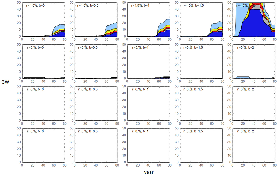
Figure 11. Capacity mix of individual agents when financial feedback module is not implemented, which means an agent does not go bankrupt and can borrow 100% from the bank regardless of its financial situation.

Comparing the case above with the regular case of f = 0%, in which an agent can get a full loan from the bank (agent pays 0% from its own capital) only if its bank account is not negative, and the bankruptcy mechanism is implemented (an agent goes bankrupt if its equity goes to zero), we see that the dominating agent in the previous case goes bankrupt in this case (Figure 12). This discrepancy illustrates that financial mechanisms may strongly affect the agents' performance results, which accentuates that care is needed in the design of agent-based models.

FIGURE 12

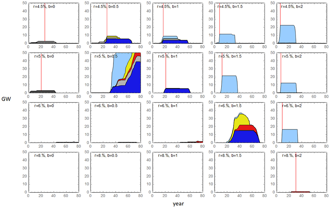
Figure 12. The capacity mix of individual agents when the financial feedback module is implemented and f = 0% and i = 400M€. f is the fraction of an investment financed by a company's own capital, and i is the initial capital in a company's bank account. The vertical red line indicates the year an agent goes bankrupt.

Sensitivity Analysis

To test the robustness of the model results, we investigated the impact of the growth rate of the carbon tax. We test how the increasing rate of the carbon tax impacts agents' investment patterns and the pace of emission reductions. Instead of increasing the tax by 2€ per ton CO₂/year, here we test both a slower and a faster growth rate. In the slow case, the tax starts to increase by 1€ per ton after 10 years, reaching 100€/ton in year 110. In the fast case, the tax rises by 4€ per ton CO₂/year, and reaches 100€/ton in year 35 and stays there. All other parameters are the same as in the base case, see section Set-up of the experiment.

As expected, emissions are cut more rapidly when the tax grows faster but more slowly when the tax grows slower (Figure 13). This is mainly due to agents investing earlier in low-carbon technologies, and also invest more in gas plants with CCS when the tax grows faster (see Supplementary Figure 4).

FIGURE 13

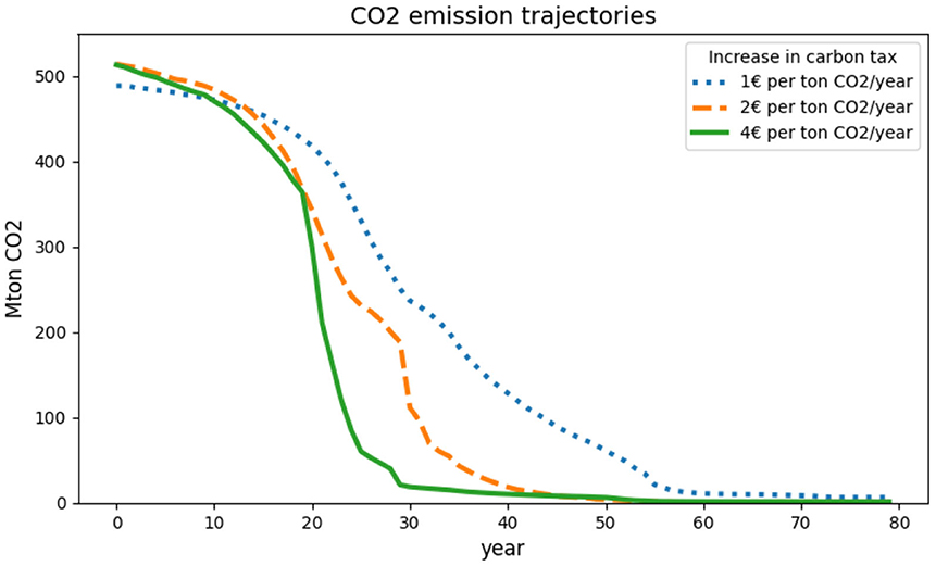
Figure 13. Emission trajectories for three different carbon tax scenarios. In the base case the tax increases by 2€ ton CO₂/year, and the sensitivity analysis tests a faster increase case (4€ ton CO₂/year) and a slower increase case (1€ ton CO₂/year).

Looking at agent's performances, with a faster tax increase, there is overall a greater tendency to go bankrupt (Figure 14), especially for agents expecting the carbon tax to increase rapidly relative to this faster increase (b = 1.5 and b = 2). Meanwhile, when the tax increases slowly at 1€ per ton CO₂/year, no agents go bankrupt.

FIGURE 14

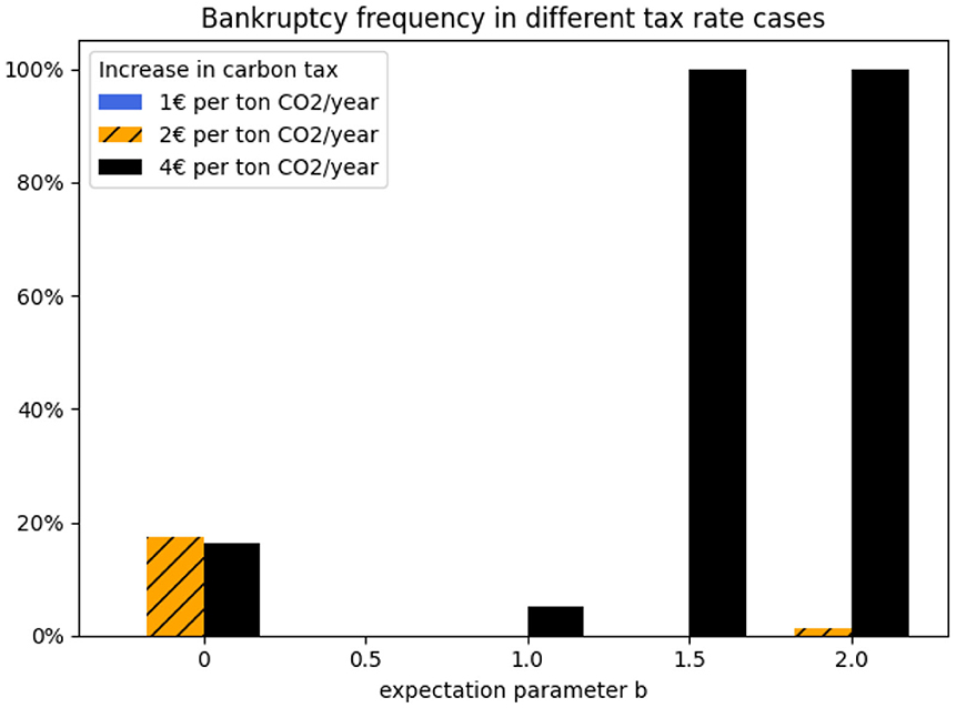
Figure 14. Bankrupt tendency in three different carbon tax scenarios. Note that no agents go bankrupt in the slow tax-increase scenario (increase rate = 1€ per ton CO₂/year), therefore, the bar is not visible in the figure.

The four agents expecting the fastest increase in the carbon tax relative to the actual development (b = 2) go bankrupt in 100% of the 20 runs when the actual tax increase is fast, due to their unprofitable investments in gas and gasCCS plants in the early years (before year 30). In this fast tax-increase case, the IRRs of gas and gasCCS investments (Figure 15) are even lower than in the base case (Figure 3). The higher tax increases the fuel cost of the gas-fired plant. In contrast, the return of wind investment before year 30 is higher than in the base case. This is because the higher tax level leads to higher electricity prices, which benefit wind plants.

FIGURE 15

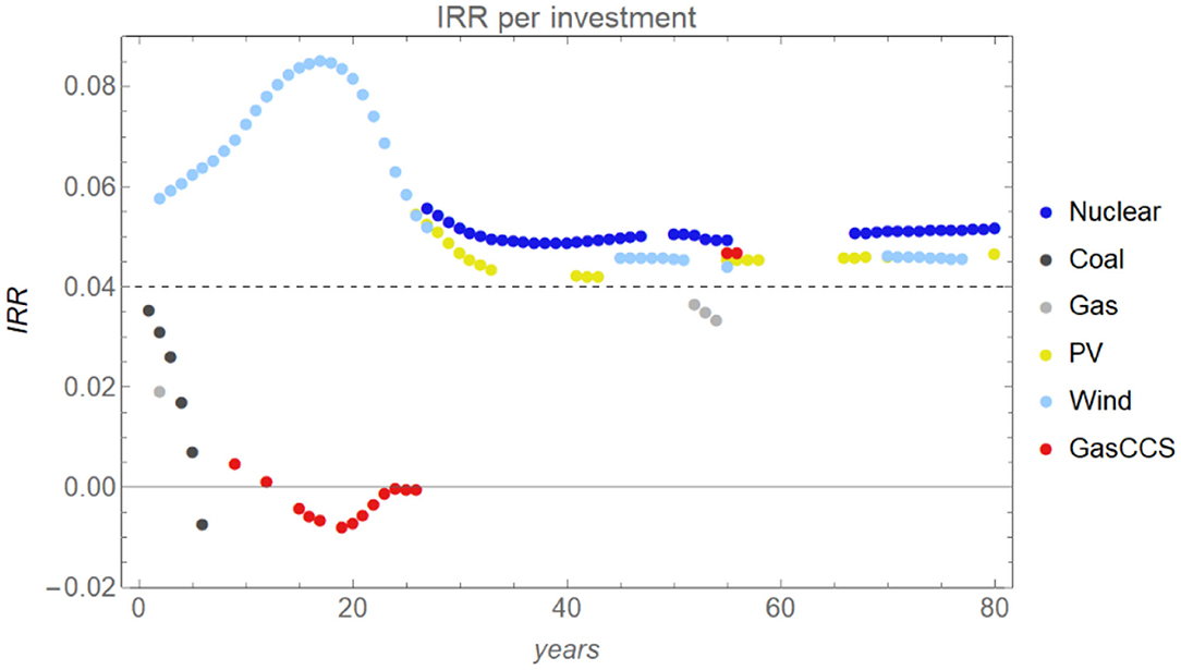
Figure 15. Internal rate of return (IRR) in the fast tax-increase case (increase rate = 4€ per ton CO₂/year). Each dot indicates the IRR of an investment made in a particular year. The horizontal dash line indicates the 4% bank interest rate.

Conclusion

In order to solve the climate challenge, substantial investments in low-carbon technologies are required. This raises the question of how these investments should be financed. In most integrated assessment models, including optimisation-based models of the energy system, access to capital is never a problem since the cost-effective solution by default is (most often) implemented. However, in reality access to capital as well as companies' willingness to take risks by increasing their debt financing—in particular in light of significant uncertainty in future carbon, fuel and electricity prices—may be a critical constraint on the transition to a low carbon society. For that reason, there is a growing interest in the financial sector and the role it may play to facilitate the transition to a low-carbon society.

In this study, we introduce an agent-based model of the electricity system called HAPPI (Heterogenous Agent-based Power Plant Investments model), which includes an explicit module of how investments are financed and that keeps track of companies' debt and equity over time. If the bottom line of a company develops poorly, it will face increasing difficulties in financing new investments.

We examine the financial module's effect on results for the transition to a low-carbon electricity system under an increasing carbon tax scenario. We pay special attention to the impact of financial constraints and electricity demand on the agents' investment decisions and financial performance and, in turn, on the transition of the electricity system.

Our results show that, when agents are more constrained by capital, there are delays in investments in the low-carbon technologies with high investment costs such as wind, solar, and nuclear, and this results in slower emission reductions compared to when capital is more easily accessible. This suggests that rapidly decarbonising the electricity sector could require government incentives that reduce risks for investors.

Our results also show that during the transient period, when the carbon tax is increasing, profits are rather high. This is a non-equilibrium feature in the model: agents have limited ability to make new investments because they have not accumulated a sufficient amount of capital of their own and access to capital is restricted since agents must supply a certain fraction of any new investment from their own bank account (the remaining part of the investment can be borrowed as a loan from the bank). These constraints lead to higher electricity prices and, therefore, higher returns on investment.

Our model also illustrates that, in general, companies that expect too low or too high carbon prices run a greater risk of going bankrupt and their return on equity is in general worse than companies that have a more correct expectation of the future carbon tax. Results also show that a higher tax growth rate leads to a higher risk of bankruptcy, while companies are less likely to go bankrupt under a slow tax-increase scenario. This implies a role for government to help investors by giving clear signals regarding a steady increase in the carbon tax.

Furthermore, our results illustrate the trade-off between lower risk and higher returns. Agents that use low hurdle rates invest more and take a larger market share and tend to enjoy higher returns on equity. Our results also show that agents overall are more prone to going bankrupt when they are more exposed to uncertainties, such as volatile fuel prices and fluctuating electricity demand.

Finally, we want to draw attention to the following three points in the context of agent-based modeling. The first point is whether and how to include a financial module, as well as the assumptions about parameter values for the financial module have significant importance for the investment behavior among the agents. This may not in itself be surprising, but since this feature is most often neglected in energy systems studies, more effort is needed to better model how financing conditions affect energy investments at the individual agent as well as at the overall system level.

Secondly, in optimisation models, the expansion of various energy technologies is typically constrained by setting an arbitrary maximum expansion rate. However, in our model the expansion rate is partly constrained as a result of (limited) access to financial capital. We think that the approach employed here may provide a possible way to explore limits to the expansion rate in an endogenous manner rather than through arbitrary exogenous assumptions. But clearly, there is a long way forward before clear-cut modeling answers can be provided to these complex matters.

Thirdly, our results pertaining to the economic performance of companies who believe the carbon tax will be higher than it really turns out to be are interesting for the broad societal and academic discussion about whether pro-active companies may become more profitable than companies that only respond slowly to environmental regulations. We found as stated above, here that companies that assume that the carbon tax will grow twice as fast as it eventually does perform worse economically than those who have a more correct expectation. Also, companies that do not think that the tax will increase at all perform much worse. Although the answer to the question of how companies may navigate the uncertainty about possible future environmental regulation and changes in consumer demand is complex and the answers provided here are not set in stone, analyzing the energy system transition using agent-based models rather than optimisation models is necessary if one wants to understand the potential impact (economic return) of different companies' investments strategies. In an agent-based model, companies may make both wise and erroneous decisions, whereas in an optimisation model there are typically only one central agent and actors typically have perfect foresight and make only optimal decisions. Hence, in the future, we hope to analyse in more depth the impact of various strategies for different companies.

Data Availability Statement

The model is programmed in Wolfram Mathematica (version 12.1) and Python (version 3.7). The model code, data and documentation are available online at https://github.com/happiABM/HAPPI.

Author Contributions

KL and CA conceived the idea, with contributions from JY. KL, CA, and JY further developed the model, designed model experiments, and analyzed the results. JY wrote the paper with contributions from CA and KL. All authors contributed to the article and approved the submitted version.

Funding

JY receives funding from ENSYSTRA (with funding through the European Union's Horizon 2020 research and innovation programme under the Marie Skłodowska-Curie Grant Agreement No 765515). CA and KL have received funding from the Carl Bennet AB, Mistra electric transition, SWECO/Richert and the Technology Governance program under Chalmers Area of Advance Energy.

Conflict of Interest

The authors declare that the research was conducted in the absence of any commercial or financial relationships that could be construed as a potential conflict of interest.

Publisher's Note

All claims expressed in this article are solely those of the authors and do not necessarily represent those of their affiliated organizations, or those of the publisher, the editors and the reviewers. Any product that may be evaluated in this article, or claim that may be made by its manufacturer, is not guaranteed or endorsed by the publisher.

Acknowledgments

We would also like to thank Paulina Essunger, Markus Wråke, Göran Carstedt, Stefan Park, Cookie Belfrage, Daniel Johansson, and Linda Burenius for valuable discussions and suggestions.

Supplementary Material

The Supplementary Material for this article can be found online at: https://www.frontiersin.org/articles/10.3389/fclim.2021.738286/full#supplementary-material

Footnotes

1. ^Were decisions to be made with parameters kept as in the base case, this would correspond to a stationary zero carbon tax situation.

2. ^The reason we use 225 M€ instead of 200 M€ is that, with 200 M€ initial capital (and f = 30%), a company can only start by investing in a gas-fired plant. We want to avoid this model artifact. With initial capital of 225 M€ (and f = 30%), a company can afford to invest in any kind of plant except nuclear.

3. ^Note that the agent with r = 4.5%/yr and b = 0 invested only in coal power plants in the beginning but did not go bankrupt. The coal power plants receive annual net revenues that covers the costs of loans (i.e., positive annual net profit) for the first 20–25 years, but gradually the net profit of coal plants becomes negative resulting in an IRR below the bank interest rate already around year 10. The annual net profit during the later years of the coal power plants life time is compensated for by both the accumulated profit up to around year 20 and the later profitable investments in wind and nuclear. All this makes it possible for the company to survive the bad investments in coal after year 10, keeping a positive equity level avoiding bankruptcy.

4. ^We have also tested in a setting where gasCCS is not available, and then agents with b = 2 perform poorly too and sometimes go bankrupt, so the result is more general than the individual pathway described here.

References

Azar, C., Johansson, D., and Mattsson, N. (2013). Meeting global temperature targets-the role of bioenergy with carbon capture and storage. Environ. Res. Lett. 8:034004. doi: 10.1088/1748-9326/8/3/034004

CrossRef Full Text | Google Scholar

Azar, C., Lindgren, K., and Andersson, B. A. (2003). Global energy scenarios meeting stringent CO2 constraints—cost-effective fuel choices in the transportation sector. Energy Policy 31, 961–976. doi: 10.1016/S0301-4215(02)00139-8

CrossRef Full Text | Google Scholar

Barazza, E., and Strachan, N. (2020). The impact of heterogeneous market players with bounded-rationality on the electricity sector low-carbon transition. Energy Policy 138:111274. doi: 10.1016/j.enpol.2020.111274

CrossRef Full Text | Google Scholar

Battiston, S., Monasterolo, I., Riahi, K., and van Ruijven, B. J. (2021). Accounting for finance is key for climate mitigation pathways. Science 372, 918–920. doi: 10.1126/science.abf3877

PubMed Abstract | CrossRef Full Text | Google Scholar

Chappin, E. J. L., de Vries, L. J., Richstein, J. C., Bhagwat, P., Iychettira, K., and Khan, S. (2017). Simulating climate and energy policy with agent-based modelling: the energy modelling laboratory (EMLab). Environ. Model. Softw. 96, 421–431. doi: 10.1016/j.envsoft.2017.07.009

CrossRef Full Text | Google Scholar

DiaCore (2016). The Impact of Risks in Renewable Energy Investments and the Role of Smart Policies. Brussels: European Commission.

Google Scholar

Econometrics, C. (2019). E3ME Technical Manual v6.1. Cambridge: Cambridge Econometrics.

Google Scholar

EIA (2019). The National Energy Modeling System: An Overview 2018. Washington, DC: U.S. Energy Information Administration.

EIA (2020). The Electricity Market Module of the National Energy Modeling System: Model Documentation 2020. Washington, DC: U.S. Energy Information Administration.

FS-UNEP BNEF. (2019). Global Trends in Renewable Energy Investment 2019. Frankfurt: Frankfurt School-UNEP and BloombergNEF.

FS-UNEP BNEF. (2020). Global Trends in Renewable Energy Investment 2020. Frankfurt am Main: Frankfurt School of Finance and Management.

Google Scholar

Genoese, M. (2010). Energiewirtschaftliche Analysen Des Deutschen Strommarkts Mit Agentenbasierter Simulation, 1st edn. Baden-Baden: Nomos Verlagsgesellschaft mbH & Co. KG. doi: 10.5771/9783845227443

PubMed Abstract | CrossRef Full Text | Google Scholar

Gerst, M. D., Wang, P., Roventini, A., Fagiolo, G., Dosi, G., Howarth, R. B., et al. (2013). Agent-based modeling of climate policy: an introduction to the ENGAGE multi-level model framework. Environ. Model. Softw. 44, 62–75. doi: 10.1016/j.envsoft.2012.09.002

CrossRef Full Text | Google Scholar

IEA (2019). World Energy Investment 2019. Paris: International Energy Agency.

IEA (2020). CO2 Emissions From Fuel Combustion. Paris: International Energy Agency.

IRENA (2018). Renewable Power Generation Costs in 2017. Abu Dhabi: International Renewable Energy Agency.

IRENA (2020a). Global Renewables Outlook: Energy transformation 2050. Abu Dhabi: International Renewable Energy Agency.

IRENA (2020b). Renewable Energy Finance: Institutional Capital. Abu Dhabi: International Renewable Energy Agency.

Jonson, E., Azar, C., Lindgren, K., and Lundberg, L. (2020). Exploring the competition between variable renewable electricity and a carbon-neutral baseload technology. Energy Syst. 11, 21–44. doi: 10.1007/s12667-018-0308-6

CrossRef Full Text | Google Scholar

Kraan, O., Kramer, G. J., and Nikolic, I. (2018). Investment in the future electricity system - an agent-based modelling approach. Energy 151, 569–580. doi: 10.1016/j.energy.2018.03.092

CrossRef Full Text | Google Scholar

Loulou, R., Remne, U., Kanudia, A., Lehtila, A., and Goldstein, G. (2005). Documentation for the TIMES Model. Paris: International Energy Agency.

Myers, S. C., and Majluf, N. S. (1984). Corporate financing and investment decisions when firms have information that investors do not have. J. Financial Econ. 13, 187–221.

Google Scholar

NTUA EMI. (2014). PRIMES MODEL 2013-2014 Detailed Model Description. Athens: NTUA and EMI.

Pollitt, H., and Mercure, J.-F. (2018). The role of money and the financial sector in energy-economy models used for assessing climate and energy policy. Clim. Policy 18, 184–197. doi: 10.1080/14693062.2016.1277685

CrossRef Full Text | Google Scholar

Ponta, L., Raberto, M., Teglio, A., and Cincotti, S. (2018). An agent-based stock-flow consistent model of the sustainable transition in the energy sector. Ecol. Econ. 145, 274–300. doi: 10.1016/j.ecolecon.2017.08.022

CrossRef Full Text | Google Scholar

Safarzynska, K., and van den Bergh, J. C. J. M. (2017). Financial stability at risk due to investing rapidly in renewable energy. Energy Policy 108, 12–20. doi: 10.1016/j.enpol.2017.05.042

CrossRef Full Text | Google Scholar

Sepulveda, N. A., Jenkins, J. D., de Sisternes, F. J., and Lester, R. K. (2018). The role of firm low-carbon electricity resources in deep decarbonization of power generation. Joule 2, 2403–2420. doi: 10.1016/j.joule.2018.08.006

CrossRef Full Text | Google Scholar

Yang, J. (2021). Transition to a Low-carbon Electricity System - Investment Decisions Under Heterogeneity, Uncertainty and Financial Feedback [Licentiate thesis]. Department of Space, Earth and Environment. Chalmers University of Technology. Available online at: https://research.chalmers.se/en/publication/525564

Google Scholar