Reading Single Words Aloud With Monocular Presentation: The Effect of Word Frequency

Introduction

A robust finding in reading research is that common words are read faster and more accurately than less common ones. A word frequency effect is observed in single word reading aloud, lexical decision, sentence reading, same-different matching, and using many measures: reaction time, errors, gaze duration, fixation times, detection thresholds and so on (e.g., see Howes and Solomon, 1951; Broadbent, 1967; Morton, 1968; Rayner and Duffy, 1986; among many others). A notable exception are the results seen in Jainta et al. (2014, 2017). They report, in two eye-tracking studies, that the word frequency effect is eliminated (or reduced) when participants read sentences with only one eye (monocular reading). Such results are potentially problematic for all current theoretical accounts of reading at the single word level; the Jainta and colleagues results thus merit close attention in the context of such accounts.

Jainta et al. (2014) used a gaze contingent viewing paradigm, manipulating whether the target word in a sentence was viewed with only one or both eyes. They found that when English sentences were read with one eye, the processing benefit for high frequency words was eliminated in both gaze duration and fixation times (Jainta et al., 2014, jointly manipulated the preview reading conditions and the target reading conditions—preview benefits are not relevant to our study, so we focus only on the viewing conditions when reading the target words). Jainta et al. (2017) observed the same elimination of the frequency effect under monocular reading conditions for gaze duration and first fixation times in German. The total reading time measure continued to show a word frequency effect (one-tailed) under monocular conditions, but it was less than half the magnitude of the effect under binocular conditions (see Figure 1). To account for the absence/reduction of word frequency effects under monocular reading conditions the authors appeal to the level of neural activity in visual cortex during binocular reading. They suggest that increased neural activity during binocular reading feeds into the lexical system and provides an advantage, particularly to high frequency items (and exclusively to high frequency words in their data). This advantage is lost during monocular reading, hence eliminating the word frequency effect.

FIGURE 1

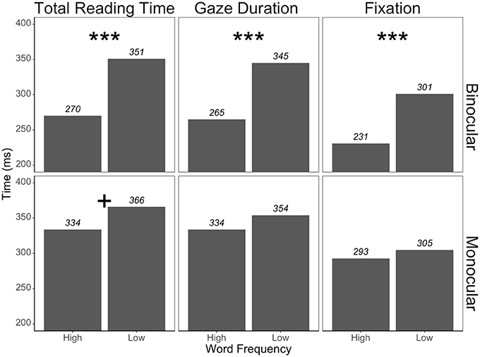
Figure 1. Results from Jainta et al. (2017) Experiment 1. ***p < 0.01, ⁺p < 0.10.

The neural activity account may be intrinsically specific to sentences or eye-tracking (indeed, the authors have couched their account in such terms) but it seems obvious (at least to us) that word recognition researchers would want to know whether this elimination (or reduction) of the word frequency effect is also seen in single word reading.

Although current models of single word reading (reading aloud for example) have not, as yet, considered manipulations such as monocular/binocular reading, they would be hard-pressed to account for the absence (or reduction) of a word frequency effect under any conditions. To be sure, localist computational models such as DRC (Coltheart et al., 2001) and CDP++ (Perry et al., 2010) may be able to simulate this absence of a word frequency effect under a monocular condition by assuming that binocular vision influences the frequency tuning parameter (though we doubt those authors would find that account appealing). Even with that possibility in mind, however, the Jainta et al. results challenge, at the very least, the way the effect of word frequency is implemented in these models. Both DRC and CDP++ use the tuning parameter to depress activation as a function of frequency. Reducing the tuning parameter would thus speed the low frequency items rather than slowing the high frequency items, as observed by Jainta et al. (in fact, it would speed all items).

Relatedly, computational models based on PDP principles (Plaut et al., 1996 and its descendants), implement frequency as the natural result of repeated exposures and the consequent changing of connection weights. Consequently, these models could not possibly explain both the presence of a word frequency effect during binocular reading, but its absence during monocular reading. The back-propagation algorithm used in such models simply cannot avoid a frequency effect. Indeed, we are unable to conceive how such models could even show a reduction of the word frequency effect due only to slowing of high frequency items. In short, the results reported by Jainta et al. (2014, 2017) should they generalize to single word reading experiments, would strongly challenge current thinking about one of the most widely accepted benchmarks used to evaluate accounts of single word reading aloud.

We wish to stress that we are not challenging Jainta and colleagues' results. Rather, we ask a simple question: will a standard word recognition paradigm (the reading aloud of single words) produce the same pattern of data as seen in the eye tracking data reported by Jainta and colleagues. This is in the spirit of Schilling et al. (1998, p. 1277) who compared lexical decision, reading aloud, and eye movement measures, and reported significant correlations across these three measures. They concluded that “both the naming and lexical decision tasks yield data concerning word recognition processes that are consistent with effects found in silent reading.”

Hence, if we observe the same pattern in reading aloud as seen in the eye tracking studies reported by Jainta and colleagues (a reduction in the size of the word frequency effect under monocular as compared to binocular conditions) this would present a fundamental challenge to all accounts of visual word recognition currently on the table. On the other hand, if we do not see the same pattern in single word reading aloud as in the eye movement studies, then this is consistent with the hypothesis this dissociation is deeply intertwined with the control of eye movements, as Jainta and colleagues suggested.

The Experiment

The design of the experiment is simple. Participants read words aloud under both monocular (one eye covered with an eyepatch) and binocular reading conditions. We note that this study design was informally pre-registered at https://osf.io/fxcjv/. Stimuli, data and analysis scripts are available at (https://osf.io/t9dux/), and deviations from the preregistration are clearly identified in the text.

Method

Participants

Participants were sampled from the pool of undergraduate psychology students at the University of Waterloo. They received course credit in exchange for their participation. All participants reported learning English before age 5 (rather than as their first language, as originally planned), and normal or corrected-to-normal vision. In all, 22 participants were recruited. As we planned to use Bayesian analysis techniques, we collected data until the result was clear. Bayesian analysis techniques do not require settling on a sample size before data collection (Rouder, 2014). Our planned stopping rule was as follows: with six counterbalances, we planned to collect 18 subjects before the first analysis, and then to reanalyze the data after every sixth subject. We planned to stop once the Bayes factor for the word frequency effect in the monocular condition clearly favored a conclusion (at least 10x as much evidence in one direction or the other). Due to how the participants arrived in the lab, we had collected 22 subjects by the time the first analysis point occurred, at which point the stopping criteria were met and data collection was terminated. We also note that rather than using the word frequency effect in the monocular condition as our stopping rule, we used the presence or absence of the word frequency by reading condition interaction since this would clearly support the Jainta et al. (2017) account even without a complete elimination of the word frequency effect. In the end, both stopping rules were achieved at the same point so there would have been no difference had we remained with the pre-registered rule.

Design

The experiment had a 2 × 3 within-participants factorial design with word frequency (high vs. low) and reading condition (binocular, left eye, right eye) as factors. Reading condition was blocked with the order of the blocks counterbalanced across participants. Within each block, word frequency was randomized across trials while ensuring an equal number (33) of high and low frequency items in each block, and ensuring that each item appeared in all three reading conditions for approximately equal numbers of participants.

Stimuli

The stimulus list consisted of the words from O'Malley and Besner (2008; Experiment 3). As they had 100 high and low frequency items (and we needed only 99), we randomly removed one high frequency and one low frequency word, so that our 3 lists could be of equal length. Based on the Kucera and Francis (1967) norms, high frequency words ranged from 136 to 4,369 occurrences per million, while low frequency items ranged from 1 to 67 occurrences per million.

Procedure

Participants sat at a comfortable distance from a computer monitor and read words aloud into a microphone. DMDX (Forster and Forster, 2003) controlled the presentation conditions, and recorded reaction times (onset of utterance) and the actual word spoken. Participants read 99 high frequency words and 99 low frequency words, split into three blocks of 33 each. Each block of 66 items was read under one of the reading conditions: binocular reading, monocular reading (left eye), or monocular reading (right eye). Preceding each block, the experiment screens instructed participants to either cover their left or right eye (as appropriate) with a sterilized eye patch provided by the experimenter, or to leave the eye patch on the desk in front of them and read with both eyes. The order of the reading conditions was counter-balanced across participants resulting in six counterbalance conditions. Within a block, items were randomized, though the same 66 items appeared in block 1 (and 2, and 3) for every participant. This avoided the need for 36 counterbalances, while still ensuring that all items appeared equally often in the three reading conditions.

Response accuracy and reaction times were verified by the experimenter using the CheckVocal program (Protopapas, 2007). This allows experimenters to directly examine the recorded waveforms and ensure that the measured reaction times correspond to the onset of the utterance.

Analysis Plan

Statistical methods

As the Jainta et al. (2014) explanation of their data is based on a null effect of word frequency in some conditions, we analyzed the data using trial level mixed effects models and Bayesian Analysis techniques. Bayesian analysis techniques compare the likelihood of one model (a model with no interaction between word frequency and reading condition) to the likelihood of an alternative model (a model with the interaction present). By taking the ratio of the two likelihoods, the Bayes factor indexes the degree to which the evidence (data) favors one hypothesis over the other. By convention, the notation BF₀₁ is used to index the degree to which the evidence favors the null model over an alternative model, while BF₁₀ is the inverse (indeed, the inverse is both theoretical and mathematical: BF₁₀ = 1/BF₀₁).

Data preparation

Two of the participants were removed from analysis – one because they were unable to provide clear responses on most trials, the other due to an extremely high error rate (16% compared to no worse than 7% for any other participant) on Binocular trials. We first removed any microphone misfires, or failures to respond (0.3% of trials), and response errors (3.1% of trials). Jainta et al. (2014, 2017) log-transformed their fixation time measures. To ensure comparability of the DVs, we do the same to our reaction time measure. We then subjected the log reaction times to the Van Selst and Jolicoeur (1994) recursive outlier procedure (removing a further 0.4%). The remaining log reaction times were carried through to the analysis. Though we tested both the left and right eyes, there was no difference between the two and so the reading condition variable was recoded as Binocular vs. Monocular by collapsing the two monocular vision conditions into one.

Analysis procedure

For the analysis, we fit two mixed effects models with identical random structures (maximal for the additive model) and compared them using the BayesFactor package in R (Morey and Rouder, 2015). The additive model was as follows:

$\begin{array}{l}{Y}_{p,i}={\beta }_0+S_{0,p}+I_{0,i}+({\beta }_1+S_{1,p})W{F}_i\\ +({\beta }_2+S_{2,p}+I_{2,i})Vision+e_{p,i}& (1)\end{array}$

where Y_p,i is the natural log of the RT for participant p to item i; S_0,p and I_0,i are random intercepts by participants and items respectively; S_1,p and S_2,p are random slopes for WF and Vision by participant; and I_2,i is the random slope for Vision by item.

This additive model was compared to an interaction model:

$\begin{array}{l}{Y}_{p,i}={\beta }_0+S_{0,p}+I_{0,i}+({\beta }_1+S_{1,p})W{F}_i\\ +({\beta }_2+S_{2,p}+I_{2,i})Vision+{\beta }_{3}WF·Vision+e_{p,i}& (2)\end{array}$

which adds the interaction term (but no random slopes for the interaction). The critical question is whether the interaction model provides a better fit to the data than the null model. Such a result would produce a Bayes factor (BF₀₁) less than 1. A BF₀₁ greater than 1 would favor the absence of such an interaction.

We also planned to compare the word frequency effect for each of the reading conditions to confirm that any interaction was consistent with the pattern expected from Jainta et al. (2014, 2017). To preview the results somewhat, there was little evidence for such an interaction and so this additional analysis was not carried out.

Results

The model predicted means are summarized (along with percentage errors) in Table 1. The experiment provided strong evidence for the null model (no interaction) over the interactive alternative model (BF₀₁ = 12.6 ± 2.36%). That is, the evidence strongly favored the view that the word frequency effect was equivalent in both the monocular and binocular reading conditions. In fact, from Table 1 it is apparent that if there were an interaction, it would go in the wrong direction—monocular reading produced a slightly larger word frequency effect. The implication is that the evidence for the form of the interaction reported by Jainta and colleagues is specific to their eye movement paradigm rather than general to other measures (such as reading aloud, as here). When the Bayes factor is corrected for this directional prediction, the evidence favoring the null model over the Jainta et al. account increases from 12.6 to 23.0 times¹.

TABLE 1

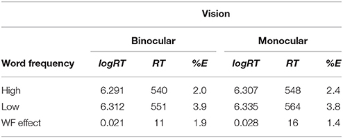
Table 1. Mean log RT, associated RT (ms), and % errors (%E) for the experiment.

Discussion

In contrast to the Jainta et al. (2014, 2017), results with sentence reading, single word reading produces no difference between binocular and monocular reading in the magnitude of the word frequency effect. The present result may thus represents a challenge to their account of the absence of a word frequency effect during monocular reading in sentence reading. If binocular reading per se confers a neural advantage to high frequency items, this experiment should have found an interaction of the same form as observed in the sentence reading experiments. To be sure, Jainta and colleagues never claimed that the pattern they reported would be seen in paradigms other than eye tracking. If the pattern they observed is indeed specific to their eye tracking paradigm then it stands as a clear (no pun intended) example of a dissociation in the processes underlying sentence reading vs. single word reading aloud, and hence the notion (as promulgated by Schilling et al., 1998) that there are common processes across eye movements, reading aloud and lexical decision should be contextualized and qualified.

Additional Analyses

We have not examined the word frequency effect directly here (nor had we planned to in our pre-registration). In this case, however, the analyses reported so far leaves open the possibility that there is no interaction because there is no word frequency effect to begin with. As previously discussed, word frequency effects are virtually always observed in reading aloud studies and the stimuli used here produced a robust word frequency effect in the O'Malley and Besner (2008) study of reading aloud. Consequently, there is little reason to think there would not be a word frequency effect here. Nonetheless, to ensure that the apparent effect of word frequency in Table 1 is genuine, we first looked at the Bayes factor comparing a model with no word frequency effect:

$\begin{array}{ll}{Y}_{p,i}={\beta }_0+S_{0,p}+I_{0,i}+({\beta }_2+S_{2,p}+I_{2,i})Vision+e_{p,i}& (3)\end{array}$

to the original additive model (1). The Bayes factor provided very strong evidence for the presence of a word frequency effect (BF₀₁ = 0.0397 ± 3.17%; BF₁₀ = 25.2).

We also examined the posterior distribution from the additive model (1). To do this we sampled 10,000 values from the posterior distribution. The density of the posterior distribution and the 95% highest density interval (HDI) are plotted in Figure 2. The 95% HDI was obtained from the HDInterval package (Meredith and Kruschke, 2016) and can be thought of as a Bayesian analog to a 95% confidence interval (CI), though it has a slightly different interpretation (a CI does not have any distributional characteristics—there is no sense in which one value within the CI has more or less likelihood of being the true value than any other—meaning that CIs containing zero imply “failure to reject the null”; in contrast, an HDI is distributional in that values near the center of the HDI are more probable than values at the extremes—in this case, much more probable).

FIGURE 2

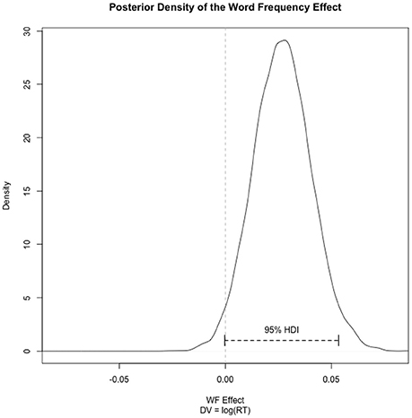
Figure 2. Posterior distribution of the word frequency effect with 95% highest density interval (HDI). Note that there is some density beyond the bounds of the x-axis, but the plot is truncated for clarity.

General Discussion

Jainta et al. (2014, 2017) reported that when reading sentences with only one eye, participants no longer produced the typical word frequency effect in gaze duration or fixation times as seen when compared to a binocular condition. Their account of this result appeals to the idea that there are neural consequences for binocular vs. monocular reading: since there is more neural activity during binocular reading, they reasoned that this must be assisting high frequency words. During monocular reading, this benefit is lost, eliminating the word frequency effect.

These results have implications outside of the sentence reading domain in which the Jainta et al. experiments were conducted. If binocular reading per se confers an advantage to high frequency words because of the increased neural activity in visual cortex, then the same pattern should be evident in the single word reading aloud task. Such an outcome would clearly challenge all current models of single word reading aloud. We therefore asked participants to read aloud high and low frequency words under binocular and monocular reading conditions. In contrast to the findings reported by Jainta and colleagues in two studies, we observed no interaction between word frequency and monocular/binocular reading. Indeed, our data provided 46.0 times as much evidence against a smaller monocular word frequency effect.

Unresolved Issues

One difference between the present experiment and those by Jainta et al. (2014, 2017) is in the method of controlling vision. In the eye tracking experiments, a pair of goggles permitted the researchers to intermix monocular and binocular reading trials. Here we used a much simpler eye patch, which required us to block the reading conditions. There are situations in which blocking would be inappropriate—for example in an experiment using a contrast manipulation (dim stimuli on a dark background vs. bright stimuli on the same background), we would not at all be surprised if blocking the low- and high-contrast conditions eliminated the contrast effect that is typically seen when trials are intermixed. In this case, the eye is well-designed to adapt to the low-light circumstance and could compensate for the change during blocks of low-contrast displays.

One might raise a similar concern here, but would have to do so with caution. The increased activity in the visual cortex during binocular vision is presumably due to the information arriving from both eyes rather than a single eye. This fact does not change whether the trials are blocked or intermixed. It seems unlikely to us that the visual cortex would adapt to monocular vision in the same way that the eyes do to low light.

Conclusion

It is possible, as Jainta and colleagues seem to imply, that there is a fundamental difference between sentence reading and single word reading in the way that monocular reading functions. Again, the present study does not, in any way, undermine Jainta and colleagues observations. Indeed, there are other reasons to believe that not all manipulations are equivalent across the two contexts. For example, it is well established in the single word reading aloud literature that when both word frequency and stimulus quality are manipulated, these two factors interact in such a way that the stimulus quality effect is larger for low frequency words than for high (at least when reading only words; see O'Malley and Besner, 2008). In contrast, Jainta et al. (2017) manipulated these two factors in a sentence reading task in two experiments and found that they had additive effects (there was no difference in the magnitude of the stimulus quality effect across word frequency). This result, to us, is another interesting example of a dissociation between factors across eye movement paradigms and single word reading aloud, and one that merits further theoretical attention. We (again) stress that we have no basis for thinking that Jainta and colleagues results are not a genuine phenomenon (they did, after all, report the same effect in two experiments, one in English and one in German). The general challenge, we submit, rests in framing their results (and ours) in a broader theoretical context so as to provide a more nuanced and context dependent view of how visual word identification unfolds over time.

Ethics Statement

This study was carried out in compliance with the University of Waterloo Statement on Human Research and with the approval of the Office for Research Ethics at the University of Waterloo, Canada (OHRAC@uwaterloo.ca) with written informed consent from all subjects.

Author Contributions

This manuscript represents the joint efforts of the two authors. Facilities provided by University of Waterloo, Canada. Analyses conducted by senior author. Manuscript written jointly.

Funding

Funding for this project was provided by the Natural Sciences and Engineering Research Council of Canada [A0998] to DB and was approved by the Office of Research Ethics at the University of Waterloo. This includes informed written consent by participants in accord with the Declaration of Helsinki.

Conflict of Interest Statement

The authors declare that the research was conducted in the absence of any commercial or financial relationships that could be construed as a potential conflict of interest.

Footnotes

1. ^The BayesFactor package in R does not allow directly specifying a one-tailed prior. To correct for the direction of the predicted effects, we followed Richard Morey's advice here: http://bayesfactor.blogspot.com/2015/01/multiple-comparisons-with-bayesfactor-2.html and adjusted the BF₁₀ for the proportion of the posterior distribution that was consistent with the Jainta et al. data. See the scripts and data for details.

References

Broadbent, D. E. (1967). Word-frequency effect and response bias. Psychol. Rev. 74, l−15. doi: 10.1037/h0024206

PubMed Abstract | CrossRef Full Text | Google Scholar

Coltheart, M., Rastle, K., Perry, C., Langdon, R., and Ziegler, J. C. (2001). DRC: A dual route cascaded model of visual word recognition and reading aloud. Psychol. Rev. 108, 204–256. doi: 10.1037/0033-295X.108.1.204

PubMed Abstract | CrossRef Full Text | Google Scholar

Forster, K. I., and Forster, J. C. (2003). DMDX: a windows display program with millisecond accuracy. Behav. Res. Methods Instrum. Comput. 35, 116–124. doi: 10.3758/BF03195503

PubMed Abstract | CrossRef Full Text | Google Scholar

Howes, D. H., and Solomon, R. L. (1951). Visual duration threshold as a function of word probability. J. Exp. Psychol. 41, 401–410. doi: 10.1037/h0056020

PubMed Abstract | CrossRef Full Text | Google Scholar

Jainta, S., Blythe, H. I., and Liversedge, S. (2014). Binocular advantages in reading. Curr. Biol. 24, 526–530. doi: 10.1016/j.cub.2014.01.014

PubMed Abstract | CrossRef Full Text | Google Scholar

Jainta, S., Nikolova, M., and Liversedge, S. (2017). Does text contrast mediate binocular advantages in reading? J. Exp. Psychol. Hum. Percept. Perform. 43, 55–68. doi: 10.1037/xhp0000293

PubMed Abstract | CrossRef Full Text | Google Scholar

Kucera, H., and Francis, W. N. (1967). Computational Analysis of Present-Day American English. Providence: Brown University Press.

Meredith, M., and Kruschke, J. (2016). HDInterval: Highest (Posterior) Density Intervals. R package version 0.1.3. Available online at: https://CRAN.R-project.org/package=HDInterval

Morey, R. D., and Rouder, J. N. (2015). BayesFactor: Computation of Bayes Factors for Common Designs. R package version 0.9.12-2. Available online at: https://CRAN.R-project.org/package=BayesFactor

Morton, J. (1968). A retest of the response-bias explanation of the word frequency effect. Br. J. Math. Stat. Psychol. 21, 21–33. doi: 10.1111/j.2044-8317.1968.tb00396.x

CrossRef Full Text | Google Scholar

O'Malley, S., and Besner, D. (2008). Reading aloud: qualitative differences in the relation between stimulus quality and word frequency as a function of context. J. Exp. Psychol. Learn. Mem. Cogn. 34, 1400–1411. doi: 10.1037/a0013084.

PubMed Abstract | CrossRef Full Text | Google Scholar

Perry, C., Ziegler, J. C., and Zorzi, M. (2010). Beyond single syllables: Large-scale modeling of reading aloud with the Connectionist Dual Process (CDP++) model. Cogn. Psychol. 61, 106–151. doi: 10.1016/j.cogpsych.2010.04.001

PubMed Abstract | CrossRef Full Text | Google Scholar

Plaut, D. C., McClelland, J. L., Seidenberg, M. S., and Patterson, K. (1996). Understanding normal and impaired word reading: computational principles in quasi-regular domains. Psychol. Rev. 103, 56–115. doi: 10.1037/0033-295X.103.1.56

PubMed Abstract | CrossRef Full Text | Google Scholar

Protopapas, A. (2007). CheckVocal: a program to facilitate checking the accuracy and response time of vocal responses from DMDX. Behav. Res. Methods 39, 859–862. doi: 10.3758/BF03192979

PubMed Abstract | CrossRef Full Text | Google Scholar

Rayner, K., and Duffy, S. A. (1986). Lexical complexity and fixation times in reading: effects of word frequency, verb complexity, and lexical ambiguity. Mem. Cognit. 14, 191–201.

PubMed Abstract | Google Scholar

Rouder, J. (2014). Optional stopping: no problem for Bayesians. Psychon. Bull. Rev. 21, 301–308. doi: 10.3758/s13423-014-0595-4

PubMed Abstract | CrossRef Full Text | Google Scholar

Schilling, H. H., Rayner, K., and Chumbley, J. I. (1998). Comparing naming, lexical decision, and eye fixation times: word frequency effects and individual differences. Mem. Cognit. 26, 1270–1281. doi: 10.3758/BF03201199

PubMed Abstract | CrossRef Full Text | Google Scholar

Van Selst, M., and Jolicoeur, P. (1994). A solution to the effect of sample size on outlier estimation. Q. J. Exp. Psychol. 47, 631–650. doi: 10.1080/14640749408401131

CrossRef Full Text | Google Scholar