Left-deep join order selection with higher-order unconstrained binary optimization on quantum computers

Join order optimization is among the most crucial query optimization problems, and its central position is also evident in the new research field where quantum computing is applied to database optimization and data management. In this field, join order optimization is the most studied database problem, typically tackled with a quadratic unconstrained binary optimization model, which is solved using various meta-heuristics, such as quantum and digital annealing, the quantum approximate optimization algorithm, or the variational quantum eigensolver. In this study, we continue developing quantum computing techniques for left-deep join order optimization by presenting three novel quantum optimization algorithms. These algorithms are based on a higher-order unconstrained binary optimization model, which is a generalization of the quadratic model and has not previously been applied to database problems. Theoretically, these optimization problems naturally map to universal quantum computers and quantum annealers. Compared to previous studies, two of our algorithms are the first quantum algorithms to model the join order cost function precisely. We prove theoretical bounds by showing that these two methods encode the same plans as the dynamic programming algorithm with respect to the query graph, which provides the optimal result up to cross products. The third algorithm achieves plans at least as good as those of the greedy algorithm with respect to the query graph. These results establish a meaningful theoretical connection between classical and quantum algorithms for selecting left-deep join orders. To demonstrate the practical usability of our algorithms, we have conducted an extensive experimental evaluation on thousands of clique, cycle, star, tree, and chain query graphs using both quantum and classical solvers.

1 Introduction

Join order optimization is one of the critical stages in query optimization, where the goal is to determine the most efficient sequence in which joins should be performed (Selinger et al., 1979). Join order optimization plays a central role, as the order of joins determines whether a query finishes in seconds or hours, especially in large databases (Neumann and Radke, 2018). The problem is a well-researched NP-hard problem (Ibaraki and Kameda, 1984) with various exhaustive and heuristic solutions (Leis et al., 2015; Steinbrunn et al., 1997). The central position of join order optimization in database research is also evident in the new research field where quantum computing is applied to database optimization and data management (Schönberger, 2022; Uotila, 2022). In this subfield, the join order selection problem is the most studied (Schönberger et al., 2023a; Winker et al., 2023a; Schönberger et al., 2023c; Nayak et al., 2024; Franz et al., 2024; Schönberger et al., 2023b; Saxena et al., 2024; Liu et al., 2025; Çalikyilmaz et al., 2023). In contrast, other quantum computing problems related to database and data management include index selection (Gruenwald et al., 2023; Trummer and Venturelli, 2024), cardinality and query metric estimations (Uotila, 2024a, 2025b; Kittelmann et al., 2024), transaction scheduling (Bittner and Groppe, 2020; Nayak et al., 2025), resource allocation (Uotila and Lu, 2023; Trummer, 2025), schema matching (Fritsch and Scherzinger, 2023), relational deep learning (Vogrin et al., 2024), and multiple query optimization (Trummer and Koch, 2016).

Despite the interest in optimizing databases with quantum computers, demonstrating a clear quantum advantage in database-related problems remains open. Generally, demonstrating an advantage of quantum over classical algorithms has proved challenging in practice. Some experiments demonstrate specific forms of quantum advantage (Arute et al., 2019; Harrow and Montanaro, 2017; Kim et al., 2023; King et al., 2024; Madsen et al., 2022; Zhong et al., 2020; Zhu et al., 2021), but none show widely accepted benefits over classical algorithms in real-life applications. On the other hand, some algorithms such as Shor's (1994) and Grover's (1996) algorithms show a provable advantage over the best classical algorithms on fault-tolerant quantum computers, which do not yet exist.

Since demonstrating benefits from current quantum computers has proved challenging, Schönberger et al. (2023b) suggested moving from quantum hardware to quantum-inspired hardware, especially in join order optimization. They argued that special-purpose solvers and hardware, such as digital annealers, should be used. While they demonstrated that this direction is promising and feasible, they did not extensively examine the potential benefits of modifying the underlying quantum optimization model, which has been similar to the previous mixed-integer linear programming solution for the join order selection problem (Trummer and Koch, 2017).

If we seek (database) applications that are likely to benefit from quantum computing, one of our central arguments is that we might want to move from quadratic to higher-order models. Focusing on the quantum computing paradigm that is restricted to quadratic interactions between qubits, previous studies has shown that there are only particular problems where these devices beat classical computers (Denchev et al., 2016; King et al., 2024). On the other hand, there is no evidence that this advantage would transfer to practically relevant problems (Willsch et al., 2022).

In this study, we depart from quadratic models and instead investigate higher-order binary optimization. As a continuation of the idea to revise the underlying assumptions about hardware (relaxing from quantum to quantum-inspired), we suggest applying a special optimization model, a higher-order binary optimization model, which is a relaxation of the previously widely used quadratic model (Schönberger et al., 2023a; Trummer and Koch, 2017; Schönberger et al., 2023b,c; Nayak et al., 2024; Saxena et al., 2024). We develop three higher-order binary optimization formulations for the join order selection problem in relational databases, with a focus on left-deep join trees. We present two theoretical results that connect the performance of these methods to the classical dynamic programming and greedy algorithms. Finally, we demonstrate the utility of the proposed algorithms by evaluating the methods on quantum annealers and classical solvers. This evaluation also demonstrates differences between quantum annealers and classical solvers at a concrete application-level problem.

The previous quantum computing formulations for the join order selection problem did not benefit from the query graph's structure, which we encode in the optimization problem formulations. By using information from the query graphs and assuming that cross products are computationally expensive, we can reduce the size of the optimization problems. The other critical scalability finding lies in the selection of binary variables. With a clever choice of binary variables, we can compute the cost precisely and reduce the number of variables and their types. The previous studies (Schönberger et al., 2023a,b) has used four variable types (variables for relations, joins, predicates, and cost approximation). We decrease this number to one variable type, which works in most cases, except for clique graphs, which require two types.

Quantum computing research for database applications has not provided many precise theoretical results regarding the performance of the developed methods. In this study, we prove two bounds for our methods, which connect the quantum algorithms to the classical ones. This is important because it helps in understanding the capabilities of current quantum computation solutions compared to established classical methods.

The key contributions are as follows:

1. We introduce three higher-order unconstrained binary optimization formulations for join order optimization, designed for quantum annealers and classical solvers.

2. We prove theoretical bounds that connect these formulations to classical dynamic programming and greedy algorithms.

3. We perform an extensive experimental evaluation, demonstrating both the practicality of our methods and the contrasting capabilities of quantum and classical solvers.

The structure of the article is as follows. First, we formally state the join order selection problem, discuss the quadratic and higher-order binary optimization models, and define their connection to quantum computing. Then, we present the main algorithms. We prove the theoretical bounds for the accuracy of the methods. We summarize the results from the experimental evaluation and discuss how our contributions relate to previous studies on solving the join order selection problem using quantum computing. The implementation is available on GitHub (Uotila, 2025a).

2 Problem definition and background

2.1 Join order selection problem

We start by defining the join order selection problem. Informally, the problem involves executing a SQL query that joins tables in a fixed relational database. The order of the joins affects the intermediate results and thus the total execution cost of the query. The join order selection problem is known to be NP-hard in the number of relations (Ibaraki and Kameda, 1984). The hardness motivates the need for heuristics, approximation methods, and potentially quantum optimization approaches. We will focus on the computational complexity in the theoretical analysis.

We assume the SQL queries are given as query graphs of the form G = (V, E), where V is the set of nodes (i.e., tables or relations) and edges define the required joins between the relations. Figure 1 illustrates a simple SQL query and its corresponding query graph, where nodes represent relations and edges represent join predicates. We denote relations as R_i for a non-negative integer i. Then, the set E is the set of edges defined by join predicates p_ij between relations R_i and R_j. Every relation R_i has a cardinality, denoted by |R_i|, and every predicate has a selectivity 0 < f_ij ≤ 1. The join is denoted by R_i ⋈_pijR_j. This study assumes that the joins are inner joins, but we will discuss the extension to other joins, such as outer joins.

Figure 1

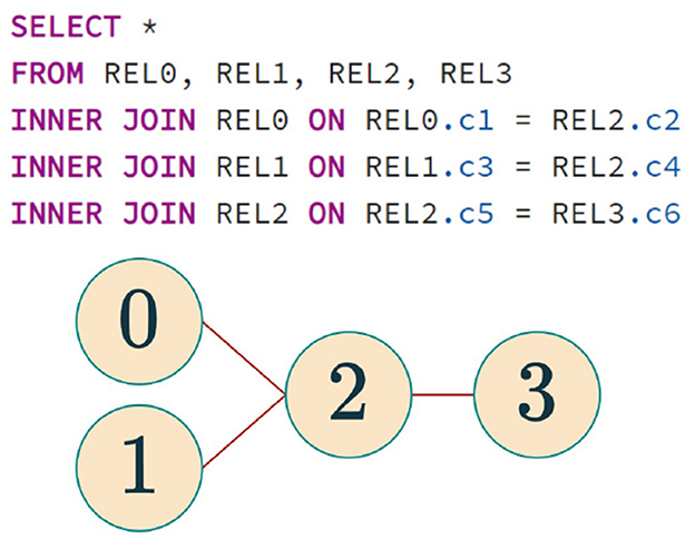
Figure 1. SQL query and its corresponding query graph. Each node represents a relation, and edges represent join predicates.

A join tree T of a query graph G is a binary tree in which each relation of G appears exactly once as a leaf node. Each internal node represents the join of its two children. For example, a non-leaf node labeled R_k1 ⋈ … ⋈ R_kn has two child subtrees, each of which contains a subset of the relations R_k1, …, R_kn. Following the definition in the study by Neumann and Radke (2018), we define that a join tree T adheres to a query graph G if for every subtree $T^{\prime }=T_1\bowtie T_2$ of T, there exists relations R₁ and R₂ such that R₁ ∈ T₁ and R₂ ∈ T₂ and (R₁, R₂) ∈ E. The join order selection problem is finding a join tree T that adheres to the query graph G and minimizes a given cost function. In this article, we refer to the requirement that a join tree adheres to the query graph as the validity constraint and the requirement of minimizing execution cost as the cost constraint. Next, we define the standard cost function for join trees.

Standard cost functions are based on estimating cardinalities of intermediate results in the join order selection process (Leis et al., 2015; Neumann and Gubichev, 2014; Cluet and Moerkotte, 1995). Thus, we first define how to compute the cardinality of a given join tree T. For a join tree T, its cardinality is defined recursively.

$\begin{array}{ll}\left|T\right|=\{\begin{array}{ll}\left|R_i\right|& \text{if }T=R_i\text{ is a leaf node,}\\ \left({\displaystyle {\prod }_{R_i\in T_1,R_j\in T_2}}{f}_{ij}\right)\left|T_1\right|\left|T_2\right|& \text{if }T=T_1\bowtie T_2.\end{array}& (1)\end{array}$

Based on the cardinalities, we define the cost function recursively as

$\begin{array}{ll}C(T)=\{\begin{array}{ll}0& \text{if }T=R_i\text{ is a leaf node,}\\ \left|T\right|+C(T_1)+C(T_2)& \text{if }T=T_1\bowtie T_2.\end{array}& (2)\end{array}$

This is the standard cost function (Cluet and Moerkotte, 1995), which has also been used in earlier quantum computing formulations (Schönberger et al., 2023a,b,c) and in the corresponding mixed-integer linear programming formulation (Trummer and Koch, 2017). More sophisticated cost models exist, whose integration into quantum optimization formulations will be part of future research.

In practice, two additional restrictions are common in join order optimization. First, query optimizers may avoid cross-product joins (also known as Cartesian products) because they produce large intermediate results. Unless explicitly required by the query graph, cross products are excluded from consideration. In our formulation, this differs from many previous quantum formulations, making our approach query-graph-aware. Second, optimizers often restrict the search space to left-deep join trees, where each join combines an intermediate result with a leaf relation. Left-deep trees dramatically reduce the search space compared to bushy join trees, where both join inputs can be intermediate results. Although bushy trees often yield lower costs, the blowup of the search space in possible plans makes them impractical for large queries. In this study, we follow these conventions and focus on left-deep join trees without cross products. It will be part of future research to include cross products, bushy trees, and more sophisticated cost functions.

2.2 Dynamic programming and greedy algorithms for join order selection

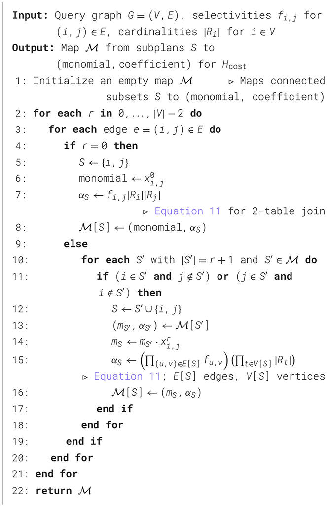
Our implementations of dynamic programming and greedy algorithms follow the study by Neumann and Gubichev (2014). They are well known and commonly used algorithms for join order selection (Selinger et al., 1979; Neumann and Radke, 2018; Moerkotte and Neumann, 2006, 2008). We present them in detail to build a clearer connection between them and the higher-order binary optimization formulation we develop in this work. Dynamic programming provides a general framework for systematically exploring possible join orders. In our study, we have fixed the cost function (Equation 2) and employed the dynamic programming algorithm with and without cross products. The algorithm without cross products is presented in Algorithm 1. It relies on functions that create left-deep trees for trees T₁ and T₂ and return costs for join trees based on the cost function in Equation 2.

Algorithm 1

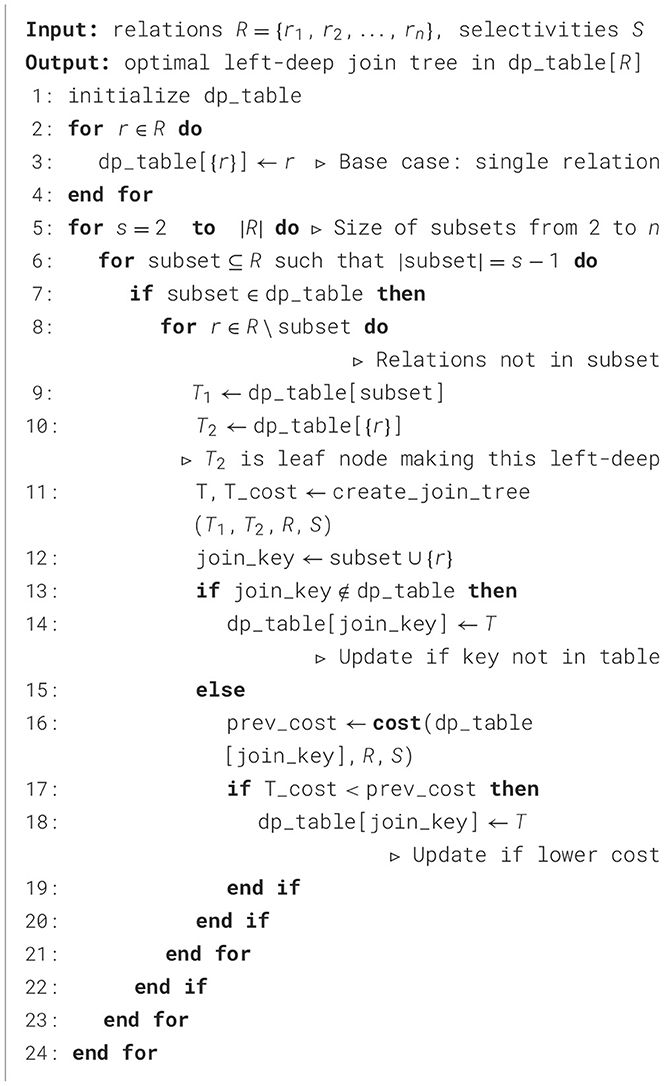
Algorithm 1. Dynamic programming for left-deep join order selection with cross products.

The algorithm that computes the dynamic programming result without cross products is similar, except that for a query graph G, we change line 6: for connected subgraph ⊂ G such that |subgraph| = s − 1 do. Then, the algorithm proceeds with the connected subgraphs of size s − 1, instead of all subsets of size s − 1.

The greedy algorithm is another standard algorithm for optimizing join order selection, as represented in Algorithm 2. Similar to the dynamic programming algorithm, we can consider only solutions without cross products so that we iterate only over relations connected to one of the relations already joined. In other words, at each step, we compute a value called adjacent_relations, which contains those relations R_i so that if edge (R_i, R_j) ∈ G in the query graph G, then R_i ∉ joined_relations but R_j ∈ joined_relations.

Algorithm 2

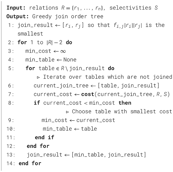
Algorithm 2. Greedy algorithm for left-deep join order selection with cross products.

2.3 Unconstrained binary optimization

Optimization is one of the key fields where quantum computing is assumed to provide computational value (Abbas and et al., 2024). This part provides a brief and high-level overview of how optimization algorithms are developed in quantum computing. We guide the reader to the study by Nielsen and Chuang (2010) and Winker et al. (2023b) for more detailed information about quantum computing. Additionally, the study by Schönberger et al. (2023a) provides an excellent introduction to quantum annealing and quadratic unconstrained binary optimization models for a database specialist.

Our study relies on higher-order unconstrained binary optimization (HUBO) (Boros and Hammer, 2002) problems, which are a generalization of quadratic unconstrained binary optimization (QUBO) problems. To the best of our knowledge, there is limited research on formulating domain-specific problems using HUBOs, which we will cover in more detail in the Discussion section. One reason for this is that HUBO problems are complex to solve not only theoretically but also practically (Boros and Hammer, 2002). Due to this computational complexity, they provide a potential area for exploring the practical benefits of quantum computing over classical approaches. Despite being challenging, they have a straightforward quantum computational formulation in theory (Verchere et al., 2023).

Next, we formally define HUBO problems (Boros and Hammer, 2002) and demonstrate their connection to QUBO problems. Let [n] = {1, …, n} be an indexing set. Let x ∈ {0, 1}ⁿ be a binary variable vector of type x = (x₁, …, x_n) so that x_i ∈ {0, 1} represents values false and true for each i ∈ [n]. The HUBO problem is the following minimization problem of a binary polynomial:

$\begin{array}{ll}{\displaystyle \underset{x\in {\left\{0,1\right\}}^n}{arg min}}{\displaystyle \sum _{S\subset [n]}}{\alpha }_S{\displaystyle \prod _{i\in S}}{x}_i,& (3)\end{array}$

where α_S ∈ ℝ. For each non-empty subset S, we have the corresponding higher-order term α_S ∏ _{i ∈ S} x_i. In practice, we might have α_S = 0 for many terms. In the worst case, we have 2ⁿ − 1 terms. Alternatively, we can write the same polynomial as

$\begin{array}{ll}{\displaystyle \sum _{S\subset [n]}}{\alpha }_S{\displaystyle \prod _{i\in S}}{x}_i={\displaystyle \sum _{i\in [n]}}{\alpha }_i{x}_i+{\displaystyle \sum _{i<j}}{\alpha }_{(i,j)}{x}_i{x}_j+{\displaystyle \sum _{i<j<k}}{\alpha }_{i,j,k}{x}_i{x}_j{x}_k+\dots & (4)\end{array}$

Quadratic unconstrained binary optimization (QUBO) problems are a restricted case of HUBO problems, where we consider only subsets of limited size, |S| ≤ 2. Concretely, a QUBO problem is the minimization problem of the polynomial.

$\begin{array}{ll}{\displaystyle \sum _{i\in [n]}}{\alpha }_i{x}_i+{\displaystyle \sum _{i<j}}{\alpha }_{(i,j)}{x}_i{x}_j.& (5)\end{array}$

Both QUBO and HUBO problems are NP-hard (Lucas, 2014; Boros and Hammer, 2002). As discussed, QUBO formalism has been the standard method for tackling database optimization problems, and many other wellknown optimization problems (e.g., knapsack, maxcut, and traveling salesman) have a QUBO formulation (Lucas, 2014).

2.4 Optimization on quantum hardware

Next, we provide a brief introduction to the basics of quantum computing for optimization problems and discuss techniques for solving HUBOs and QUBOs on quantum hardware. Quantum computing can be divided into multiple paradigms, both in terms of hardware and software. This division is exceptionally versatile, as there is no single “winning” method for building quantum computers yet. Quantum computers are designed to be built on superconducting circuits (IBM, Google, IQM) (Wendin, 2017), trapped ions (Quantinuum, IonQ) (Paul, 1990), neutral atoms (Quera, Pasqal) (Grimm et al., 2000), photons (Xanadu) (Knill et al., 2001), diamonds (Quantum Brilliance) (Neumann et al., 2008), and many other quantum mechanical phenomena (Gill et al., 2022). A special type of quantum hardware is a quantum annealer (D-Wave) (Apolloni et al., 1989; Kadowaki and Nishimori, 1998), which does not implement universal quantum computation but offers specific optimization capabilities for QUBO problems.

In addition to the hardware, a partially hardware-dependent software stack is designed to translate and compile high-level quantum algorithms into a format that specific quantum hardware supports. QUBOs are a widely accepted high-level abstraction that can be solved on most quantum hardware. The other common high-level abstraction is quantum circuits. Quantum algorithm design can still be divided into paradigms: adiabatic and circuit-based quantum computing, which are universal quantum computing paradigms (Aharonov et al., 2004). Unlike traditional introductions to quantum computing, we focus on the fundamentals of adiabatic quantum computing. This choice is motivated by the fact that our experimental evaluation was conducted on a quantum annealer, a type of adiabatic quantum computer.

Quantum computing can be implemented using the adiabatic evolution of a quantum mechanical system (Farhi et al., 2000; Mc Keever and Lubasch, 2024). This study uses quantum annealing, which is a part of the adiabatic quantum computing paradigm (Albash and Lidar, 2018). The evolution of a quantum mechanical system is governed by the Schrödinger equation (Nielsen and Chuang, 2010). This evolution models a system with a Hermitian operator known as a Hamiltonian. In this study, we are not interested in arbitrary Hamiltonians but in those with a form that maps to QUBO and HUBO optimization problems. For QUBOs, the corresponding problem Hamiltonian, also called an Ising Hamiltonian, is

$\begin{array}{ll}{\displaystyle \sum _i}{h}_i{\sigma }_z^i+{\displaystyle \sum _{j<i}}{J}_{i,j}{\sigma }_z^i{\sigma }_z^j,& (6)\end{array}$

where ${\sigma }_z^j$ are Pauli-Z operators for each j. The correspondence between the formulations in Equations 5, 6 is clear: the coefficients h_i and J_{i, j} represent the linear and quadratic terms, respectively. Operator ${\sigma }_z^i$ corresponds to the variable x_i for each i ∈ [n]. For HUBOs, the problem Hamiltonian is

${\displaystyle \sum _{S\subset [n]}}{\beta }_S{\displaystyle \prod _{i\in S}}{\sigma }_z^i,$

where the correspondence to Equation 4 is similar. As QUBO and HUBO problems are minimization problems, the goal is to find the minimum eigenvalue and eigenstate of the problem Hamiltonian. In other words, we aim to find a quantum state, called a ground state, where Hamiltonian's energy is minimized. As a result, we obtain a solution to the corresponding combinatorial optimization problem (Farhi et al., 2000).

Next, we describe how adiabatic quantum computing can find the lowest eigenstate and solve the optimization problem. For simplicity, let us focus on solving QUBOs on a quantum annealer. General adiabatic quantum computing is similar (Albash and Lidar, 2018). We define the following Hamiltonian (D-Wave Quantum Inc., 2025):

$\begin{array}{ll}H(s)={\displaystyle \underset{\text{initial Hamiltonian}}{{\displaystyle \underbrace{-\frac{A(s)}{2}{\displaystyle \sum _i}{\sigma }_x^i}}}}+{\displaystyle \underset{\text{problem Hamiltonian}}{{\displaystyle \underbrace{\frac{B(s)}{2}\left({\displaystyle \sum _i}{h}_i{\sigma }_z^i+{\displaystyle \sum _{j<i}}{J}_{i,j}{\sigma }_z^i{\sigma }_z^j\right)}}}},& (7)\end{array}$

where A(s) is the so-called tunneling energy function and B(s) is the problem Hamiltonian energy function at s. During the annealing process, the value s runs from 0 to 1, causing A(s) → 0 and B(s) → 1. We begin with a simple initial Hamiltonian, whose ground state is easily prepared, and gradually evolve it to the problem Hamiltonian. By the adiabatic theorem (Albash and Lidar, 2018), if the process is slow enough, the system remains in its ground state and ends up solving the optimization problem. However, quantum annealers are limited to solving QUBOs, meaning we cannot encode higher-order terms in the problem Hamiltonian. In contrast, universal adiabatic and gate-based quantum computers do not have this restriction in theory.

Using classical computers, we can solve QUBOs using simulated annealing (Kirkpatrick et al., 1983), digital annealing (Aramon et al., 2019), and classical solvers such as Gurobi and CPLEX. Unfortunately, classical solvers, such as quantum annealers, cannot natively solve higher-order binary optimization models; instead, we must rely on rewriting methods that reduce HUBOs to QUBOs. We introduce a reduction method to rewrite higher-order problems into quadratic ones. The key idea is to replace higher-order terms with slack variables. In this study, we primarily rely on the D-Wave Ocean framework's ability to automatically translate HUBO problems into QUBO problems. The HUBO to QUBO reduction based on minimum selection (D-Wave Quantum Inc, 2024) follows the scheme:

$\begin{array}{l}xyz={\displaystyle \underset{w}{max}}w(x+y+z-2),\end{array}$

where x, y, z, and w are binary variables. This method iteratively replaces the higher-order terms xyz with lower-order terms by introducing auxiliary binary variables w. Depending on the order in which variable terms are replaced, the QUBO formulation may vary in format and the number of binary variables, but the minimum point for the fixed HUBO remains unchanged.

3 Join order cost as HUBO

In this section, we develop two higher-order unconstrained binary optimization (HUBO) problems that encode the cost function (Equation 2) for left-deep join order selection problems. We will later focus on the validity constraint separately. Since validity will be built on the cost formulation, we present the cost formulation first. Compared to previous quantum computing research on join order optimization, we formulate the optimization problem from the perspective of joins, instead of relations (Schönberger et al., 2023a). This represents a new conceptual angle to the problem, which makes the formulations substantially distinct. The other new viewpoint is to encode the costs into coefficients of the HUBO polynomial, instead of encoding them with slack variables. This eliminates the need to estimate costs and use additional variables or qubits for encoding in the problem formulation.

The monomials in the HUBO formulation identify a specific join order path. The coefficients in the formulation describe the intermediate costs. Activating combinations of binary variables enables us to compute total join order costs for various join orders through activated monomials. Thus, the cost HUBO is the sum of terms, and we show that the minimum of the polynomial corresponds to the cost of the optimal plan.

Given a query graph G, the number of required joins to create a valid left-deep join tree is |V| − 1, where |V| is the number of nodes (i.e., relations or tables) in query graph G. This is easy to see since the first join is performed between two relations, and after that, every join includes one more relation until all the relations have been joined.

Our algorithm is designed to rank joins, and the ranking determines the order of the joins. This means a join (i.e., edge in the query graph G) has a rank 0 ≤ r < |V| − 1 if the join should be performed after all the lower rank joins are performed. We need |V| − 1 rank values to create a left-deep join order plan. Having |V| − 1 rank values applies to left-deep join plans but not bushy ones. For bushy plans, we can join multiple relations simultaneously, meaning that some of the joins can have the same rank, i.e., appear at the same level in the join tree. It will be part of future research to tackle these cases.

Initially, any join, i.e., edge (R_i, R_j) ∈ G, can have any rank 0 ≤ r < |V| − 1. Hence, we define the binary variables of our HUBO problems to be

$\begin{array}{ll}{x}_{i,j}^r\in \{0,1\},& (8)\end{array}$

where the indices i and j refer to the edge (R_i, R_j) ∈ G, where R_i and R_j are relations and r denotes the rank. Hence, our model consists of (|V| − 1)|E| binary variables since for every rank value 0 ≤ r < |V| − 1, we have |E| many joins (edges) from which we can choose the join.

The interpretation of these binary variables is as follows: If $x_{i,j}^r=1$, then the join (R_i, R_j) should be performed at rank r. Now the join (R_i, R_j) is not necessarily between the relations R_i and R_j since at r > 0, the left relation is an intermediate result of type R_k1 ⋈ … ⋈ R_i ⋈ … ⋈ R_kn for some indices k₁, …, k_n. Therefore, each tuple (R_i, R_j) represents a logical join predicate defined in the query graph, not a physical join operation in an execution plan.

Example 3.1. Consider that we have a simple, complete query graph of four relations {0, 1, 2, 3}. Thus, we have |V| = 4 relations, |E| = 6 possible joins, and (|V| − 1)|E| = 24 binary variables. Depending on the selectivities and cardinalities, an example solution that the model can return is $x_{0,1}^0=1$, $x_{1,2}^1=1$, and $x_{2,3}^2=1$, which gives us the left-deep join tree [[0, 1], 2], 3]. The solution is not unique; also, $x_{0,1}^0=1$, $x_{0,2}^1=1$, and $x_{2,3}^2=1$ produce the same plan with the same cost.

3.1 Precise cost function as HUBO

After defining the binary variables of our optimization model, we describe how to encode the cost function as a higher-order unconstrained binary optimization problem, whose minimum corresponds to the optimal cost up to cross products for the left-deep join order selection problem. We describe the cost constraint first, as the validity constraints can be computed based on terms that we derive for the cost constraint. First, we demonstrate the intuition behind the construction with an example.

Example 3.2. Every join should be performed at exactly one rank for left-deep join trees. Starting from rank 0, let us say that we choose to perform a join between the relations R₁ and R₂, obtaining R₁ ⋈ R₂. The corresponding activated binary variable is $x_{1,2}^0=1$. Based on the cost function in Equation 2, the cost of performing this join is f_{1, 2}|R₁||R₂|, where |R₁| and |R₂| are the cardinalities for the corresponding relations and f_{1, 2} is the selectivity. Thus, if we decide to make this join at this rank, we include the term

$\begin{array}{l}{f}_{1,2}|R_1||R_2|x_{1,2}^0\end{array}$

to the cost HUBO formulation. This example demonstrates that it is easy to encode the costs at rank 0, which correspond to linear variables in the cost HUBO.

Next, we assume the query graph gives us a join predicate with selectivity f_{2, 3} between the relations R₂ and R₃. Now we ask how expensive it is to perform the join between the intermediate result R₁ ⋈ R₂ and relation R₃. By Equation 2, the cost of making this join is

$\begin{array}{ll}{f}_{1,2}{f}_{2,3}|R_1||R_2||R_3|& (9)\end{array}$

assuming that there is no edge (R₁, R₃), which indicates that f_{1, 3} = 1 (Cartesian product). Note that this is not the total cost of performing all the joins but the cardinality of the resulting relation R₁ ⋈ R₂ ⋈ R₃. The left-deep join tree (R₁ ⋈ R₂) ⋈ R₃ should be selected if the following total cost function evaluates to a relatively small value.

$\begin{array}{l}{f}_{1,2}|R_1||R_2|x_{1,2}^0+f_{1,2}{f}_{2,3}|R_1||R_2||R_3|x_{1,2}^0{x}_{2,3}^1.\end{array}$

When the binary variables are active, i.e., $x_{1,2}^0=x_{2,3}^1=1$, the previous function evaluates the total cost of performing the join (R₁ ⋈ R₂) ⋈ R₃.

A key insight is that the cardinality in Equation 9 depends only on the set of relations being joined, not the order in which they were joined. In other words, this means that the cardinality in Equation 9 is the same for any join result that includes the relations R₁, R₂, and R₃, such as (R₁ ⋈ R₃) ⋈ R₂ and R₁ ⋈ (R₂ ⋈ R₃). This naturally generalizes to any number of relations. The total costs of these plans likely differ because intermediate steps have different costs. Intuitively, our HUBO model seeks the optimal configuration of joins to construct the full join tree, ensuring that the sum of the intermediate results is minimized.

Next, we formally describe the construction of the HUBO problem, which encodes the precise cost function for a complete left-deep join order selection problem that respects the structure of a given query graph G. The HUBO problem is recursively constructed with respect to the rank r. The construction of the HUBO problem becomes recursive because the definition of the cost function in Equation 2 is recursive.

Step r = 0. Let G = (V, E) be a query graph. By Equation 2, we include the costs of making the rank 0 joins to the cost HUBO. Thus, we add terms

$\begin{array}{l}|R_i\bowtie R_j|x_{i,j}^0=f_{ij}|R_i||R_j|x_{i,j}^0={\alpha }_{(i,j)}{x}_{i,j}^0,\end{array}$

for every join (R_i, R_j) ∈ E, where we denote α_{(i, j)}: = f_ij|R_i||R_j| as the coefficient encoding the cost.

Step r = 1. For clarity, we also show step r = 1. Assuming we have completed step r = 0, we consider adding variables of type $x_{i,j}^1$. For every join (R_i, R_j) ∈ E, we select the adjacent joins $(R_{i^{\prime }},R_{j^{\prime }})$ in the query graph. An adjacent join means that the joins share exactly one common relation. This creates quadratic terms of type $x_{i,j}^0{x}_{i^{\prime },j^{\prime }}^1$ with coefficients of type

${\alpha }_{(i,j,i^{\prime },j^{\prime })}^1:=f_{ij}{f}_{i^{\prime }{j}^{\prime }}{f}_{i^{\prime }j}{f}_{i{j}^{\prime }}|R_i||R_j||R_i^{\prime }||R_j^{\prime }|.$

So, we add terms ${\alpha }_{(i,j,i^{\prime },j^{\prime })}{x}_{i,j}^0{x}_{i^{\prime },j^{\prime }}^1$ to the cost HUBO.

Step for arbitrary r. Next, we consider adding a general rank 0 < r < |V| − 1 variables of form $x_{i^{\prime },j^{\prime }}^r$ to the HUBO problem. The construction can be divided into three steps:

1. We identify completed subplans. For this general case, we formalize the method using connected subgraphs of the query graph and the monomials consisting of the binary variables. Let $\mathcal{S}$ be the set of size r − 1 connected subgraphs in the query graph so that every subgraph corresponds to terms that were generated at step r − 1. The size of a subgraph is defined as the number of its vertices. Each such subgraph corresponds to a term that specifies a join order, resulting in an intermediate table containing exactly r − 1 relations. This means that the HUBO problem, encoding the total cost up to this step, has the following form:

$\begin{array}{l}{\displaystyle \underset{\text{case }r=0}{{\displaystyle \underbrace{{\displaystyle \sum _{(i,j)\in E}}{\alpha }_{(i,j)}{x}_{i,j}^0}}}}+{\displaystyle \underset{\text{case }r=1}{{\displaystyle \underbrace{{\displaystyle \sum _{(i,j)\in E}}{\displaystyle \sum _{(i^{\prime },j^{\prime })\in E}}{\alpha }_{(i,j,i^{\prime },j^{\prime })}{x}_{i,j}^0{x}_{i^{\prime },j^{\prime }}^1}}}}+\dots \\ +{\displaystyle \underset{\text{case }r-1}{{\displaystyle \underbrace{{\displaystyle \sum _{S\in \mathcal{S}}}{\alpha }_S{\displaystyle \prod _{(R_i,R_j)\in S,0\le k\le r-1}}{x}_{i,j}^k}}}}.\end{array}$

2. We construct the new HUBO monomials for rank r. For simplicity, we first focus on generating the next term without a coefficient α. Let $S\in \mathcal{S}$ be a fixed subgraph of the query graph. Let $(R_{i^{\prime }},R_{j^{\prime }})\in E$ be an edge that is not part of the subgraph S but connected to it so that either $R_{i^{\prime }}\in S$ or $R_{j^{\prime }}\in S$ (but not both $R_{i^{\prime }},R_{j^{\prime }}\in S$). This means we join exactly one new relation. For this fixed subgraph S and fixed join $(R_{i^{\prime }},R_{j^{\prime }})$, we are going to add the following element to the cost HUBO:

$\begin{array}{ll}{\displaystyle \underset{\text{term at rank }r-1}{{\displaystyle \underbrace{{\displaystyle \prod _{(R_i,R_j)\in S,0\le k\le r-1}}{x}_{i,j}^k}}}}{\displaystyle \underset{\text{new variable at rank }r}{{\displaystyle \underbrace{x_{i^{\prime },j^{\prime }}^r}}}}& (10)\end{array}$

The new term is just the “old” term from the previous step multiplied by the new variable $x_{i^{\prime },j^{\prime }}^r$.

3. We compute the coefficient for the new monomial. A coefficient in the HUBO formulation represents a cardinality of the intermediate relation formed by the set of joins encoded in the corresponding monomial. Consider the new induced subgraph $S^{\prime }=S\cup \left\{(R_{i^{\prime }},R_{j^{\prime }})\right\}$. The new coefficient ${\alpha }_{S^{\prime }}$ is easy to compute based on the subgraph S and the latest included join $(R_{i^{\prime }},R_{j^{\prime }})$. Note that the induced subgraph S′ may contain new edges besides the latest included edge $(R_{i^{\prime }},R_{j^{\prime }})$. However, the new coefficient for term (Equation 10) is

$\begin{array}{ll}{\alpha }_{S^{\prime }}={\displaystyle \prod _{(R_i,R_j)\in S^{\prime }}}{f}_{i,j}{\displaystyle \prod _{R_i\in S^{\prime }}}\left|R_i\right|.& (11)\end{array}$

This formula is the general expression of Equation 9 in Example 3.2.

This recursive process is repeated until we reach rank r = |V| − 2, at which point the generated monomials will represent all possible valid, complete left-deep join trees. The full cost HUBO is the sum of all terms generated at all ranks from 0 to |V| − 2. The idea of how the terms are appended at rank 2 is visualized in Figure 2. One of the final configurations is visualized in Figure 3, which also shows how the terms are interpreted as join trees.

Figure 2

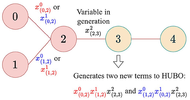
Figure 2. With relations 0, 1, and 2 already joined, relation 3 is the only option for left-deep plans. Two combinations arise based on whether edge (0, 2) or (1, 2) joins first. Coloring links graph variables to the monomials in HUBO.

Figure 3

Figure 3. One option as the final assignment for the binary variables in the query graph. The algorithm returns the corresponding join tree if the variables are selected as true. Coloring links between graph variables and the monomials in HUBO, as well as to the generated plan.

The concrete algorithm for generating the cost HUBO is presented in Algorithm 3. It inputs a query graph and outputs the cost HUBO. The keys in this dictionary are sets of relations, and the values are tuples consisting of a monomial and its coefficient, which define the HUBO polynomial for the problem.

Algorithm 3

Algorithm 3. Construct monomials and coefficients for precise cost HUBO.

3.2 Encoding heuristic cost function as HUBO

While this formulation for the precise cost function is exact, its computational complexity grows rapidly. Therefore, a heuristic approach is often necessary. Thus, we have modified the generation of the cost function to include a greedy heuristic in the HUBO construction process (Algorithm 3) to include only those higher-order terms that are likely to introduce the least cost to the total cost function.

The idea behind the heuristic is the following: First, we again include all the rank 0 terms. When we start including rank 1 terms, we consider only those rank 0 terms whose cardinality (i.e., the coefficient α_{(i, j)} in the HUBO objective) is minimal. We have included a tunable hyperparameter n that selects n terms with the smallest coefficients. Then, the HUBO construction continues with the selected subset of terms. With this heuristic, the size of the optimization problem is reduced remarkably, although we lose the guarantee of finding the optimal plan.

This heuristic is implemented by modifying Algorithm 3. Specifically, in line 7, instead of iterating over all subplans from the previous rank, we select only the top-n subplans with the smallest associated cost coefficients. In other words, we change line 7 to be “n many relations associated with the rank r − 1 variable with the smallest coefficients”. We will later prove that this formulation produces at least as good a plan as the classical greedy algorithm and likely produces better plans for larger values of n. For sufficiently large n, this formulation reduces back to the first, precise cost HUBO formulation.

4 Join order validity as HUBO

For a HUBO formulation to be effective, its objective function must be constructed so that the minimizing point also represents a valid solution. In this case, validity refers to the join tree's adherence to the query graph, as defined in the Background section. All valid solutions are usable, although they might not minimize the cost. In this section, we present two approaches to encoding the validity of solutions: cost function-dependent and cost function-independent. A cost function-dependent approach is easy to construct but produces a larger number of higher-order terms. The cost function-independent approach is closer to the standard QUBO formulations and identifies a set of constraints that the formulation must satisfy. The advantage of the second formulation is that its terms are primarily quadratic, which makes it easier to optimize in practice.

4.1 Cost function-dependent validity

Considering the cost HUBO generation in the previous section, we have generated higher-order terms that encode valid join trees at rank r = |V| − 2. After applying Algorithm 3, we can access these terms with $\mathcal{M}[V]$, where the set V is the node set, i.e., the set of relations. Let us denote this set of terms as $H:=\mathcal{M}[V]$. For example, one of the terms is represented in Figure 2. The first validity constraint forces the model to select exactly one of these terms as true, which ensures that the final join tree contains all the relations.

4.1.1 Select one valid plan

We use a generalized one-hot (or k-hot) encoding from QUBO formulations (Lucas, 2014; Schönberger et al., 2023c). The encoding constructs a constraint that reaches its minimum when precisely k variables are selected to be true from a given set of binary variables. In the generalized formulation, we construct an objective that is minimized when exactly k terms are selected as true from a set of higher-order terms. Let H be the set of higher-order terms at rank r = |V| − 2. This functionality generalizes to higher-order cases with the following formulation:

$\begin{array}{ll}{\left(1-{\displaystyle \sum _{h\in H}}h\right)}^2,& (12)\end{array}$

where $h={\prod }_{r=0}^{\left|V\right|-2}{x}_{i_r,j_r}^r$ for some indices i_r and j_r for r = 0, …, |V| − 2 that depend on the query graph. This polynomial is minimized at a value of 0 if and only if exactly one term h in the summation is equal to 1, thereby enforcing the selection of a single valid plan. A detailed proof is provided in the theoretical analysis section.

4.1.2 Every rank must appear exactly once in the solution

A challenge with this approach is that the model may produce solutions containing unnecessarily activated variables. For example, a variable x might be set to 1, but if it only appears in terms where another variable is 0 (e.g., xy, where y = 0), its activation has no impact on the final cost. Consider the plan in Figure 2. The HUBO that encodes this plan would have the same minimum even if we set $x_{0,2}^1=1$ because this variable would always be multiplied by variables set to 0. While this can be solved with classical post-processing, and it does not affect the theoretical construction, we address it with an additional constraint. We include a constraint that every rank should appear exactly once in the solution. This is also an instance of one-hot encoding (D-Wave Systems Inc., 2024) and encoded with the following quadratic objective:

$\begin{array}{ll}{\displaystyle \sum _{r=0}^{\left|V\right|-2}}{\left(1-{\displaystyle \sum _{(R_i,R_j)\in E}}{x}_{i,j}^r\right)}^2.& (13)\end{array}$

The objective H₁ is minimized when exactly one variable of type $x_{i,j}^r$ is selected to be true for each 0 ≤ r < |V| − 1. This constraint enforces the fundamental rule of left-deep plans: At each rank r, exactly one join must be selected. The inner summation counts the number of joins selected at rank r. The expression is minimized to 0 when this count is exactly 1, thus providing a constraint for each rank.

4.2 Cost function-independent validity

The validity constraint in Equation 12 produces higher-degree terms due to exponentiation to the power of two, which we might want to avoid. Hence, we develop join tree validity constraints independently from the cost function. Notably, these validity constraints are often quadratic, i.e., QUBOs, and are automatically supported by many solvers. Because we develop the theory considering the query graph's structure, we have slightly different constraints depending on the query graphs.

4.2.1 Clique graphs

Every rank must be selected exactly once in the solution. This first constraint was already presented in Equation 13.

Select connected join tree. The second constraint encodes that we penalize cases that do not form a connected join tree. To achieve this, we include a constraint of the following form:

$\begin{array}{ll}{\displaystyle \sum _{r=0}^{\left|V\right|-2}}{\displaystyle \sum _{(i,j)\in E}}{\displaystyle \sum _{(i^{\prime },j^{\prime })\in E}}C{x}_{i,j}^r{x}_{i^{\prime },j^{\prime }}^{r+1},& (14)\end{array}$

where we sum over the elements if the indices satisfy |{i, j} ∩ {i′, j′}| ≠ 1. This constraint penalizes two types of invalid sequences: (1) selecting the same join at two consecutive ranks and (2) selecting two joins at consecutive ranks that share no common relations. This encourages the model to select a new join that connects to the existing intermediate result, forming a connected graph.

Result contains all the relations. The third constraint forces us to join all the relations. Our framework identifies joins as pairs of relations (R_i, R_j). This leads to one relation R_i appearing multiple times in variables, referring to different joins in a valid solution. An example of this is presented in Figure 3, where relation 2 appears multiple times in the solution, consisting of joins such as (0, 2) and (1, 2). This third constraint encodes that we count the number of relations and require that the count is at least one for each relation. Counting relations involves a minimum of a logarithmic number of slack variables (the method to do the logarithmic encoding is presented in Lucas, 2014) in terms of relations. For technical simplicity, we present the less efficient but equivalent method here:

$\begin{array}{ll}{\displaystyle \sum _{R_i\in G}}{\left(1+{\displaystyle \sum _{k=2}^{\left|V\right|-2}}k{y}_k^i-{\displaystyle \sum _i}{\displaystyle \sum _{r=1}^{\left|V\right|-2}}{x}_{i,j}^r\right)}^2.& (15)\end{array}$

The constraint reaches zero if at least one variable of type $x_{i,j}^r$ is true for each relation R_i. The constraint ensures that each relation R_i is included in at least one selected join. It uses slack variables $y_k^i$ to encode the count of how many times a relation appears in the plan, penalizing cases where the count for a given relation is zero.

4.2.2 Chain, star, cycle, and tree graphs

At every rank, we have performed rank + 1 many joins. This constraint is related to the first validity constraint presented in the study by Schönberger et al. (2023a) and Schönberger et al. (2023b). They present the constraint in terms of relations, whereas we have constructed it in terms of joins. The constraint encodes the number of joins we must perform cumulatively at each rank. In other words, when the rank is 0, we select one variable of type $x_{i,j}^0$ to be true. When the rank is 1, we choose two variables of type $x_{i,j}^1$ to be true. Formally, this constraint is

$\begin{array}{ll}{\displaystyle \sum _{r=0}^{\left|V\right|-2}}{\left(r+1-{\displaystyle \sum _{(i,j)\in E}}{x}_{i,j}^r\right)}^2.& (16)\end{array}$

The constraint is minimized at 0 when for each 0 ≤ r < |V| − 1, we have selected exactly r + 1 variables of type $x_{i,j}^r$ to be true.

Include the previous joins in the proceeding ranks. This constraint is again similar to the second constraint presented in the study by Schönberger et al. (2023a) and Schönberger et al. (2023b), except that we express the constraint using joins. If the join happened at rank r, it should be included in every proceeding rank ≥ r. In other words, we retain the information from the performed joins for subsequent ranks. This can be achieved with the following constraint:

$\begin{array}{ll}{\displaystyle \sum _{(i,j)\in E}}{\displaystyle \sum _{r=1}^{\left|V\right|-2}}{x}_{i,j}^{r-1}(1-x_{i,j}^r).& (17)\end{array}$

Now, if $x_{i,j}^{r-1}$ is active, then the model favors the case that $x_{i,j}^r$ is active too since in that case, $1-x_{i,j}^r=0$. If $x_{i,j}^r=0$, the term evaluates to 1, which penalizes the configuration.

Respect query graph: chain, star, cycle. Since the cost functions are designed to respect structures of query graphs, we use the following constraint to encode the graph structure in chain, star, and cycle graphs:

$\begin{array}{ll}{\displaystyle \sum _{r=0}^{\left|V\right|-1}}{\displaystyle \sum _{(i,j)\in E}}{\displaystyle \sum _{(i^{\prime },j^{\prime })\in E}}-C{x}_{i,j}^r{x}_{i^{\prime },j^{\prime }}^r,& (18)\end{array}$

where |{i, j} ∩ {i′, j′}| = 1, which means that the joins have to share exactly one relation. Setting the coefficient −C as negative, we favor the cases when the joins share precisely one relation. This constraint is complementary to the constraint in Equation 14.

Respect query graph: tree. Unfortunately, the previous constraint fails to encode the minimum for certain proper trees that contain nodes with at least three different degrees. The simplest, problematic tree shape is represented in Figure 3 (node 2 has degree 3, node 3 has degree 2, and the others have degree 1). The problem is that with the constraint in Equation 18, not all the join trees have the same minimum energy due to the different degrees of the nodes. To address this problem, we develop an alternative constraint:

$\begin{array}{ll}{\displaystyle \sum _{r=1}^{\left|V\right|-1}}{\left(r-{\displaystyle \sum _{(i,j)\in E}}{\displaystyle \sum _{(i^{\prime },j^{\prime })\in E}}{x}_{i,j}^r{x}_{i^{\prime },j^{\prime }}^r\right)}^2,& (19)\end{array}$

where again we form the sum over the elements if the indices satisfy |{i, j} ∩ {i′, j′}| = 1. At every rank, this constraint selects r-many pairs of type $x_{i,j}^r{x}_{i^{\prime },j^{\prime }}^r$ to be true. This forces the returned join tree to respect the query graph and be connected. This constraint is slightly more complex than the previous constraints, as it is not quadratic but a higher-order constraint that includes terms involving four variables. On the other hand, it does not introduce additional variables.

Total HUBO and scaling cost and validity constraints. Finally, the cost HUBO and the validity encoding HUBO are summed together. Validity constraints are added to the objective function with a large penalty coefficient C > 0. The penalty C must be sufficiently large to ensure that any violation of the validity constraints creates a penalty larger than any potential savings in the cost function. This ensures that the cost H_cost and the validity objective H_val are scaled properly so that the model favors valid solutions over minimizing cost:

$H_{\text{full}}=H_{\text{cost}}+C{H}_{\text{val}}.$

A possible heuristic is to set C to be greater than the maximum value of H_cost. We found that setting C to the sum of all positive coefficients in H_cost worked consistently in our experiments.

5 Theoretical analysis

This section proves two theorems that provide bounds for the quality of the solutions that can theoretically be achieved with the proposed HUBO formulations for the join order selection problem. We introduced the classical baseline algorithms in Algorithms 1, 2. We emphasize that the HUBO formulations and the proofs are constructed to respect the underlying query graph. This means that the algorithms assume that cross products are expensive and could be avoided. Beneficial cross products can be explicitly encoded by adding an edge to the query graph with a selectivity of 1, and the proofs apply to cases with cross products by considering clique graphs where some of the selectivities are 1. While our formulation does not automatically discover such cross products, it can optimize them if they are provided, and this is a promising direction for future research.

By the definition of binary variables in Equation 8, we can prove the theorems by induction on the rank parameter r in the proposed HUBO constructions, as well as the iterations in the dynamic programming and greedy algorithms. Our proof strategy is to show that for every plan considered by the classical algorithms, there is a corresponding assignment in our HUBO formulation with the same cost, such that this assignment is also a minimizing solution to the HUBO problem.

Lemma 1. Let G = (V, E) be a query graph and let x ∈ {0, 1}^{|V| − 1} be a binary vector. Let H_val be the validity constraint consisting of constraints in Equations 12, 13. If the cost-dependent validity constraint evaluates H_val(x) = 0, then vector x encodes a valid left-deep plan.

Proof. First, assume that the cost-dependent validity constraint evaluates H_val(x) = 0. The first constraint in Equation 12 is

$\begin{array}{ll}{\left(1-{\displaystyle \sum _{h\in H}}h\right)}^2,& (20)\end{array}$

where $h={\prod }_{r=0}^{\left|V\right|-2}{x}_{i_r,j_r}^r$ for some indices i_r and j_r for r = 0, …, |V| − 2 that depend on the query graph. This constraint is always non-negative since it is squared. It is positive, except when exactly one of the terms in the sum $\sum _{h\in H}h$ is 1 when the constraint evaluates to 0. The sum $\sum _{h\in H}h$ evaluates to 1 when there is exactly one term h such that all the variables in the product $h={\prod }_{r=0}^{\left|V\right|-2}{x}_{i_r,j_r}^r$ are true. This combination of activated variables is the valid join tree that the objective function returns as a solution to the minimization problem.

By construction of H (Algorithm 3), every monomial h ∈ H encodes a left-deep sequence since

• The construction starts from a single edge at rank 0.

• At rank r > 0, the construction extends the previously accumulated connected subgraph (plan) by one edge (join) that is incident to it, thereby adding exactly one new relation.

• The construction reaches a subgraph whose vertex set is V at rank |V| − 2.

These features define a valid left-deep plan. Therefore, the unique x selected above maps to a valid left-deep join plan that respects the query graph G.

Lemma 2. Let G = (V, E) be a query graph and let x ∈ {0, 1}^{|V| − 1} be a binary vector. If the cost-independent validity constraint evaluates H_val(x) = 0, then x encodes a valid left-deep plan.

Proof. We divide the proof into two parts depending on the structure of the query graph.

Clique graphs. In the case of clique graphs, the used validity constraints are as follows.

1. There is precisely one join per rank, which is encoded with the constraint in Equation 13.

2. Consecutive joins must share exactly one relation and must not be identical or disjoint, which was encoded with the constraint in Equation 14.

3. Every relation appears at least once across all ranks, encoded in Equation 15.

Assume that the cost-independent validity constraint evaluates H_val(x) = 0. Since every constraint is non-negative, this means that they have to evaluate to 0. The first point ensures that there are exactly |V| − 1 edges, and the second point ensures that the graph is connected. Thus, it is a tree. The last point ensures that every relation appears in the tree, and thus, it is a valid join tree.

The previous constraints are sufficient to also encode a left-deep join tree without additional constraints. For r = 0, the subgraph S₀ contains two relations. The join e_{r + 1} at rank r + 1 must connect to the join e_r at rank r by the constraint in Equation 14. Since the overall graph of joins is a tree, adding e_{r + 1} cannot form a cycle with the previously selected joins. This implies that e_{r + 1} must connect exactly one new relation to the set of relations S_r. Therefore, this progressive inclusion of exactly one new relation at each step defines a left-deep join plan.

Chain, star, cycle, and tree graphs. In this case, the used validity constraints are as follows:

1. We have a cumulative cardinality: at rank r, exactly r + 1 join variables are active, which is encoded by the constraint in Equation 16.

2. Join variables propagate across ranks: Once a join becomes active, it remains active, encoded in the constraint in Equation 17.

3. Enforce the correct adjacency at each rank. This is encoded with the constraints in Equations 18, 19.

Define $A_r=\left\{(i,j)\in E\mid x_{i,j}^r=1\right\}$ for each 0 ≤ r ≤ |V| − 1. Assuming the previous points and H_val(x) = 0, we obtain A₀ ⊂ A₁ ⊂ ⋯ ⊂ A_{|V| − 2}. From the first point, it follows that |A_r| = r + 1, and the second point ensures that A_{r − 1} ⊂ A_r. Thus, exactly one new join is added at each step. Moreover, the unique new join added when passing from A_{r − 1} to A_r shares exactly one endpoint with the current result.

Next, we consider the structure. For chain, star, and cycle queries, Equation 18 gives a negative reward for each pair of same-rank joins that share exactly one endpoint. Summing over all pairs at rank r forces A_r to be a single connected component because disconnected elements are penalized. For proper trees, the constraint in Equation 19 enforces exactly r adjacent pairs among the possibilities. That is a characterization of a tree on r + 2 vertices with r + 1 edges, which makes A_r connected and acyclic.

Since |A_r| = r + 1 and A_r is connected, it defines a tree. Since A_r = A_{r − 1} ∪ {e_r} and A_{r − 1} is connected and acyclic, the only way how A_r is a tree is that the edge e_r shares exactly one endpoint with A_{r − 1}. This indicates that the plan is left-deep.

Theorem 3. Let G = (V, E) be a query graph. Define binary variables $x_{i,j}^r\in \left\{0,1\right\}$ for each rank r ∈ {0, …, |V| − 1} and join edge (i, j) ∈ E as we defined in the context of binary variables in Equation 8. Let H_cost be the precise HUBO formulation obtained by Algorithm 3 with the coefficients given by Equation 11. This means that every rank-r term corresponds to extending a connected subgraph by one adjacent edge and carries the cardinality-based cost contribution defined in Equation 1. Let H_val be any of the validity encodings in Section 4. Consider

$H_{\text{full}}:=H_{\text{cost}}+C{H}_{\text{val}},$

with a constant C > 0 chosen so that valid solutions are always preferred to any invalid ones. Let x^⋆ minimize H_full. Then, the solution x^⋆ encodes a valid left-deep plan T^⋆ without cross products whose cost equals the cost from the DP algorithm without cross products:

$H_{\text{cost}}(x^{\star })=C(T^{\star }),$

where C(·) is the recursive cost in Equation 2.

Proof. The proof consists of three parts, which ensure the optimality and correctness: a bijection between valid DP plans and assignments without penalty, a rank-wise construction which identifies costs from H_cost with costs in the DP table, and penalty scaling to enforce feasibility.

1. Based on Lemma 1 and Lemma 2, it suffices to show that the set

$\begin{array}{ll}\left\{T\mid T\text{ is a left-deep plan adhering }G\right\}& (21)\end{array}$

is in a bijective relationship with the set

$\begin{array}{ll}\left\{x\mid H_{\text{val}}(x)=0\right\}.& (22)\end{array}$

Every left-deep plan T can be written as a sequence of joins (e₁, e₁, …, e_{|V| − 1}), where each e_r = (i_r, j_r) ∈ E joins exactly one new relation to the current connected join tree, and the join tree T adheres to the query graph G in the sense of Subsection 2.1. Define a mapping ϕ:T → {0, 1}^{|V| − 1} by

$\varphi (e_r)=x_{i,j}^r=\{\begin{array}{c}1(i,j)=e_r,\\ 0\text{otherwise}.\end{array}$

By construction, the image ϕ(T) = x satisfies the following properties:

• There is exactly one active variable at each rank r ∈ [1, |V| − 1], which is forced by the constraint in Equation 13.

• Consecutive joins share exactly one relation and extend connectivity, which is encoded with the constraint in Equation 14.

• All the relations appear in the solution, which is encoded with the constraint in Equation 15.

• Only edges (i.e., joins) in E are used, so there are no cross products. We called these constraints respecting the query graph G, and they were encoded in Equations 18, 19.

Since this means that for the element ϕ(T) = x every constraint is satisfied, we obtain that H_val(x) = 0. Conversely, for any x for which H_val(x) = 0, the previous constraints are satisfied, which means that exactly one join per rank is activated, and we obtain a connected left-deep sequence of edges in E. This decodes a plan T = ϕ⁻¹(x). Thus, we obtain the bijection between sets in Equations 21, 22.

2. Next, we define a rank-wise invariant, which is proved to preserve the join order cost. The DP algorithm (without cross products) maintains, at iteration r, the DP table, which records all connected subplans with r + 1 relations. It also stores for each subplan its total cost under the cost function in Equation 2. Then, there exists an invariant I(r) as follows. After Algorithm 3 has generated all terms up to rank r, for every connected subplan S with |S| = r + 1, there exist a set of variables ${\left\{x_{i_k,j_k}^k\right\}}_{k=0}^r$ such that

1. The product term created by Algorithm 3 for S,

${\displaystyle \prod _{k=0}^r}{x}_{i_k,j_k}^k,$

is part of H_cost, and

2. the sum of coefficients contributed along this product (with αs from Equation 11) equals the DP total cost of S, i.e., the cumulative sum of intermediate cardinalities described by the cost function in Equation 2. Particularly, activating exactly these r + 1 variables yields H_cost equal to the DP table entry for S.

Proof of the invariant. First, we consider the base case, when r = 0. By Algorithm 3, all the joins between the leaf relations are included in the cost function H_cost: α_{(i, j)} = f_{i, j}|R_i||R_j|, which is exactly the DP cost of that binary join. Thus, I(0) holds.

Inductive step. Assume that I(r − 1) holds. This means that there exists a connected subgraph S_prev of size r. Fix a connected subplan S of size r + 1. By construction, Algorithm 3 forms S by extending S_prev with an adjacent edge (i′, j′) ∈ E that adds exactly one new relation. The new coefficient attached to this extension is α_S, which is computed with Equation 11. This is precisely the cardinality, i.e., cost for the intermediate result after adding the (i′, j′) join. Summing this with the previously accumulated coefficients for S_prev, which exists by the induction assumption, gives exactly the DP total cost for S. Hence, I(r) holds.

Thus, for any left-deep plan T and x = ϕ(T), when applying I(|V| − 2), we obtain

$\begin{array}{ll}{H}_{\text{cost}}(x)=C(T).& (23)\end{array}$

3. Finally, we consider optimality under the penalty constraint. We choose the constant C so that any violation of the validity constraint H_val raises the objective by at least the maximum possible variation of H_cost. Since every term in H_cost is positive, the simple choice for this is C: = H_cost(1), where 1 = (1, …, 1). Then, any minimizer x^⋆ of H_full must satisfy $H_{\mathrm{\text{val}}}(x^{\star })=0$. This means that x^⋆ is valid and corresponds to some left-deep plan T^⋆, which we showed earlier.

Among such valid assignments, minimizing H_full becomes identical to minimizing H_cost. Restricting to valid x = ϕ(T) gives H_cost(x) = C(T), as we pointed out in Equation 23. Therefore, x^⋆ encodes a plan T^⋆ whose cost is minimal among all left-deep plans without cross products. This is exactly the DP optimum without cross products: $H_{\mathrm{\text{cost}}}(x^{\star })=C(T^{\star })$. This finalizes the proof.

Theorem 4. Let H_cost be the heuristic method's cost HUBO defined in subsection 3.2. Let x^⋆ be a minimizer of H_cost. Then, H_cost(x) ≤ C_greedy, i.e., the cost from the greedy algorithm gives an upper bound for the cost from the heuristic algorithm.

Proof. We use the same rank index r ∈ [0, |V| − 2] as in the previous theorem, and use the same cost–coefficient mapping defined in Equation 11. We again prove an invariant with respect to r as follows.

Invariant: For each rank r, the greedy algorithm's partial plan, T_r, is contained within the set of partial plans (the frontier) maintained by the heuristic HUBO construction.

Base case (r = 0): The heuristic algorithm includes all leaf joins at rank 0, so it contains the cheapest leaf join chosen by the classical greedy algorithm.

Inductive step: Assume the invariant holds for rank r − 1, meaning T_{r − 1} is in the heuristic's frontier. The greedy algorithm extends T_{r − 1} by selecting the adjacent relation that minimizes the local cost increment. According to Equation 11, these local increments are precisely the α-coefficients for the valid rank-r extensions of T_{r − 1} in the HUBO formulation.

At rank r, the heuristic selects the top extensions based on the smallest coefficients. Since the greedy choice corresponds to the extension with the smallest increment (and thus smallest coefficient), it is guaranteed to be selected by the heuristic. Thus, the partial plan T_r is included in the heuristic's frontier, completing the induction.

Because the heuristic frontier contains the entire greedy path T₀, …, T_{|V| − 2} and the HUBO objective function sums the same local increment that the greedy algorithm accumulates along that path, there exists a feasible assignment x′ whose value equals the cost C_greedy from the classical greedy algorithm. The minimizer x^⋆ of H_cost among valid plans cannot therefore do any worse, and we obtain

$\begin{array}{l}{H}_{\text{cost}}(x)\le H_{\text{cost}}(x^{\prime })=C_{\text{greedy}}.\end{array}$

5.1 Complexity analysis

Here, we consider the computational complexities of the proposed algorithms. The join order problem with the cost model in Equation 2 is generally NP-hard (Cluet and Moerkotte, 1995). The time complexity of dynamic programming algorithm depends on the query graph, the type of the dynamic programming algorithm, the type of the returned join plan (left-deep, zigzag, bushy, etc.), and whether cross products are included (Moerkotte and Neumann, 2006). The computational complexity ranges from O(3^|V|) to linear. More precisely, the dynamic programming algorithm in this work is based on Algorithm 1. The complexity analysis of this algorithm shows that the worst-case running time is O(2^|V|) for clique graphs (Neumann and Gubichev, 2014). Note that this is for left-deep trees, whereas the similar algorithm for finding bushy plans has complexity O(3^|V|) (Neumann and Gubichev, 2014).

Similarly, the time complexity of the greedy algorithm in Algorithm 2 depends on the structure of the query graph. The algorithm first evaluates the join between every pair of relations with respect to the query graph, requiring at most O(|V|²) steps. The greedy algorithm continues to evaluate the current cheapest plan with all the relations, which leads to a final time complexity of O(|V|²).

The complexity of solving HUBO and QUBO-based problems on quantum and classical hardware can be divided into multiple steps. The HUBO and QUBO problems are theoretically NP-complete problems (Lucas, 2014; Boros and Hammer, 2002). In practice, their difficulty also depends on the number of variables, the number of terms, the degree of the terms, the range of the coefficients, and how close the ground state is to the first excited state. For this HUBO formulation, the degree of the terms is at most the number of relations in the query. The cardinalities and selectivities of the relational database instance fully define the range of the coefficients. In the following, we will analyze the number of variables and the number of terms relying on the description of Algorithm 3.

5.1.1 Complexity of HUBO construction

The complexity of Algorithm 3 depends on the query graph. The outer loop over ranks runs for r = 0, …, |V| − 2. When r = 0, the algorithm performs |E| steps. When r > 0, the algorithm performs the following. Let $\left|{\mathcal{H}}_r\right|$ denote the set of all connected subgraphs with exactly r + 1 vertices at rank r. At each rank r > 0, the algorithm loops over all |E| edges, and for each edge, iterates over the set of partial plans in ${\mathcal{H}}_{r-1}$ to test whether the edge can extend the subplan by one relation. Each such check and possible extension costs O(1) time. Hence, the total runtime is

$O\left(|E|+{\displaystyle \sum _{r=1}^{\left|V\right|-1}}\left|E\right|·|{\mathcal{H}}_r|\right)=O\left({\displaystyle \sum _{r=0}^{\left|V\right|-1}}\left|E\right|·|{\mathcal{H}}_r|\right).$

Thus, we see that the total performance depends on the growth of the term $\left|{\mathcal{H}}_r\right|$. Worst-case complexity is achieved in a clique query graph, where every subset of r + 1 vertices forms a connected subgraph, so $\left|{\mathcal{H}}_r\right|=\left(\genfrac{}{}{0.0pt}{}{\left|V\right|}{r+1}\right)$. Substituting into the bound above gives

$O\left(|E|·2^{\left|V\right|}\right)=O\left(|V{|}^2·2^{\left|V\right|}\right).$

Thus, Algorithm 3 has exponential time complexity in the worst case, which matches the combinatorial complexity of the dynamic programming algorithm for join-order selection.

For other query graphs, the number of connected subsets is smaller. It is sufficient to consider only subtrees since Algorithm 3 enumerates only connected subgraphs that are left-deep plans, which are trees. It was proved that the number of subtrees for chains is $\left(\genfrac{}{}{0.0pt}{}{\left|V\right|+1}{2}\right)$ and the number of subtrees for star graphs is O(2^|V|) (Székely and Wang, 2005). This leads to the complexity result that the number of subgraphs grows as O(|V|²) for chain graphs, which in turn yields a time complexity of O(|V|³) since |E| = |V| − 1. For the star graphs, we have |E| = |V| − 1 and thus obtain complexity O(|V| · 2^|V|), which also aligns with the study by Ono and Lohman (1990). Finally, we obtain that the number of connected subgraphs for a cycle graph with |V| is |V|(|V| − 1) + 1, which leads to a time complexity O(|V|³), because |E| = |V|.

Since Algorithm 3 is used to construct the terms for the HUBO optimization problem, the correspondence between the time complexity and the number of terms is one-to-one. Thus, the number of terms scales one-to-one with the time complexity. To summarize this complexity, in the worst case, term generation scales as O(2^|V|), although practical query graphs often yield polynomial growth.

5.1.2 Variable scalability

Our method achieves advantageous variable scalability compared to the most scalable methods (Schönberger et al., 2023a,b). The model in the study by Saxena et al. (2024) uses the same variable definitions as that in the study by Schönberger et al. (2023b), so the scalability comparison also applies to this article. The scalability is visualized in Figure 4 for cycle query graphs. The chain, star, and tree graphs have identical relative scalability between the three methods. We aim to emphasize that these are the only mandatory variables for the two compared methods. The previous techniques require more variables to estimate the cost thresholds, which depend on the problem. We excluded the variable scalability described by Nayak et al. (2024) since the growth of variable count is exponential in their study.

Figure 4

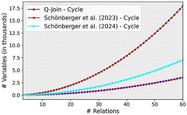
Figure 4. Comparison of the number of mandatory variables in the study by Schönberger et al. (2023a,b) to all variables in our optimization model.

6 Experimental evaluation

In this section, we present the results of a comprehensive experimental evaluation that includes optimizing join order selection on various combinations of query graphs, problem formulations, and classical and quantum optimizers. For each method proposed in this article, we evaluate the technique against five common query graph types: clique, star, chain, cycle, and tree. Each query graph is labeled using the format 'Graph name - number of nodes'. For each graph type and graph size, we sampled 20 query graph instances with random cardinalities and selectivities. The cardinalities are randomly sampled from the range 10 to 50, and selectivity from the interval (0, 1]. The costs are summed over the 20 query graph instances, describing a realistic cumulative error, and scaled with respect to the cost returned from the dynamic programming algorithm with cross products, which is the optimal left-deep plan. This means that the results are compared to the optimal left-deep plans. The code, the exact query graphs, and parameters used for this experimental evaluation are available in the GitHub repository (Uotila, 2025a). Since we have used 20 query graph instances for five different graph types, ranging in size from 3 to 60, and solved them with four different quantum and classical solvers, the total number of optimized problems is in the thousands. We refer to the implementation of our algorithms as Q-Join.

After fixing one of the three proposed methods and a query graph instance, we constructed the corresponding HUBO optimization problem. Then, we submitted the problem for each selected solver. The available solvers include two quantum computing approaches (D-Wave quantum annealer and D-Wave hybrid quantum annealer) and two classical approaches (exact poly solver and Gurobi optimizer). In all cases except the exact poly solver, the HUBO problem needs to be translated into the equivalent QUBO problem.

Our evaluation focuses on solution quality, rather than solver runtime. A direct comparison of execution times is impractical, as system-level latencies heavily influence them. A direct comparison of execution times might be misleading in this scenario because the quantum annealer's microsecond-scale annealing time is only one component of a larger process that includes significant classical overhead from problem embedding and post-processing. The pre- and post-processing latencies include problem encoding, network communication, solver queuing, and interpreting the result. We identify that a meaningful comparison of execution times between classical and quantum systems is still a research question.

Summary of proposed methods. We have proposed three algorithms to solve the join order selection problem with a higher-order unconstrained binary optimization model. Table 1 introduces names for these methods, which are used in this Experimental Evaluation section.

Table 1

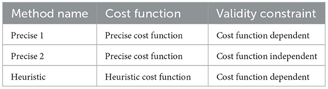
Table 1. Summary of proposed algorithms.

The results should be interpreted as follows. For each case, we have solved the join order selection problem using four different methods: our algorithm in evaluation, dynamic programming without cross products, a greedy algorithm without cross products, and finally, dynamic programming with cross products. Since dynamic programming with cross products produces the optimal left-deep plan, we scale the cumulative cost over 20 different join order optimization problems with this cost. This way, we obtain a metric that enables us to compare these methods without explicitly dealing with cost values. The actual range of costs is arbitrary since the cardinalities and selectivities are randomly sampled. For example, suppose our algorithm has a scaled cost of 1.007. In that case, this means that the cumulative cost of the 20 returned plans from our algorithm is 0.7% larger than the cumulative cost for the optimal plans from dynamic programming with cross products.

6.1 Evaluating Precise 1 formulation

First, we evaluate Precise 1 formulation, which combines a precise cost function and cost-dependent validity constraints. Figure 5 shows the results of optimizing join order selection using D-Wave's exact poly solver, which is part of the Ocean framework. Following the bounds given by Theorem 3, the HUBO model consistently generates a plan that matches the quality of the plan produced by the dynamic programming algorithm without the cross products. We also observe that the returned plans are at most 0.7% larger than the optimal plan from dynamic programming with the cross products.

Figure 5

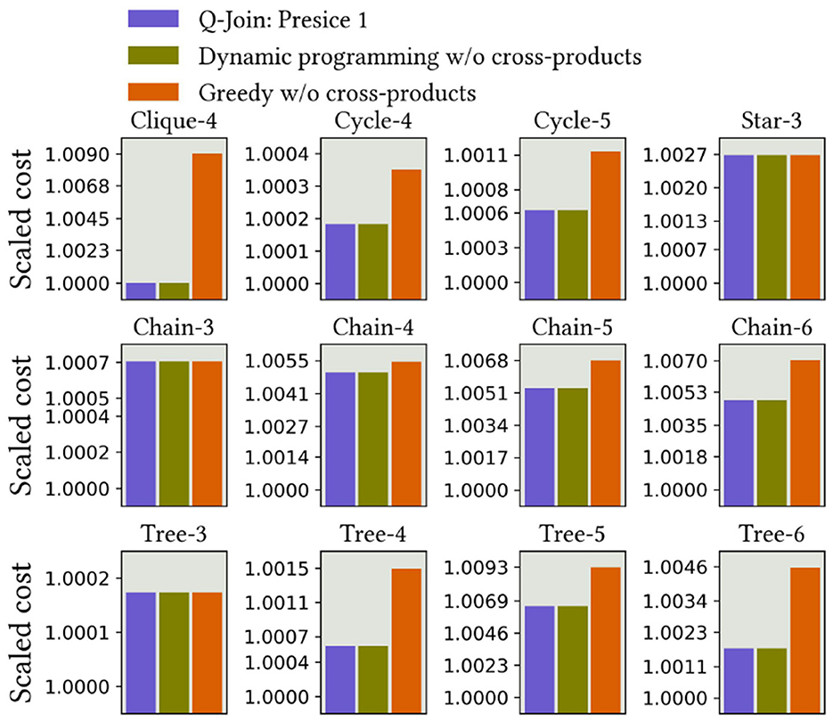
Figure 5. Precise 1 results using D-Wave's exact poly solver. For Clique-3, Cycle-3, Star-4, and Star-5, all three methods achieved optimal cost.

Second, we solved the same HUBO formulations using the classical Gurobi solver. The results are presented in Figure 6. The HUBO-to-QUBO translation does not decrease the algorithm's quality, and the method is able to find the correct plans. The results remain very close to the optimal join tree, consistently matching the quality of the dynamic programming algorithm that does not use cross products.

Figure 6

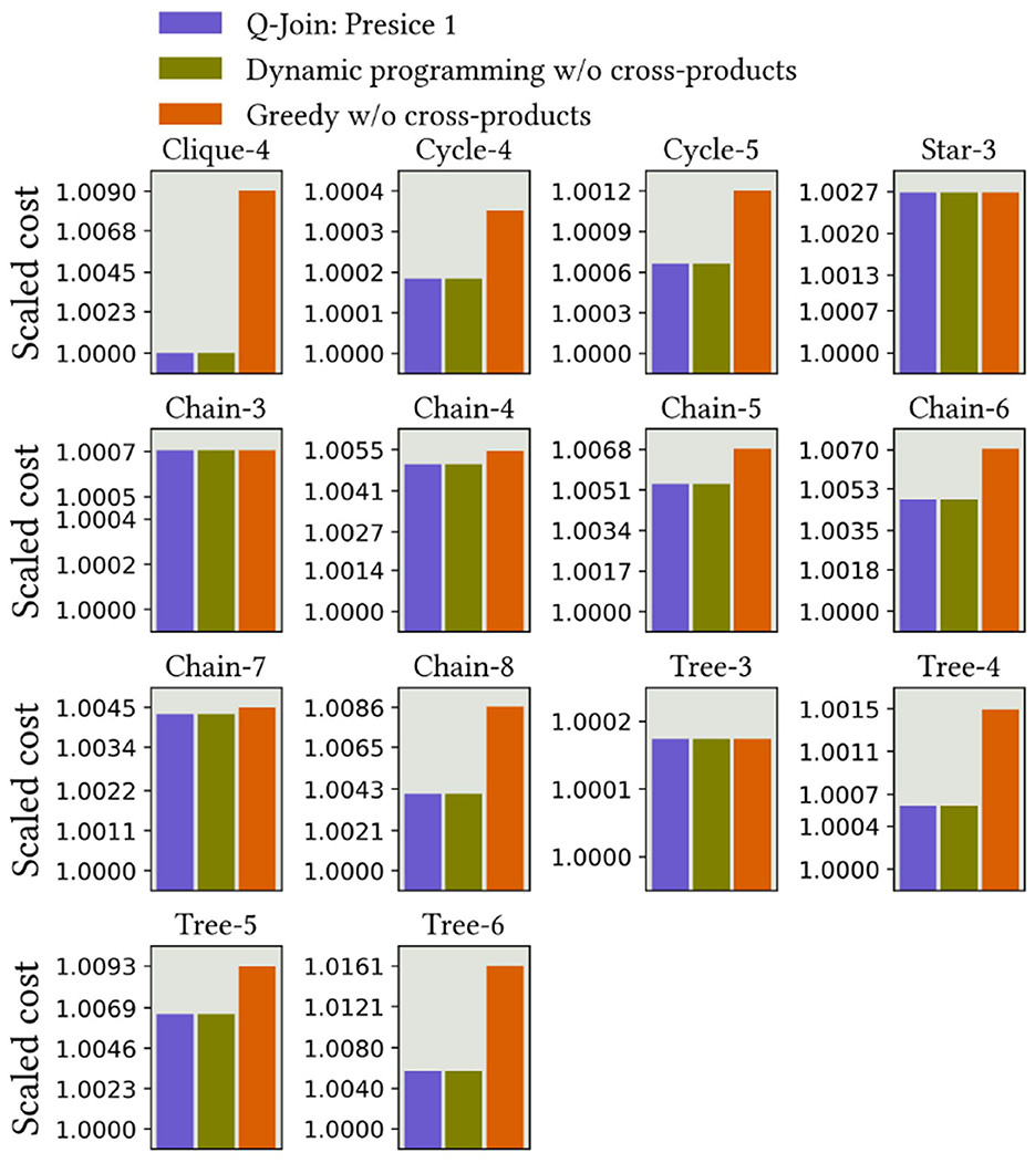
Figure 6. Precise 1 results using Gurobi solver.

Third, we addressed the same problems using D-Wave's Leap Hybrid solver, a cloud-based quantum-classical optimization platform. The results are in Figure 7. In this case, the results are consistently as good as those from the dynamic programming algorithm without the cross products, with some exceptions due to the heuristic nature of the quantum computer: Cycle-6, Chain-7, and Tree-6.

Figure 7

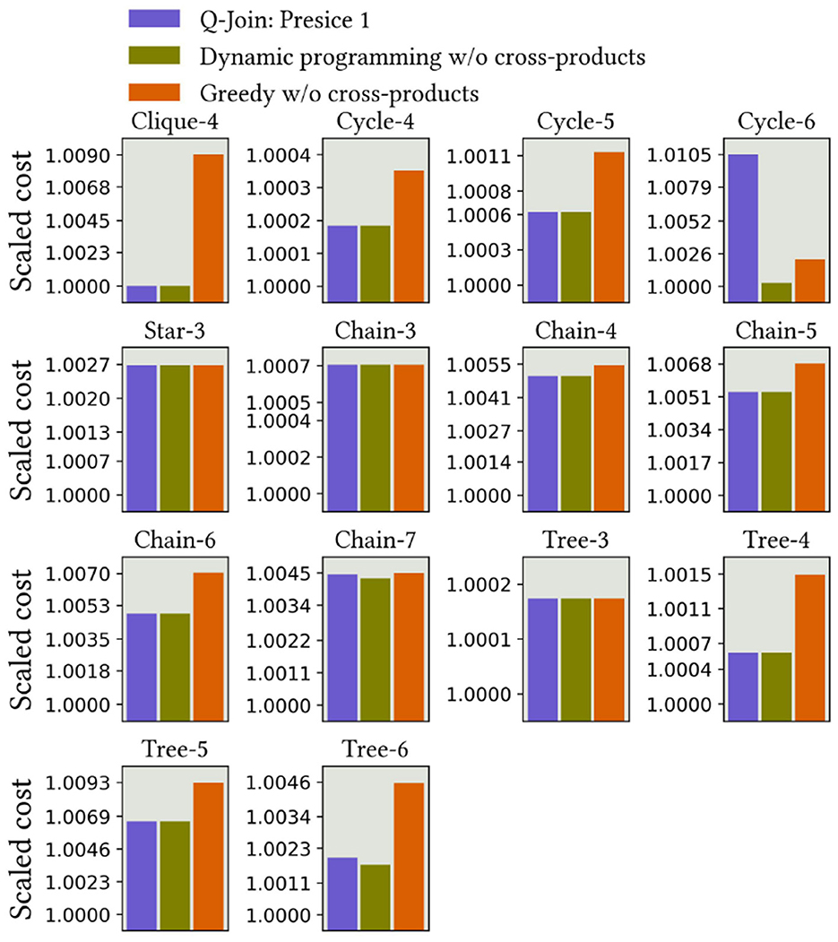
Figure 7. Precise 1 results using D-Wave's Leap Hybrid solver.

Finally, Figure 8 shows the results from D-Wave's quantum annealer, which does not use hybrid features to increase solution quality. This resulted in performance that did not match that of the previous solvers, and this performance decrease had already been identified in the study by Schönberger et al. (2023a). While the quality was not as good as the previous solutions, the valid plans might still be usable, with only a few percent deviation from the global optimum.

Figure 8

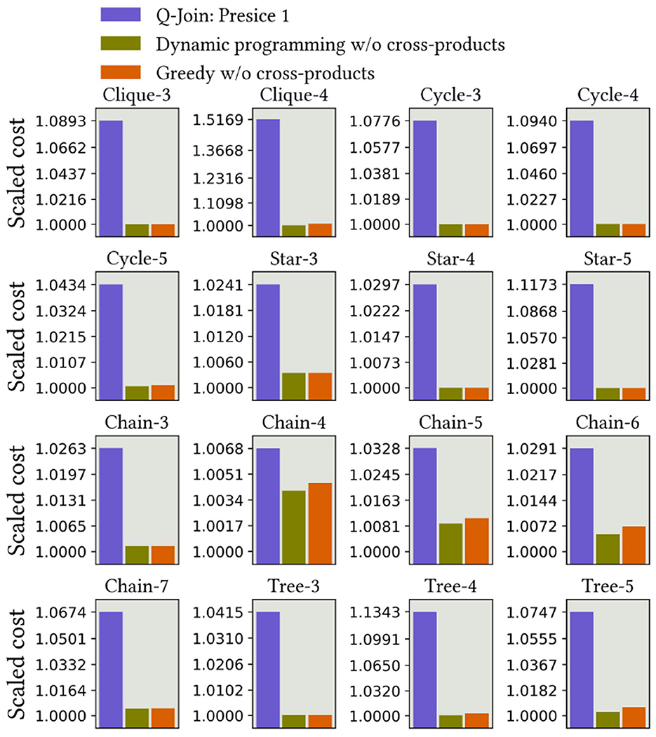
Figure 8. Precise 1 results using D-Wave's quantum annealer without hybrid features.

6.2 Evaluating Precise 2 formulation

The key idea behind the Precise 2 formulation is to tackle larger join order optimization cases, as the validity constraints are more efficient in terms of the number of higher-order terms. We include the exact poly solver results to demonstrate that this formulation encodes precisely the correct plans. For the other solvers, we only show results that optimized larger queries compared to the previous Precise 1 method.

First, the results from the exact poly solver in Figure 9 demonstrate that this algorithm follows the bounds of Theorem 3. In practice, the returned plans are again very close to the optimal plans. We can also see that compared to the Precise 1 method, the different set of validity constraints work equally well.

Figure 9

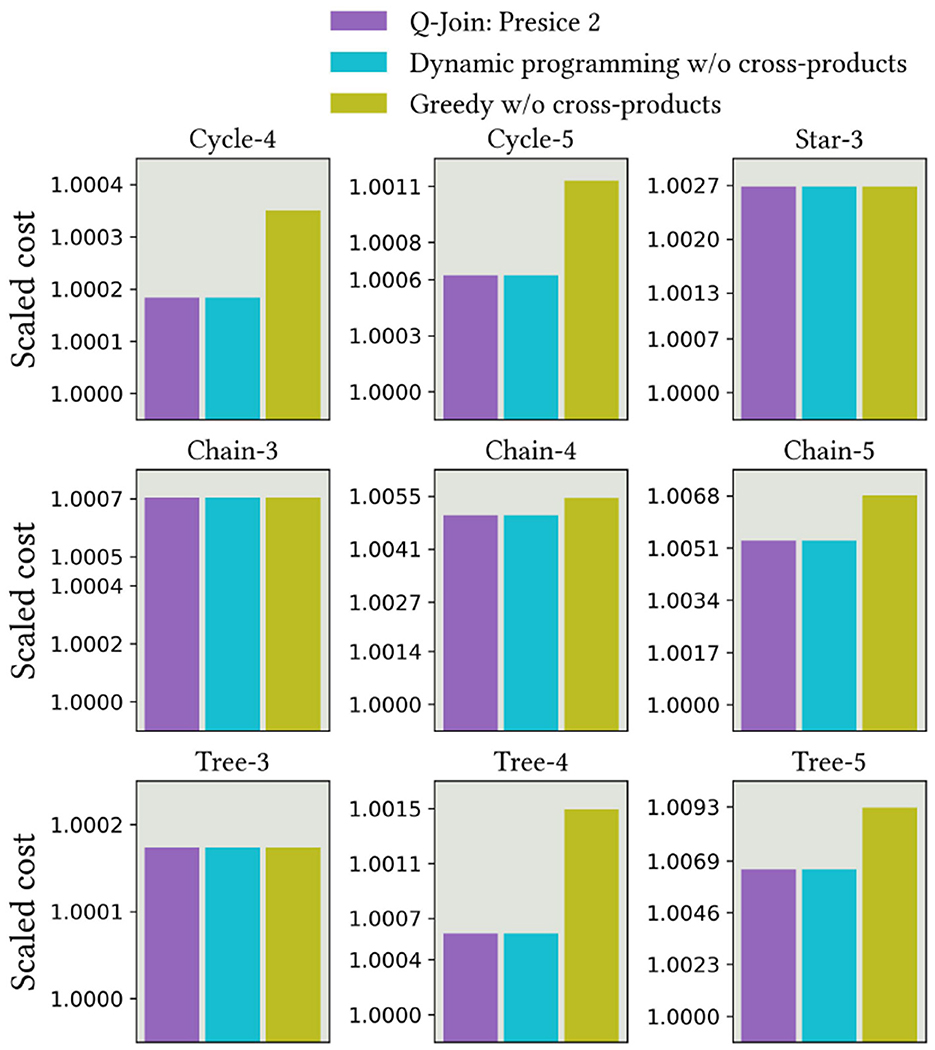
Figure 9. Precise 2 results using D-Wave's exact poly solver.

Second, to evaluate the Gurobi solver, we scaled up the problem sizes significantly from the Precise 1 method. The results are presented in Figure 10. On the other hand, we observed that finding the point that minimizes both cost and validity constraints becomes increasingly challenging as the problem sizes increase.

Figure 10

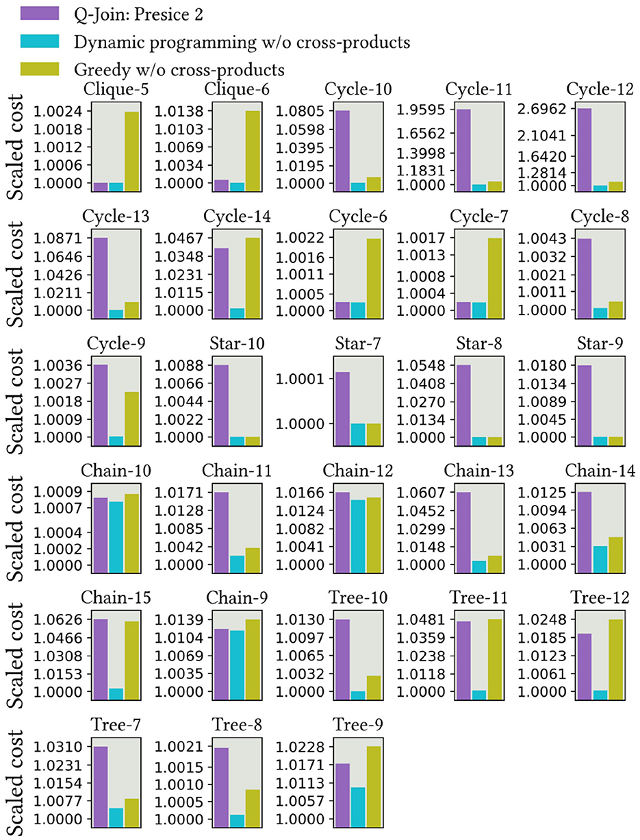
Figure 10. Precise 2 results that were not part of Precise 1 results using Gurobi solver.

Slightly unexpectedly, the hybrid solver did not perform as well as we expected, as shown in Figure 11. The solver does not have tunable hyperparameters, which could be adjusted to obtain better results. Finally, we do not include the results from the D-Wave quantum solver without hybrid features since the solver did not scale beyond the cases that were already presented in Figure 8.

Figure 11

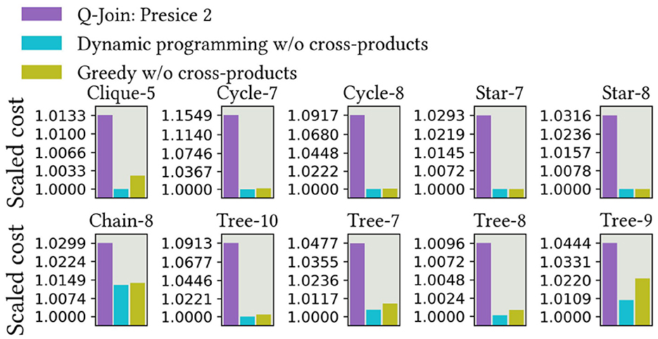
Figure 11. Precise 2 results using D-Wave's Leap Hybrid solver.

6.3 Evaluating heuristic formulation

The key motivation behind the heuristic formulation is to tackle even larger query graphs. Our main goal is to demonstrate that this algorithm reaches acceptable results with superior scalability compared to the previous Precise 1 and 2 formulations. The results also indicate that Theorem 4 is respected in practice. The optimal results are now computed with dynamic programming without cross products. Due to space limitations, we only included the results from the Gurobi solver, which we consider the most demonstrative, and we had unlimited access to it since it runs locally.

The results are presented so that we have computed and scaled the difference between each pair of methods. A value that differs from 0 indicates that the two methods gave different join trees with different costs. Since one of the methods is near-optimal (DP without cross products), it is clear which method produced the suboptimal result. This way, we can compare all three methods simultaneously. In all cases, we observe that the heuristic algorithm respects Theorem 4 in practice, meaning that the formulation produced a plan with a cost equal to the classical greedy algorithm.

Figure 12 shows the results of applying the heuristic method to chain, cycle, and clique query graphs. Scalability for clique graphs in this complex case is modest, and greedy plans are generally far from optimal plans for both our method and the classical greedy algorithm. The results for chain graphs and cycle graphs demonstrate the best scalability. For cycle graphs, our greedy method was able to find better plans than the classical greedy algorithm.

Figure 12

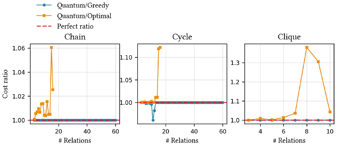
Figure 12. Heuristic results for different query graph topologies using Gurobi solver. Optimal results were solvable up to 16 relations. Considering the results for star and tree graphs, our algorithm and the greedy algorithm without cross products, we consistently obtained the same results.

6.4 Comparison with quantum-inspired digital annealing

We evaluated the method proposed in the study by Schönberger et al. (2023b) using the same workloads and present the results in Figure 13. Their technique is the improved algorithm from the study by Schönberger et al. (2023a). The results demonstrate that our methods perform at the same level as theirs on these workloads. The authors propose a novel readout technique that enhances the results. Since we could not access special quantum-inspired hardware, the digital annealer, we used the Gurobi solver, which returns only a single result by default. Thus, the readout technique was not applicable. In the studied cases, it did not seem to decrease quality.

Figure 13

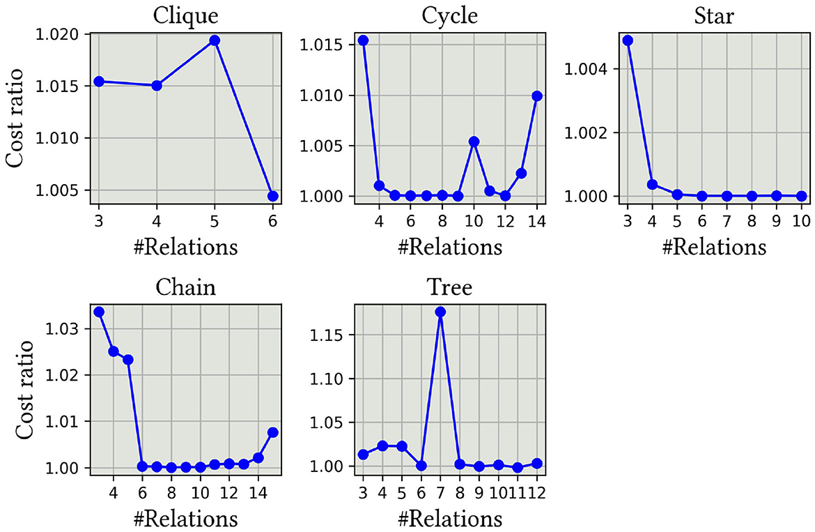
Figure 13. QUBO formulation accuracy on different query graph topologies with QUBO formulation proposed in the study by Schönberger et al. (2023b).

The results demonstrate that their method achieves a comparable accuracy to ours, which is optimal or nearly optimal. We have computed the exact results with dynamic programming using cross products and compared the relative cumulative costs between the methods. Their method also appears to be able to identify beneficial cross products. Due to the higher-order terms in our method, which currently need to be rewritten in quadratic format, their method remains more scalable than ours. On the other hand, our theoretical bounds, query-graph-aware problem formulation, the more straightforward variable definition, and the novel usage of the higher-order model demonstrate specific contributions and improvements over their methods. We are also confident that our model will incorporate features that enable expansion for outer joins, accommodate more complex dependencies between predicates, and allow the usage of other types of cost functions.

7 Discussion

In this study, we developed a novel higher-order binary optimization formulation for optimizing join order selection for left-deep query plans. This is a fundamentally new approach to one of the most studied query optimization problems in the database domain. Our formulation is accompanied by formal guarantees, as proven in Theorems 3 and 4. Our method respects query graphs, which makes it distinct from previous formulations. Although this leaves out cross products, it also simplifies problem formulation for certain query graphs. It paves the way for future methods that rely on information about query graphs. As shown in Figure 4, our method requires a relatively small number of binary variables. Finally, we conducted a comprehensive experimental evaluation that demonstrated the usage of quantum annealers in this task, deepened our understanding of differences between quantum and classical solvers in this real-life problem, and showed that the results in Theorems 3 and 4 are respected in practice.

The starting point for our study has been primarily the previous quantum computing formulations (Schönberger et al., 2023a; Winker et al., 2023a; Schönberger et al., 2023c; Nayak et al., 2024; Franz et al., 2024; Schönberger et al., 2023b; Saxena et al., 2024) for the join order selection problem. Our method's scalability in real-life problems outperforms many previous studies (Schönberger et al., 2023a; Franz et al., 2024; Schönberger et al., 2023c), where the authors have demonstrated their algorithms with 2 to 7 relations. The method proposed in the study by Schönberger et al. (2023b) offers the best scalability and accuracy. However, their algorithm lacks a guarantee of optimality and requires the use of more variables (Figure 4). The comparison to this approach showed accuracy similar to our method in small query graphs. We also note that classical solvers compete with the quantum annealers in this task, even though they run locally on a laptop. This demonstrates that quantum annealers are not scalable enough to solve these types of problems efficiently, and their performance is crucially problem-dependent.

Classical approaches for solving HUBO problems typically rely on approximate methods due to the exponential growth in complexity of these problems. Integer programming can be used to find approximate solutions for HUBO problems, but it suffers from scalability issues and does not always ensure feasibility (Munoz, 2017). Machine learning techniques, including graph neural networks, have been explored for approximating HUBO solutions (Schuetz et al., 2022). However, these approaches often require training data and may struggle to generalize to previously unseen instances. Simulated annealing has been applied as another classical strategy for tackling HUBO problems (Wang et al., 2025). While these classical methods are effective for small- and medium-sized instances, they encounter significant challenges as problem size increases, highlighting the potential usability of quantum-native approaches such as QAOA. In theory, the HUBO formulations in this article can be addressed using the same QAOA-based methods employed in Uotila et al. (2025).

Quantum computing for HUBO problems represents an emerging area in the field of quantum optimization. For example, Campbell and Dahl (2022) explored the use of the Quantum Approximate Optimization Algorithm (QAOA) for higher-order graph coloring problems. Techniques such as bias-field digitized counterdiabatic quantum optimization have been developed to enhance the solution of higher-order binary problems (Romero et al., 2025; Cadavid et al., 2025), and various methods have been proposed for optimizing variational quantum circuits tailored to these challenges (Verchere et al., 2023). Higher-order problems have also served as benchmarks for comparing QAOA and quantum annealing performance (Pelofske et al., 2023; Sachdeva et al., 2024; Pelofske et al., 2024b; Gilbert et al., 2023), as well as for studying the scaling behavior and parameter concentration properties of QAOA (Pelofske et al., 2024a). Initial applications for HUBO formulations include higher-order portfolio optimization (Uotila et al., 2025), the formalization of practical matrix multiplication algorithm search (Uotila, 2024b), and optimization in railway rescheduling (Domino et al., 2022). While HUBO formulations are classically challenging, it remains open whether they offer an actual computational advantage on quantum hardware.

Multiple challenges remain. The biggest challenge in our method is the higher-order terms, whose number grows exponentially in some cases. The current HUBO problem formulations also do not account for bushy trees or cross products, which would further enhance the quality of the solution. We are also limited to inner joins and the simple cost model. The problem of optimizing join order selection also relies on cardinality estimations, which is a separate challenge in query optimization. Finally, there is considerable room for improvement in solving HUBO problems on both classical and quantum hardware. Very few methods can effectively tackle HUBO optimization problems. In this regard, quantum computing appears to be theoretically one of the most promising approaches to optimizing complex HUBOs. In future research, we are excited to explore the universal quantum computing capabilities for solving HUBOs. Unfortunately, the problem sizes studied in this work were still too large for the current universal quantum computers.

Previous methods have been limited to inner joins. Extending our binary variables to model non-inner joins is theoretically straightforward, for instance, by adding a component to indicate the join type (inner or outer). While this modification is simple, the cost function and constraints also need adjustments. Since our cost HUBO is explicitly based on the recursive join order cost function, encoding predicate dependencies is also feasible. Our HUBO formulations can be further approximated with other heuristics to make them feasible for solving a larger set of complex query graphs. Exploring these extensions offers promising directions for future research in join order optimization with quantum computing.

8 Conclusion

In this study, we have developed three novel graph-aware higher-order binary optimization models to solve the join order selection problem in relational databases. The HUBO problems can be divided into cost functions and validity constraints. We presented two new binary optimization formulations for the cost function and proved that one encodes the same join trees as the dynamic programming algorithm without cross products. The other finds plans that are at least as good as those returned by the greedy algorithm without cross products. Finally, we presented a comprehensive experimental evaluation of these algorithms on various quantum and classical solvers. The experimental evaluation demonstrated the practical usability of these HUBO formulations and the fact that we respect the proven bounds in practice. While classical solvers remained competitive, these types of binary optimization models will serve as the essential element for future quantum optimization platforms.

Data availability statement

The datasets presented in this study can be found in online repositories. The names of the repository/repositories and accession number(s) can be found in the article/supplementary material.

Author contributions

VU: Writing – original draft, Software, Writing – review & editing, Data curation, Conceptualization, Investigation, Formal analysis, Visualization, Methodology.

Funding

The author(s) declare that financial support was received for the research and/or publication of this article. Open access funded by Helsinki University Library.

Conflict of interest

The author declares that the research was conducted in the absence of any commercial or financial relationships that could be construed as a potential conflict of interest.

Generative AI statement

The author(s) declare that Gen AI was used in the creation of this manuscript. Generative AI was used to improve the quality of language, code and visualizations.

Any alternative text (alt text) provided alongside figures in this article has been generated by Frontiers with the support of artificial intelligence and reasonable efforts have been made to ensure accuracy, including review by the authors wherever possible. If you identify any issues, please contact us.

Publisher's note

All claims expressed in this article are solely those of the authors and do not necessarily represent those of their affiliated organizations, or those of the publisher, the editors and the reviewers. Any product that may be evaluated in this article, or claim that may be made by its manufacturer, is not guaranteed or endorsed by the publisher.

References

Abbas, A., Ambainis, A., Augustino, B., Baertschi, A., Buhrman, H., Coffrin, C. J., et al. (2024). Quantum Optimization: Potential, Challenges, and the Path Forward. Washington, DC: US Department of Energy.

PubMed Abstract | Google Scholar

Aharonov, D., van Dam, W., Kempe, J., Landau, Z., Lloyd, S., Regev, O., et al. (2004). Adiabatic quantum computation is equivalent to standard quantum computation. arXiv [preprint]. arXiv:quant-ph/0405098v2. doi: 10.48550/arXiv.quant-ph/0405098v2

PubMed Abstract | Crossref Full Text | Google Scholar

Albash, T., and Lidar, D. A. (2018). Adiabatic quantum computation. Rev. Mod. Phys. 90, 015002. doi: 10.1103/RevModPhys.90.015002

Crossref Full Text | Google Scholar

Apolloni, B., Carvalho, C., and de Falco, D. (1989). Quantum stochastic optimization. Stoch. Processes Appl. 33, 233–244. doi: 10.1016/0304-4149(89)90040-9

Crossref Full Text | Google Scholar

Aramon, M., Rosenberg, G., Valiante, E., Miyazawa, T., Tamura, H., Katzgraber, H. G., et al. (2019). Physics-inspired optimization for quadratic unconstrained problems using a digital annealer. Front. Phys. 7:48. doi: 10.3389/fphy.2019.00048

Crossref Full Text | Google Scholar

Arute, F., Arya, K., Babbush, R., Bacon, D., Bardin, J. C., Barends, R., et al. (2019). Quantum supremacy using a programmable superconducting processor. Nature 574, 505–510. doi: 10.1038/s41586-019-1666-5

PubMed Abstract | Crossref Full Text | Google Scholar

Bittner, T., and Groppe, S. (2020). “Avoiding blocking by scheduling transactions using quantum annealing,” in Proceedings of the 24th Symposium on International Database Engineering & Applications, IDEAS '20 (New York, NY: Association for Computing Machinery), 1–10. doi: 10.1145/3410566.3410593

Crossref Full Text | Google Scholar

Boros, E., and Hammer, P. L. (2002). Pseudo-boolean optimization. Discrete Appl. Math. 123, 155–225. doi: 10.1016/S0166-218X(01)00341-9

Crossref Full Text | Google Scholar

Cadavid, A. G., Dalal, A., Simen, A., Solano, E., and Hegade, N. N. (2025). Bias-field digitized counterdiabatic quantum optimization. Phys. Rev. Res. 7:L022010. doi: 10.1103/PhysRevResearch.7.L022010

Crossref Full Text | Google Scholar

Çalikyilmaz, U., Groppe, S., Groppe, J., Winker, T., Prestel, S., Shagieva, F., et al. (2023). Opportunities for quantum acceleration of databases: optimization of queries and transaction schedules. VLDB 16, 2344–2353. doi: 10.14778/3598581.3598603

Crossref Full Text | Google Scholar

Campbell, C., and Dahl, E. (2022). “Qaoa of the highest order,” in 2022 IEEE 19th International Conference on Software Architecture Companion (ICSA-C) (Honolulu, HI: IEEE), 141–146. doi: 10.1109/ICSA-C54293.2022.00035

Crossref Full Text | Google Scholar

Cluet, S., and Moerkotte, G. (1995). “On the complexity of generating optimal left-deep processing trees with cross products,” in Database Theory – ICDT '95, eds. G. Gottlob, and M. Y. Vardi (Berlin, Heidelberg: Springer Berlin Heidelberg), 54–67. doi: 10.1007/3-540-58907-4_6

PubMed Abstract | Crossref Full Text | Google Scholar

Denchev, V. S., Boixo, S., Isakov, S. V., Ding, N., Babbush, R., Smelyanskiy, V., et al. (2016). What is the computational value of finite-range tunneling? Phys. Rev. X 6:031015. doi: 10.1103/PhysRevX.6.031015

Crossref Full Text | Google Scholar

Domino, K., Kundu, A., Salehi, Ö., and Krawiec, K. (2022). Quadratic and higher-order unconstrained binary optimization of railway rescheduling for quantum computing. Quantum Inf. Process. 21:337. doi: 10.1007/s11128-022-03670-y

Crossref Full Text | Google Scholar

D-Wave Quantum Inc. (2024). Non-Quadratic (Higher-Degree) Polynomials. Available online at: https://docs.dwavequantum.com/en/latest/quantum_research/reformulating.html#non-quadratic-higher-degree-polynomials (Accessed February 01, 2024).

Google Scholar

D-Wave Quantum Inc. (2025). What is Quantum Annealing? Available online at: https://docs.dwavequantum.com/en/latest/quantum_research/quantum_annealing_intro.html (Accessed June 16, 2025).

Google Scholar

D-Wave Systems Inc. (2024). Dimod.Generators.Combinations. Available online at: https://docs.ocean.dwavesys.com/en/stable/docs_dimod/reference/generated/dimod.generators.combinations.html (Accessed: October 12, 2024).

Google Scholar

Farhi, E., Goldstone, J., Gutmann, S., and Sipser, M. (2000). Quantum computation by adiabatic evolution. arXiv [preprint]. arXiv:quant-ph/0001106. doi: 10.48550/arXiv.quant-ph/0001106

Crossref Full Text | Google Scholar

Franz, M., Winker, T., Groppe, S., and Mauerer, W. (2024). Hype or heuristic? quantum reinforcement learning for join order optimisation. arXiv [preprint]. arXiv:2405.07770. doi: 10.48550/arXiv.2405.07770

Crossref Full Text | Google Scholar

Fritsch, K., and Scherzinger, S. (2023). Solving hard variants of database schema matching on quantum computers. Proc. VLDB Endowment 16, 3990–3993. doi: 10.14778/3611540.3611603

Crossref Full Text | Google Scholar

Gilbert, V., Rodriguez, J., Louise, S., and Sirdey, R. (2023). “Solving higher order binary optimization problems on nisq devices: experiments and limitations,” in Lecture Notes in Computer Science, volume LNCS-10477 of Computational Science – ICCS 2023, page 224–232, Prague, Czech Republic, eds. J. Mikyška, C. D. Mulatier, M. Paszynski, V. V. Krzhizhanovskaya, J. J. Dongarra, and P. M. A. Sloot (Cham: Springer Nature Switzerland). doi: 10.1007/978-3-031-36030-5_18

Crossref Full Text | Google Scholar

Gill, S. S., Kumar, A., Singh, H., Singh, M., Kaur, K., Usman, M., et al. (2022). Quantum computing: A taxonomy, systematic review and future directions. Softw. Pract. Exp. 52, 66–114. doi: 10.1002/spe.3039

PubMed Abstract | Crossref Full Text | Google Scholar

Grimm, R., Weidemüller, M., and Ovchinnikov, Y. B. (2000). “Optical dipole traps for neutral atoms,” in Advances In Atomic, Molecular, and Optical Physics, Vol. 42 (New York, NY: Academic Press), 95–170. doi: 10.1016/S1049-250X(08)60186-X

Crossref Full Text | Google Scholar

Grover, L. K. (1996). “A fast quantum mechanical algorithm for database search,” in Proceedings of the Twenty-Eighth Annual ACM Symposium on Theory of Computing, STOC '96 (New York, NY: Association for Computing Machinery), 212–219. doi: 10.1145/237814.237866

Crossref Full Text | Google Scholar

Gruenwald, L., Winker, T., Çalikyilmaz, U., Groppe, J., and Groppe, S. (2023). “Index tuning with machine learning on quantum computers for large-scale database applications,” in Joint Workshops at 49th International Conference on Very Large Data Bases (VLDBW'23) — International Workshop on Quantum Data Science and Management (QDSM'23) (Vancouver, BC).

Google Scholar

Harrow, A., and Montanaro, A. (2017). Quantum computational supremacy. Nature 549, 203–209. doi: 10.1038/nature23458

PubMed Abstract | Crossref Full Text | Google Scholar

Ibaraki, T., and Kameda, T. (1984). On the optimal nesting order for computing n-relational joins. ACM Trans. Database Syst. 9, 482–502. doi: 10.1145/1270.1498

Crossref Full Text | Google Scholar

Kadowaki, T., and Nishimori, H. (1998). Quantum annealing in the transverse ising model. Phys. Rev. E 58, 5355–5363. doi: 10.1103/PhysRevE.58.5355

Crossref Full Text | Google Scholar

Kim, Y., Eddins, A., Anand, S., Wei, K. X., van den Berg, E., Rosenblatt, S., et al. (2023). Evidence for the utility of quantum computing before fault tolerance. Nature 618, 500–505. doi: 10.1038/s41586-023-06096-3

PubMed Abstract | Crossref Full Text | Google Scholar

King, A. D., Nocera, A., Rams, M. M., Dziarmaga, J., Wiersema, R., Bernoudy, W., et al. (2024). Computational supremacy in quantum simulation. arXiv [preprint]. arXiv:2403.00910 [cond-mat, physics:quant-ph]. doi: 10.48550/arXiv.2403.00910

Crossref Full Text | Google Scholar

Kirkpatrick, S., Gelatt, C. D., and Vecchi, M. P. (1983). Optimization by simulated annealing. Science 220, 671–680. doi: 10.1126/science.220.4598.671

PubMed Abstract | Crossref Full Text | Google Scholar

Kittelmann, F., Sulimov, P., and Stockinger, K. (2024). “Qardest: using quantum machine learning for cardinality estimation of join queries,” in Workshop on Quantum Computing and Quantum-Inspired Technology for Data-Intensive Systems and Applications, Q-Data 2024, Santiago, Chile, June 9-15, 2024 (New York, NY: ACM), I. Sabek, I. Trummer, and S. Prestel doi: 10.1145/3665225.3665444

Crossref Full Text | Google Scholar

Knill, E., Laflamme, R., and Milburn, G. J. (2001). A scheme for efficient quantum computation with linear optics. Nature 409, 46–52. doi: 10.1038/35051009

PubMed Abstract | Crossref Full Text | Google Scholar

Leis, V., Gubichev, A., Mirchev, A., Boncz, P., Kemper, A., Neumann, T., et al. (2015). How good are query optimizers, really? Proc. VLDB Endow. 9, 204–215. doi: 10.14778/2850583.2850594

Crossref Full Text | Google Scholar

Liu, H., Kumar, A., Spedalieri, F., and Sabek, I. (2025). “Hybrid quantum-classical optimization for bushy join trees,” in Proceedings of the 2nd Workshop on Quantum Computing and Quantum-Inspired Technology for Data-Intensive Systems and Applications, Q-Data '25 (New York, NY: Association for Computing Machinery), 20–24. doi: 10.1145/3736393.3736695

Crossref Full Text | Google Scholar

Lucas, A. (2014). Ising formulations of many np problems. Front. Phys. 2:5. doi: 10.3389/fphy.2014.00005

Crossref Full Text | Google Scholar

Madsen, L. S., Laudenbach, F., Askarani, M. F., Rortais, F., Vincent, T., Bulmer, J. F. F., et al. (2022). Quantum computational advantage with a programmable photonic processor. Nature 606, 75–81. doi: 10.1038/s41586-022-04725-x

PubMed Abstract | Crossref Full Text | Google Scholar

Mc Keever, C., and Lubasch, M. (2024). Towards adiabatic quantum computing using compressed quantum circuits. PRX Quantum 5:020362. doi: 10.1103/PRXQuantum.5.020362

Crossref Full Text | Google Scholar

Moerkotte, G., and Neumann, T. (2006). “Analysis of two existing and one new dynamic programming algorithm for the generation of optimal bushy join trees without cross products,” in Proceedings of the 32nd International Conference on Very Large Data Bases, VLDB '06 (Seoul: VLDB Endowment), 930–941.

Google Scholar

Moerkotte, G., and Neumann, T. (2008). “Dynamic programming strikes back,” in Proceedings of the 2008 ACM SIGMOD International Conference on Management of Data (Vancouver, BC: ACM), 539–552. doi: 10.1145/1376616.1376672

Crossref Full Text | Google Scholar

Munoz, G. (2017). Integer Programming Techniques for Polynomial Optimization. New York, NY: Columbia University.

Google Scholar

Nayak, N., Prisacaru, A., Çalıkyılmaz, U., Groppe, J., and Groppe, S. (2025). “Quantum-enhanced transaction scheduling with reduced complexity via solving qubo iteratively using a locking mechanism,” in Proceedings of the 2nd Workshop on Quantum Computing and Quantum-Inspired Technology for Data-Intensive Systems and Applications, Q-Data '25 (New York, NY: Association for Computing Machinery), 26–35. doi: 10.1145/3736393.3736701

Crossref Full Text | Google Scholar

Nayak, N., Winker, T., Çalikyilmaz, U., Groppe, S., and Groppe, J. (2024). Quantum join ordering by splitting the search space of qubo problems. Datenbank-Spektrum 24, 21–32. doi: 10.1007/s13222-024-00468-3

Crossref Full Text | Google Scholar

Neumann, P., Mizuochi, N., Rempp, F., Hemmer, P., Watanabe, H., Yamasaki, S., et al. (2008). Multipartite entanglement among single spins in diamond. Science 320, 1326–1329. doi: 10.1126/science.1157233

PubMed Abstract | Crossref Full Text | Google Scholar

Neumann, T., and Gubichev, A. (2014). Query Optimization. Technische Universität München; Chair for Database Systems. Available online at: https://db.in.tum.de/teaching/ws1415/queryopt/?lang=en (Accessed September 23, 2025).

Google Scholar

Neumann, T., and Radke, B. (2018). “Adaptive optimization of very large join queries,” in Proceedings of the 2018 International Conference on Management of Data, SIGMOD '18 (New York, NY: Association for Computing Machinery), 677–692. doi: 10.1145/3183713.3183733

Crossref Full Text | Google Scholar

Nielsen, M. A., and Chuang, I. L. (2010). Quantum Computation and Quantum Information: 10th Anniversary Edition. Cambridge: Cambridge University Press.

Google Scholar

Ono, K., and Lohman, G. M. (1990). “Measuring the complexity of join enumeration in query optimization,” in Proceedings of the 16th International Conference on Very Large Data Bases, VLDB '90 (San Francisco, CA: Morgan Kaufmann Publishers Inc), 314–325.

Google Scholar

Paul, W. (1990). Electromagnetic traps for charged and neutral particles. Rev. Mod. Phys. 62:531. doi: 10.1103/RevModPhys.62.531

Crossref Full Text | Google Scholar

Pelofske, E., Bärtschi, A., Cincio, L., Golden, J., and Eidenbenz, S. (2024a). Scaling whole-chip qaoa for higher-order ising spin glass models on heavy-hex graphs. NPJ Quantum Inf. 10, 1–18. doi: 10.1038/s41534-024-00906-w

Crossref Full Text | Google Scholar

Pelofske, E., Bärtschi, A., and Eidenbenz, S. (2023). “Quantum annealing vs. qaoa: 127 qubit higher-order ising problems on NISQ computers,” in High Performance Computing: 38th International Conference, ISC High Performance 2023, Hamburg, Germany, May 21–25, 2023, Proceedings (Berlin, Heidelberg: Springer-Verlag), 240–258. doi: 10.1007/978-3-031-32041-5_13

Crossref Full Text | Google Scholar

Pelofske, E., Bärtschi, A., and Eidenbenz, S. (2024b). Short-depth qaoa circuits and quantum annealing on higher-order ising models. npj Quantum Inf. 10, 1–19. doi: 10.1038/s41534-024-00825-w

Crossref Full Text | Google Scholar

Romero, S. V., Visuri, A.-M., Cadavid, A. G., Simen, A., Solano, E., Hegade, N. N., et al. (2025). Bias-field digitized counterdiabatic quantum algorithm for higher-order binary optimization. Commun. Phys. 8:348. doi: 10.1038/s42005-025-02270-3

Crossref Full Text | Google Scholar

Sachdeva, N., Hartnett, G. S., Maity, S., Marsh, S., Wang, Y., Winick, A., et al. (2024). Quantum optimization using a 127-qubit gate-model ibm quantum computer can outperform quantum annealers for nontrivial binary optimization problems. arXiv [preprint]. arXiv:2406.01743. doi: 10.48550/arXiv.2406.01743

Crossref Full Text | Google Scholar

Saxena, P., Sabek, I., and Spedalieri, F. M. (2024). “Constrained quadratic model for optimizing join orders,” in Workshop on Quantum Computing and Quantum-Inspired Technology for Data-Intensive Systems and Applications, Q-Data 2024, Santiago, Chile, June 9-15, 2024, eds. I. Sabek, I. Trummer, and S. Prestel (New York, NT: ACM). doi: 10.1145/3665225.3665447

Crossref Full Text | Google Scholar

Schönberger, M. (2022). “Applicability of quantum computing on database query optimization,” in Proceedings of the 2022 International Conference on Management of Data (Philadelphia, PA: ACM), 2512–2514. doi: 10.1145/3514221.3520257

PubMed Abstract | Crossref Full Text | Google Scholar

Schönberger, M., Scherzinger, S., and Mauerer, W. (2023a). “Ready to leap (by co-design)? join order optimisation on quantum hardware,” in Proceedings of the ACM on Management of Data (New York, NY: Association for Computing Machinery). doi: 10.1145/3588946

Crossref Full Text | Google Scholar

Schönberger, M., Trummer, I., and Mauerer, W. (2023b). Quantum-inspired digital annealing for join ordering. Proc. VLDB Endow. 17, 511–524. doi: 10.14778/3632093.3632112

Crossref Full Text | Google Scholar

Schönberger, M., Trummer, I., and Mauerer, W. (2023c). “Quantum optimisation of general join trees,” in Joint Workshops at 49th International Conference on Very Large Data Bases (VLDBW'23) — International Workshop on Quantum Data Science and Management (QDSM'23) (Vancouver, BC).

Google Scholar

Schuetz, M. J., Brubaker, J. K., and Katzgraber, H. G. (2022). Combinatorial optimization with physics-inspired graph neural networks. Nat. Mach. Intell. 4, 367–377. doi: 10.1038/s42256-022-00468-6

Crossref Full Text | Google Scholar

Selinger, P. G., Astrahan, M. M., Chamberlin, D. D., Lorie, R. A., and Price, T. G. (1979). “Access path selection in a relational database management system,” in Proceedings of the 1979 ACM SIGMOD International Conference on Management of Data, SIGMOD '79 (New York, NY: Association for Computing Machinery), 23–34. doi: 10.1145/582095.582099

Crossref Full Text | Google Scholar

Shor, P. (1994). “Algorithms for quantum computation: discrete logarithms and factoring,” in Proceedings 35th Annual Symposium on Foundations of Computer Science (Santa Fe, NM: IEEE), 124–134. doi: 10.1109/SFCS.1994.365700

Crossref Full Text | Google Scholar

Steinbrunn, M., Moerkotte, G., and Kemper, A. (1997). Heuristic and randomized optimization for the join ordering problem. VLDB J. 6, 191–208. doi: 10.1007/s007780050040

Crossref Full Text | Google Scholar

Székely, L. A., and Wang, H. (2005). On subtrees of trees. Adv. Appl. Math. 34, 138–155. doi: 10.1016/j.aam.2004.07.002

Crossref Full Text | Google Scholar

Trummer, I. (2025). “Leveraging quantum computing for optimal data allocation in distributed systems,” in Proceedings of the 2nd Workshop on Quantum Computing and Quantum-Inspired Technology for Data-Intensive Systems and Applications, Q-Data '25 (New York, NY: Association for Computing Machinery), 10–17. doi: 10.1145/3736393.3736692

Crossref Full Text | Google Scholar

Trummer, I., and Koch, C. (2016). Multiple query optimization on the d-wave 2x adiabatic quantum computer. Proc. VLDB Endow. 9, 648–659. doi: 10.14778/2947618.2947621

Crossref Full Text | Google Scholar

Trummer, I., and Koch, C. (2017). “Solving the join ordering problem via mixed integer linear programming,” in Proceedings of the 2017 ACM International Conference on Management of Data, SIGMOD '17 (New York, NY: Association for Computing Machinery), 1025–1040. doi: 10.1145/3035918.3064039

Crossref Full Text | Google Scholar

Trummer, I., and Venturelli, D. (2024). “Leveraging quantum computing for database index selection,” in Workshop on Quantum Computing and Quantum-Inspired Technology for Data-Intensive Systems and Applications, Q-Data 2024, Santiago, Chile, June 9-15, 2024, eds. I. Sabek, I. Trummer, and S. Prestel (New York, NY: ACM). doi: 10.1145/3665225.3665445

Crossref Full Text | Google Scholar

Uotila, V. (2022). “Synergy between quantum computers and databases,” in of the VLDB 2022 PhD Workshop co-located with the 48th International Conference on Very Large Databases (VLDB 2022), 3186 (Sydney), 4.

PubMed Abstract | Google Scholar

Uotila, V. (2024a). “Quantum natural language processing application for estimating SQL query metrics,” in 2024 IEEE International Conference on Quantum Computing and Engineering (QCE), Vol. 2 (Montreal, QC: IEEE), 392–393. doi: 10.1109/QCE60285.2024.10321

Crossref Full Text | Google Scholar

Uotila, V. (2024b). “Tensor decompositions and adiabatic quantum computing for discovering practical matrix multiplication algorithms,” in 2024 IEEE International Conference on Quantum Computing and Engineering (QCE), Vol. 01 (Montreal, QC: IEEE), 390–401. doi: 10.1109/QCE60285.2024.00053

Crossref Full Text | Google Scholar

Uotila, V. (2025a). Q-join Github Repository. Available online at: https://github.com/valterUo/Q-Join (Accessed June 16, 2025).

Google Scholar

Uotila, V. (2025b). “Sql2circuits: estimating cardinalities, execution times, and costs for sql queries with quantum natural language processing,” in IEEE International Conference on Quantum Computing and Engineering (QCE) (Albuquerque).

Google Scholar

Uotila, V., Julia, R., and Zhao, B. (2025). “Higher-order portfolio optimization with quantum approximate optimization algorithm,” in 2025 IEEE International Conference on Quantum Computing and Engineering (QCE) (Albuquerque: IEEE).

Google Scholar

Uotila, V., and Lu, J. (2023). “Quantum annealing method for dynamic virtual machine and task allocation in cloud infrastructures from sustainability perspective,” in 2023 IEEE 39th International Conference on Data Engineering Workshops (ICDEW) (Anaheim, CA: IEEE), 105–110. doi: 10.1109/ICDEW58674.2023.00023

Crossref Full Text | Google Scholar

Verchere, Z., Elloumi, S., and Simonetto, A. (2023). “Optimizing variational circuits for higher-order binary optimization,” in 2023 IEEE International Conference on Quantum Computing and Engineering (QCE) (Los Alamitos, CA: IEEE Computer Society), 19–25. doi: 10.1109/QCE57702.2023.00011

PubMed Abstract | Crossref Full Text | Google Scholar

Vogrin, M., Vogrin, R., Groppe, S., and Groppe, J. (2024). “Supervised learning on relational databases with quantum graph neural networks,” in QDSM@VLDB (Guangzhou)

Google Scholar

Wang, B.-Y., Cui, X., Zeng, Q., Zhan, Y., Yung, M.-H., Shi, Y., et al. (2025). Speedup of high-order unconstrained binary optimization using quantum z 2 lattice gauge theory. Commun. Phys. 8:150. doi: 10.1038/s42005-025-02072-7

Crossref Full Text | Google Scholar

Wendin, G. (2017). Quantum information processing with superconducting circuits: a review. Rep. Prog. Phys. 80:106001. doi: 10.1088/1361-6633/aa7e1a

PubMed Abstract | Crossref Full Text | Google Scholar

Willsch, D., Willsch, M., Gonzalez Calaza, C. D., Jin, F., De Raedt, H., Svensson, M., et al. (2022). Benchmarking advantage and d-wave 2000q quantum annealers with exact cover problems. Quantum Inf Process. 21:141. doi: 10.1007/s11128-022-03476-y

Crossref Full Text | Google Scholar

Winker, T., Çalikyilmaz, U., Gruenwald, L., and Groppe, S. (2023a). “Quantum machine learning for join order optimization using variational quantum circuits in Proceedings of the International Workshop on Big Data in Emergent Distributed Environments, BiDEDE '23 (New York, NY: Association for Computing Machinery), 1–7. doi: 10.1145/3579142.3594299

Crossref Full Text | Google Scholar

Winker, T., Groppe, S., Uotila, V., Yan, Z., Lu, J., Franz, M., et al. (2023b). “Quantum machine learning: foundation, new techniques, and opportunities for database research,” in Companion of the 2023 International Conference on Management of Data, SIGMOD '23 (New York, NY: Association for Computing Machinery), 45–52. doi: 10.1145/3555041.3589404

Crossref Full Text | Google Scholar

Zhong, H.-S., Wang, H., Deng, Y.-H., Chen, M.-C., Peng, L.-C., Luo, Y.-H., et al. (2020). Quantum computational advantage using photons. Science 370, 1460–1463. doi: 10.1126/science.abe8770

PubMed Abstract | Crossref Full Text | Google Scholar

Zhu, Q., Cao, S., Chen, F., Chen, M.-C., Chen, X., Chung, T.-H., et al. (2021). Quantum computational advantage via 60-qubit 24-cycle random circuit sampling. arXiv [preprint]. arXiv:2109.03494. doi: 10.48550/arXiv:2109.03494

PubMed Abstract | Crossref Full Text | Google Scholar