Hydrological evaluation of gridded climate datasets in a texas urban watershed using soil and water assessment tool and artificial neural network

1 Introduction

Precipitation is a critical input variable in hydrological modeling. In the past, records from rain gauges have been the primary data sources used to drive watershed level rainfall-runoff models (Beven, 2011) and are often recognized as the most accurate surface precipitation measurement (Stampoulis and Anagnostou, 2012). However, some apparent limitations exist when gauge rainfall data is applied. Most notably, the rain gauge data are point measurements that may have a poor representation of precipitation across a watershed. Worqlul et al. (2014) pointed out that capturing the spatial variation of precipitation in a moderate-sized watershed can be difficult unless a large number of rain gauges is available. In addition, precipitation records from rain gauges are often incomplete both spatially and temporarily (Fuka et al., 2014), especially in remote regions where maintaining a rain gauge network can be challenging and expensive.

In recent decades, alternative precipitation datasets using different measurement approaches have become available. In particular, the availability of satellite rainfall products (SRPs) has vastly improved in the past few years, providing new opportunities for hydrologists to obtain efficient precipitation data in remote regions where ground-based rain gauges are sparse (Worqlul et al., 2014). The Tropical Rainfall Measuring Mission (TRMM) is one of the freely available SRPs. It was designed by NASA and the Japan Aerospace Exploration Agency (JAXA) to monitor and study tropical rainfall (Adler et al., 2003). The TRMM 3B42 product contains a merged microwave/infrared (IR) precipitation estimate band with a 3-h temporal resolution and a 0.25-degree spatial resolution. The TRMM 3B43 dataset is gauge-adjusted and covers the global latitude belt from 50°S to 50°N (Li et al., 2018). Recent studies have evaluated the performance of TRMM products in different regions of the world. Ochoa et al. (2014) compared TRMM data with an interpolated gauge dataset in the Pacific–Andean region in western South America. They concluded that TRMM could capture the seasonal features of precipitation but suggested that TRMM systematically overestimated precipitation in some parts of the study area. Stampoulis and Anagnostou (2012) compared TRMM 3B42 version 6 data against a network of rain gauges over continental Europe, and the authors came to a similar conclusion that TRMM generally overestimated rainfall. Worqlul et al. (2014) compared TRMM 3B42 dataset with two other gridded rainfall products, Multi-Sensor Precipitation Estimate–Geostationary (MPEG) and Climate Forecast System Reanalysis (CFSR), in the Lake Tana Basin in Ethiopia. Their analysis found that MPEG and CFSR have a lower root mean square error (RMSE) with ground observations than TRMM, whereas TRMM had an overall lower logarithm bias over the ground observations than the other two. Li et al. (2018) conducted a study in a large watershed in southern China using TRMM and gauge data to drive the SWAT model. They found that TRMM rainfall data showed superior performance at monthly and annual time steps in terms of the Nash-Sutcliffe Coefficient of Efficiency (NSE) and relative bias ratio (BIAS). Furthermore, Himanshu et al. (2018) investigated the TRMM 3B42 dataset over an agricultural watershed in Krishna River Basin of India using the SWAT model and found that the TRMM driven model always performed worse than that gauge driven model on daily and monthly simulation time steps. To date, the accuracy of TRMM rainfall estimates when used for hydrological modeling is questionable. As pointed out by Li et al. (2018), the satellite may fail to detect the ground-based precipitation event. Therefore, it should be verified in more regions with different geological and climatological conditions before its extensive application in hydrological problems.

Climate Forecast System Reanalysis (CFSR) also provides freely available spatially distributed rainfall estimates widely used in hydrological modeling. CFSR was developed based on surface and satellite observations with a 38-km resolution. It covers a 32-year period from January 1979 to March 2011 and has complete global coverage at 6-hourly and monthly time steps. (Saha et al., 2014). Several studies have used the CFSR dataset for driving hydrological model. Radcliffe and Mukundan (2017) compared the effects of CFSR and the Parameter-elevation Relationships on Independent Slopes Model (PRISM) data on SWAT model streamflow prediction in two small watersheds in the southern United States, and concluded that the PRISM data produced better streamflow prediction. Roth and Lemann (2016) applied the CFSR and rain gauge data to streamflow and soil loss modeling using SWAT in Ethiopia and concluded that conventional rain gauges produce much better simulation results than the CFSR data. The authors also pointed out that the CFSR data could not sufficiently represent the spatial variability of regional climate in some of their study watersheds. However, in another study conducted by Fuka et al. (2014), which applied the CFSR data to a few small to moderate-sized watersheds in the United States and Ethiopia using the SWAT model, the authors found that the CFSR data produced streamflow simulations that are as good or better than models using rain gauge data. In a more recent study, Mararakanye et al. (2020) compared CFSR data with rain gauge measurement and used both for streamflow simulation in an agricultural watershed in South Africa. Their results suggested that the statistical agreement between CFSR and gauge rainfall data is low, and the model using gauge data slightly outperformed the model using CFSR data.

Two ground-based precipitation measurement sources are compared with the TRMM and CFSR datasets in this study, including conventional gauge data and the Parameter-elevation Regressions on Independent Slopes Model (PRISM) data. The PRISM datasets are gridded climate datasets that cover the conterminous United States In particular, the PRISM AN81d daily spatial climate dataset covers the period from 1981 to the current date. It has 2.5 arc-minute spatial resolution and multiple bands, including precipitation, temperature, and vapor pressure deficit. The PRISM datasets were developed by interpolating available ground-based weather observations using routines that simulate how weather changes with elevation (Daly et al., 2008). Given their comprehensive coverage over the continental United States, the PRISM datasets have been widely applied in previous hydrological modeling studies and were proven to be a reliable source of weather input. Chen et al. (2020) used PRISM climate data to drive the SWAT model for predicting monthly streamflow for the Upper Mississippi River Basin in the United States; they reported satisfactory results of NSE values ranging between 0.50 and 0.79 of ten sites in their study area. Muche et al. (2019) compared four gridded datasets using the SWAT model. The authors set up streamflow simulations in a Kansas Agricultural Watershed and found that the PRISM-driven model performed better during dry years than wet years. Yen et al. (2016) used Hydrologic and Water Quality System (HAWQS) for watershed modeling at the Illinois River Basin in the United States, the PRISM data was used as the climate input, and the monthly streamflow prediction result was at a very good level with an NSE value of 0.70. Gao et al. (2017) compared SWAT streamflow prediction driven by PRISM, Next Generation Weather Radar (NEXRAD), and a network of land-based National Climatic Data Center (NCDC) weather stations. They concluded that the PRISM-based model generated a smaller bias than the models utilizing NEXRAD and land-based weather stations.

In addition to direct comparison, hydrological models are often used to evaluate the accuracy of different weather products (Guo et al., 2004). The Soil and Water Assessment Tool (SWAT) is one of the most widely used rainfall-runoff models. It is a physically-based, semi-distributed, deterministic model developed to assess water quality and quantity at the watershed level (Arnold et al., 2012). The climatic inputs of the SWAT model can be measured records or generated by the model itself (Gassman et al., 2007). The measured weather data can be input into the SWAT model in a point source data format, thus giving modelers significant flexibility in manipulating the weather data.

Artificial Neural Networks have become a popular rainfall-runoff modeling tool in the past 3 decades (ASCE, 2000a). An ANN model identifies nonlinear relationships from given patterns and fits nonparametric models on multivariate input data without considering any of the physical processes involved, typically referred to as a data-driven model (Govindaraju and Rao, 2013). Compared to the SWAT model, ANN models have straightforward setup and execution procedures, while the modelers have ample flexibility to determine the model inputs (Minns and Hall, 1996). Both SWAT and ANN models are found to have excellent performance producing streamflow estimation when accurate meteorological data were provided in many previous studies (Srivastava et al., 2006; Ahmed and Sarma, 2007; Demirel et al., 2009; Tuppad et al., 2011; Kim et al., 2015; Yaseen et al., 2015; Jimeno-Sáez et al., 2018; Zakizadeh et al., 2020).

While plenty of previous studies have explored the hydrologic application of the weather products mentioned above, the applicability of the CFSR, TRMM, and PRISM datasets have not been adequately investigated in central Texas. In addition, there has been no detailed investigation of the effect that the alternative weather products have on streamflow simulation outcomes in SWAT and ANN. Therefore, this study seeks to use these two hydrological models to evaluate the suitability of the aforementioned gridded weather products. Specifically, the objectives of this study are to: 1) directly compare the TRMM, CFSR, PRISM, and conventional gauge rainfall datasets, 2) use the four rainfall data sources to separately calibrate/train the SWAT and ANN models for the same evaluation period, 3) compare the hydrological model performance when using each rainfall data source.

2 Materials and methods

2.1 Study area

The Leon Creek Watershed (LCW) in the San Antonio region of central south Texas was chosen as the study watershed due to the authors’ familiarity with the area. The San Antonio region in central south Texas has a subtropical, semi-humid climate, with an average annual precipitation of near 750 mm (Cepeda, 2017). The study watershed was delineated using ArcSWAT by selecting the watershed outlet at USGS surface water gage 08181480 (United States Geological Survey, 2016). The delineated watershed has a drainage area of 535.76 km². It covers the western part of downtown San Antonio and centers at 98.67° west longitude, 29.56° north latitude. The LCW is heavily urbanized with extensive impervious covers. 47.2% of the LCW is classified as developed urban land according to the 2011 National Land Cover Database (NLCD2011). The elevation of LCW declines from its highest point of 548 m in the northern part of the watershed to the lowest point of 176 m in the south near the watershed outlet (Figure 1). Leon Creek is the main waterway in LCW, which originates from multiple smaller creeks in the northern part of the study area and flows southward. Leon Creek is a tributary of the Medina River, and it merges into the Medina River further south outside of the delineated study watershed.

FIGURE 1

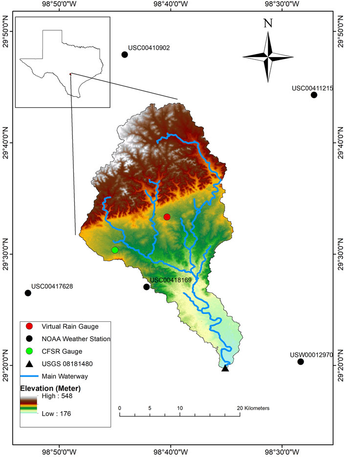
FIGURE 1. Location and digital elevation model of the Leon Creek Watershed (LCW) in Texas.

2.2 Data acquisition

Weather records from 1998 to 2009 of TRMM, CFSR, PRISM, and conventional rain gauges were collected to drive the hydrological models. The conventional weather gauge station data was obtained from the National Oceanic and Atmospheric Administration’s (NOAA) National Centers for Environmental Information (NCEI) climate data archive (https://www.ncdc.noaa.gov/cdo-web/search). A large number of weather stations have operated in the San Antonio region in the past. Nevertheless, only five stations proximate to LCW were found to have long-term precipitation records on a daily basis, none of which is physically located within the study watershed. The locations and station IDs of these five NOAA stations are shown in Figure 1. The precipitation, maximum, and minimum temperatures of the five stations were collected. The conventional gauge data was found to have multiple missing values during the study period, therefore, days with missing data were removed.

The CFSR weather data was downloaded from the Texas A&M University Global Weather Data for SWAT website (https://globalweather.tamu.edu/). The website provides CFSR data aggregated to a daily time step and interpolated to a SWAT input file format. The rectangular extent of the study watershed was used to extract the CFSR data. Within the study watershed, one CFSR gauge was available (Figure 1).

The TRMM and PRISM datasets were accessed using Google Earth Engine (GEE), a cloud-based geospatial analysis platform that provides easy access to many free geospatial data archives (Gorelick et al., 2017). The shapefile of the LCW was uploaded to the GEE platform to retrieve the pixels within the study watershed. The merged microwave/IR precipitation band of the TRMM 3B42 product at a 3-h temporal resolution was downloaded. The TRMM rainfall data was further aggregated into daily time steps for comparison with the other precipitation data sources at the same temporal resolution. The TRMM 3B42 3-Hourly Precipitation Estimates dataset has a spatial resolution of 2.5°. Additionally, the daily precipitation, mean, minimum, and maximum temperature are collected for the PRISM Daily Spatial Climate Dataset AN81d dataset, which has a much finer spatial resolution of 2.5 arc-minute. To enable comparison among the different data sources with different spatial resolutions, the GEE platform was used to conduct map algebra that calculates the areal-averaged weather data from TRMM and PRISM of the study watershed.

Other data required for this study was obtained from multiple sources. ANNs require only metrological data and streamflow observation for model training, whereas SWAT requires additional spatial characteristics data, including the digital elevation model (DEM), land use land cover (LULC) map, and soil map. In this work, the state soil geographic (STATSGO) database preloaded with the ArcSWAT interface was used as the soil map (Schwarz and Alexander, 1995). The National Elevation Dataset (NED) with 30 m resolution was used as the input DEM, and the 2011 National Land Cover Data Set (NLCD2011) was used as the LULC map. The NED and NLCD2011 datasets were accessed from the USDA Natural Resources Conversation Service (NRCS) geospatial data gateway (USDA-NRCS, 2014). In addition, the daily streamflow used for model calibration/training was obtained from USGS surface water gage 08181480 (U.S. Geological Survey, 2016) in Leon Creek from 2000 to 2009.

2.3 Hydrological simulations

2.3.1 SWAT modeling approach

This study used the ArcSWAT 2012 built for ArcGIS 10.5 to construct the rainfall-runoff model for LCW. First, a threshold of 1,500 ha was applied for stream definition. The threshold determines the minimum area for initiating stream networks. As a result, 25 subbasins were created. The study area was further discretized into 298 hydrological response units (HRUs) by applying a 10% threshold to remove minor slope, soil, and land cover classes. This procedure reduced the total number of HRUs, which improves computational efficiency. A detailed description of the SWAT modeling process can be found in the SWAT theoretical documentation (Neitsch et al., 2011).

The weather data sources discussed in Section 2.2 were used as the SWAT weather input. The CFSR and conventional gauge data were in point source format, the format of SWAT weather input files (Arnold et al., 2012). The longitude/latitude coordinates and elevation of the CFSR gauge and conventional gauges were directly used to create the precipitation and temperature files. The TRMM and PRISM data were originally in gridded format and converted into areal-averaged point source files using GEE. The location and elevation of the watershed centroid were obtained using ArcGIS and set as the “virtual rain gauge” (Elhassan et al., 2016), as displayed in Figure 1. In total, four SWAT modeling scenarios were created, SWAT-CFSR, SWAT-GAUGE, SWAT-TRMM, and SWAT-PRISM. The TRMM dataset only provides rainfall estimates; hence the temperature data from PRISM was used to drive the SWAT-TRMM model. Meanwhile, the temperature data from the other three sources were used to drive their corresponding modeling scenarios.

The four SWAT modeling scenarios were run for a 12-year simulation period on a daily time step. The year 1998–1999 was used for model warm-up, 2000 to 2006 was used for calibration, and 2007 to 2009 for model validation. The model calibration and validation processes were carried out in the SWAT Calibration and Uncertainty Programs (SWAT-CUP) using the SUFI-2 procedure. This study selected 15 parameters that are considered sensitive for streamflow simulation according to the literature (Arabi et al., 2007; Kim et al., 2015; Qi et al., 2017; Jimeno-Sáez et al., 2018; Koycegiz and Buyukyildiz, 2019; Chen et al., 2020). Their description and corresponding error range are summarized in Table 1.

TABLE 1

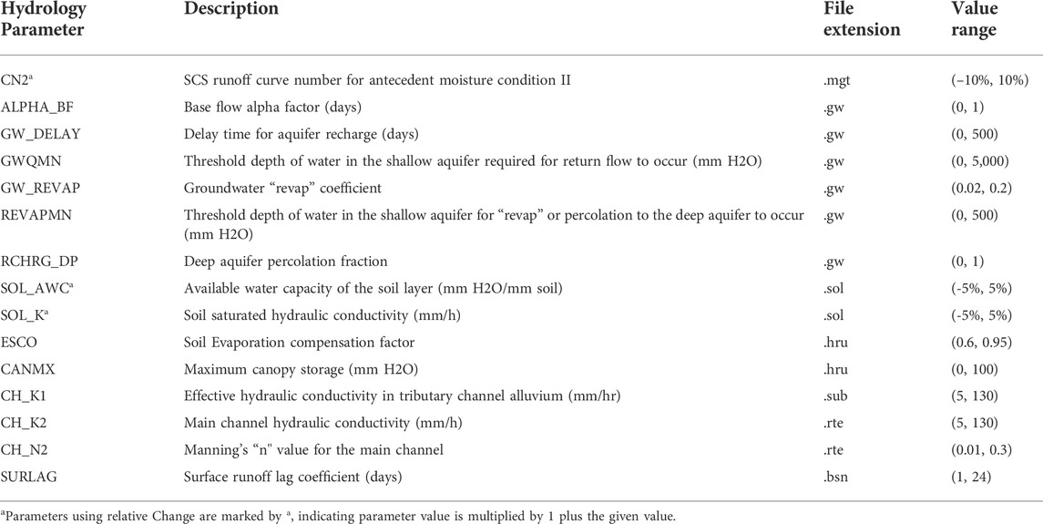
TABLE 1. Description of the calibrated SWAT parameters.

2.3.2 Artificial neural network modeling approach

A comprehensive review of the conception and application of ANNs as rainfall-runoff models can be found in ASCE (2000a) and ASCE (2000b). Three-layered feed-forward neural networks are widely applied in hydrological modeling and were used in this study. The ANNs use a training process to estimate free model parameters. Routinely, a range of neural networks with different structures is trained, after which a model selection process is implemented to determine the model that makes the best prediction outcome. In this study, three model structures that only utilize meteorological data as input were explored (Table 2). The input variables combinations were determined in reference to the review by Yaseen et al. (2015), which summarized the ANN model input combinations for streamflow forecasting of multiple previous studies. The ANN-TRMM, ANN-CFSR, ANN-PRISM, and ANN-GAUGE models were trained using weather inputs corresponding to each of the rainfall datasets. The Thiessen polygon method was applied to interpolate the weather observations from the five gauging stations to the areal-averaged data of LCW, which was used as input to the ANN models. Multiple missing dates were removed from model training for the ANN-GUAGE model. As for SWAT, the temperature data from the PRISM dataset was used in the ANN-TRMM model. The predictors included daily precipitation (P_t), precipitation of the previous n days (P_t-n), daily mean air temperature (T_t), and total precipitation for the preceding n days (P_n). The training target was observed streamflow (Q) at the watershed outlet. The back-propagation algorithm was used for model training, and the logistic function was set as the transfer function at the hidden layer units. All input variables and the training target are normalized to the range of 0–1 to speed up model training.

TABLE 2

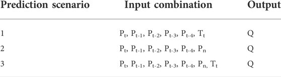
TABLE 2. ANN model input combinations.

In ANN rainfall-runoff modeling, too few hidden neurons may cause the model to fail to capture the complex nonlinear relationship between the predictors and targets, while too many hidden neurons can cause model overfitting (Demirel et al., 2009). In this work, the number of hidden layer units of all three input combinations was explored from 1 to 10, close to the experimental procedure of previous studies (Ha and Stenstrom, 2003; Kalin et al., 2010; Noori and Kalin, 2016). To select the best model among the trained models with different input combinations and hidden layer size, the Blocked Cross-Validation (BlockedCV) approach was applied with the root mean square error (RMSE) used as the model selection criteria. Cross-validation is the most widely used method for estimating prediction error in statistical modeling (Hastie et al., 2009). In rainfall-runoff modeling, the meteorological and hydrological data usually have strong autocorrelation and time dependency. BlockedCV groups the data points into sequentially consistent blocks and maintains sequential order within the blocks in the data splitting and cross-validation process (Bergmeir and Benítez, 2012). A more detailed description of the BlockedCV procedure conducted in this study is presented in Section 3.2.2. Data from 2000 to 2006 was used to train the model, and data from 2007 to 2009 was used for standalone model testing. The R software (R Core Team, 2019) was used for all ANN simulations in this study.

2.4 Precipitation and hydrological models evaluation

2.4.1 Rainfall products evaluation

The rainfall products comparison was conducted on the areal-averaged value of the study watershed, with calibration and validation phases evaluated independently. The Thiessen Polygon method areal-averaged precipitation from the conventional gauges, was compared with the other three gridded precipitation products. The relationship between the daily time series was evaluated using the Pearson correlation coefficient (CC) and percent bias (PBIAS), which mathematical formulation can be expressed in Eqs 1, 2:

$CC=\frac{COV\left(P_{grid},P_{gauge}\right)}{\sigma \left(P_{grid}\right)\sigma \left(P_{gauge}\right)}(1)$

$PBIAS=100\cdot \frac{{{\displaystyle \sum }}_i{\left(P_{grid}-P_{gauge}\right)}_i}{{{\displaystyle \sum }}_i{P}_{gauge,i}}(2)$

where $P_{grid}$ and $P_{gauge}$ denote the daily precipitation from the gridded weather products and conventional gauge data, respectively. The precipitation data were also aggregated to monthly resolution and evaluated graphically using box plots and scatter plots.

2.4.2 Hydrological models evaluation

The hydrological modeling results were evaluated using the Nash–Sutcliffe coefficient of efficiency (NSE) and percent bias (PBIAS). The NSE is a normalized statistic that determines the magnitude of residual variance compared to observed data variance. NSE ranges from –∞ to 1.0, with NSE = 1.0 representing the optimal fitting (Nash and Sutcliffe, 1970). The PBIAS measures the average tendency of model overestimation or underestimation. A smaller absolute PBIAS indicates better model fit to observed data. NSE and PBIAS were adopted in this study because they are commonly used in the literature, and extensive information regarding these two indicators is available from previous studies (Moriasi et al., 2015). The model performance evaluation criteria were adopted from (Moriasi et al., 2007), which recommended performance ratings for monthly time step hydrological simulations. Hydrological models are known to typically perform better at coarser temporal resolutions; hence, the performance ratings were slightly relaxed in this study (Kalin et al., 2010). The mathematical formulations of NSE and PBIAS and their corresponding performance criteria for daily streamflow simulation are presented in Table 3.

TABLE 3

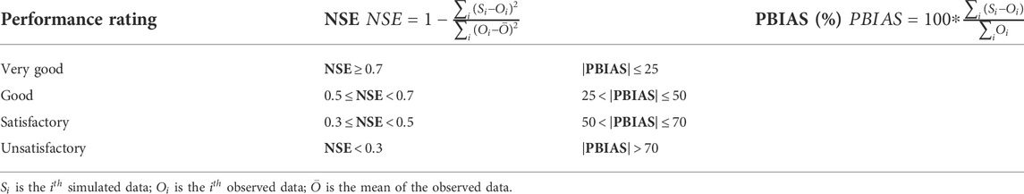
TABLE 3. Goodness-of-fit indicators and model performance evaluation criteria for the hydrological models.

3 Results and discussion

3.1 Precipitation data analysis

The areal-averaged gauge rainfall data from NOAA was used as the reference to analyze the precipitation of the three gridded weather datasets (TRMM, CFSR, and PRISM). Table 4 summarized the daily average precipitation depth (Mean), the standard deviation (Std), and the maximum daily precipitation (Max) of the four data sources. The correlation coefficient (CC) and percent bias (PBIAS) between the gridded rainfall data and the reference data are also presented. Since the conventional gauge precipitation records were incomplete during the study period, the missing dates were removed from all datasets for the calculation of CC and PBIAS.

TABLE 4

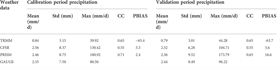
TABLE 4. Statistical summary of all precipitation data and comparison between the areal-averaged gridded rainfall with conventional gauges data.

The statistical summary shows that the daily rainfall during the calibration and validation periods are close in magnitude. The TRMM data had the lowest mean, maximum, and standard deviation of the rainfall, significantly lower than the estimates from the CFSR, PRISM, and conventional gauge data. However, the mean daily rainfall values from the CFSR, PRISM, and conventional gauge datasets were relatively close. The CFSR data had the highest average daily rainfall estimation (2.56 mm/d) for the calibration period, while in the validation period, the gauge data has the highest average daily value (2.44 mm/d). The PRISM data had the highest estimates of the maximum daily rainfall for both the calibration (180.92 mm/d) and validation periods (173.79 mm/d), and the largest standard deviations (8.75 mm for calibration and 9.52 mm for validation period). The CC values indicated that the PRISM data has the strongest correlation with the conventional gauge data among the three gridded rainfall datasets, and the CFSR data has the weakest correlation. The TRMM data has relatively strong correlation with the gauge rainfall data despite of its severe underestimation. It can therefore be assumed that the TRMM rainfall estimates capture the timing of the precipitation events quite well although missing their precise magnitudes. The PBIAS values agree with the daily mean estimates that the TRMM estimation of daily precipitation was significantly lower than that from gauge observation. Meanwhile, the CFSR and PRISM estimation of daily rainfall was slightly higher than the gauge observation.

Furthermore, the precipitation data were aggregated to the monthly time step to make graphical comparisons. The box plots of the aggregated monthly precipitation value of the four precipitation data sources are displayed in Figure 2. Some of the extremely high values were removed when creating the box plots to make the figure more readable. In both the calibration and validation periods, the TRMM 3B42 product had the lowest estimate of the median, lower and upper quartiles, and maximum values. In the calibration period, the monthly median rainfall estimation from CFSR (45.15 mm), PRISM (52.64 mm), and conventional gauge (52.51 mm) were relatively close compared with that from TRMM (16.98 mm). In the validation period, the PRISM data provided the highest estimates of median monthly precipitation of 46.68 mm, while the CFSR (31.14 mm) and conventional gauge (33.63 mm) had similar but smaller estimates.

FIGURE 2

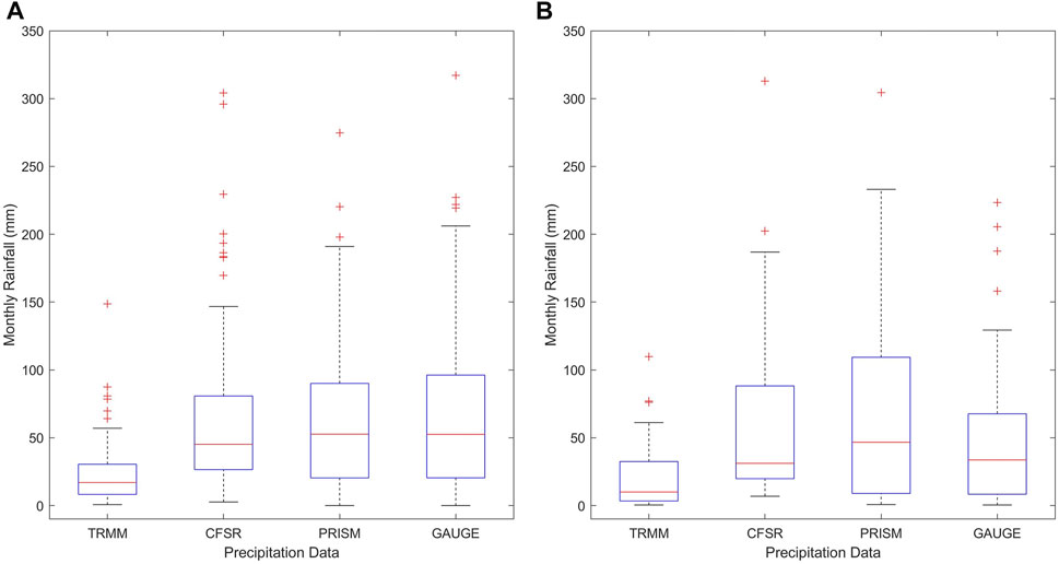
FIGURE 2. Monthly precipitation of TRMM, CFSR, PRISM, and conventional gauge for the (A) calibration and (B) validation period.

The scatter plots that compare aggregated monthly TRMM, CFSR, and PRISM precipitation data with the conventional gauge reference data are presented in Figure 3. In agreement with the results suggested by Table 4 and Figure 2, the least square regression lines for the TRMM data (Figures 3A,D) have slopes that are significantly lower than that for the CFSR and PRISM data (Figures 3B,C,E,F), which indicates substantial underestimation of precipitation. Meanwhile, the least square regression lines for the CFSR and PRISM data were closer to the 1:1 reference line, indicating a closer approximation between these two datasets with the reference data. In particular, the PRISM data points (Figures 3C,F) were distributed nearer to the 1:1 reference line, while the CFSR data points (Figures 3B,E) were spread further apart, suggesting the PRISM data better approximates the gauge observations.

FIGURE 3

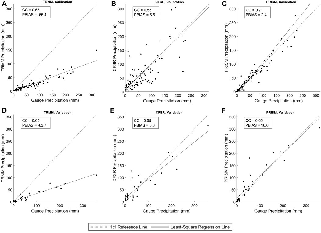
FIGURE 3. Comparison of the gridded monthly precipitation estimates with the conventional gauge data of the calibration period (A) TRMM, (B) CFSR, and (C) PRISM data; and the validation period (D) TRMM, (E) CFSR, and (F) PRISM data.

3.2 Hydrological simulations

3.2.1 Soil and water assessment tool calibration and validation

SWAT calibration results are conditioned on the selected procedure, objective function, and availability of data over the time period (Abbaspour, 2011). The iterative SUFI-2 procedure was used in this study, and 500 simulations were run in each calibration iteration. The parameter values were updated after each iteration, and the iterations ended after the objective function ceased to improve. The Nash-Sutcliffe Coefficient of Efficiency (NSE) was used as the objective function. The four modeling scenarios were calibrated against the observed daily streamflow at the watershed outlet, and separate calibrations were made for each scenario. The calibration process minimized the difference between simulated and observed streamflow (Abbaspour et al., 2018). The last iteration of the calibration was used to define the parameter output ranges, which were used in the corresponding validation iterations without further modification. The calibration outcome and the best-fitted value in the validation iteration were presented in Table 5.

TABLE 5

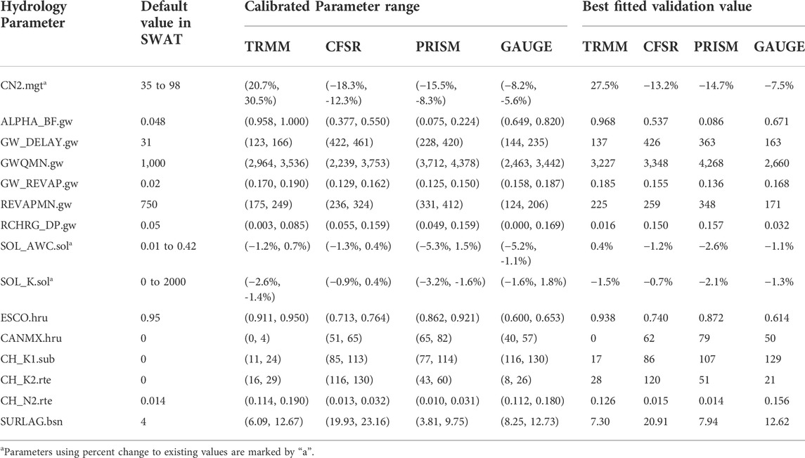
TABLE 5. Calibrated SWAT parameter ranges and the best-fitted validation values.

The SCS (Soil Conservation Service, the United States Department of Agriculture) runoff curve number (CN2.mgt) was reduced in the SWAT-CFSR, SWAT-PRISM, and SWAT-GAUGE models but significantly increased in the SWAT-TRMM model, compensating its lower precipitation. Similarly, the maximum canopy storage (CANMX.hru) of SWAT-TRMM was kept at 0, while in other models, the CANMX.hru value was increased by different extents from the default. The hydraulic conductivity of the tributary channel (CH_K1.sub) and main channel (CH_K2.rte) for the SWAT-TRMM model was notably lower than the other models, while the Manning’s n, the coefficient for the main channel (CH_N2.rte), which represents the roughness of the channel, was higher in the SWAT-TRMM model. The adjustments conducted on the channel-related parameters reduce streamflow velocity in the SWAT-TRMM model compared to the other models. The soil parameters were adjusted through a percent change due to their spatial heterogeneity. In this study, the available water capacity of the soil layer (SOL_AWC.sol) and the soil saturated hydraulic conductivity (SOL_K.sol) were only slightly adjusted for all four SWAT modeling scenarios, which indicated that the streamflow was not sensitive to soil parameters in the study watershed.

The groundwater parameters (.gw) govern the speed and volume of groundwater recharge and discharge in the study watershed, which can be vital to the simulation performance since the San Antonio region is situated above Edwards Aquifer, which stores an enormous amount of groundwater and supplies much of the municipal consumption for San Antonio (Loáiciga et al., 2000; Elhassan et al., 2016). The relatively large base flow alpha factor (ALPHA_BF.gw) for the SWAT-TRMM, SWAT-CFSR, and SWAT-GAUGE models suggests the study area’s groundwater has a rapid response to recharge. Furthermore, the higher than default groundwater “revap” coefficient (GW_REVAP.gw) indicates the water transfer from the shallow aquifer to the root zone occurs at a relatively high rate. Meanwhile, the threshold depth of water in the shallow aquifer required for return flow to occur (GWQMN.gw) was markedly increased from the default value for all SWAT model scenarios, which likely suggested the study area has a large water storage capacity in its shallow aquifer, typically of karstic geology. In addition, the delay time for aquifer recharge (GW_DELAY.gw) was increased from the default value for all modeling scenarios, suggesting a longer time for water to exit the soil profile and enters the shallow aquifer in the study area.

3.2.2 Artificial neural network training and model selection

All nodes in the neural networks were fully connected to nodes in their adjacent layers in this study. The links connecting the nodes contain weight and bias information which were optimized in the training process (ASCE, 2000a). The three-layer feed-forward neural network structure only contains one hidden layer besides the input and output layers. Thus, the primary purpose of the model selection process was to decide the number of hidden layer units that produces the best simulation outcome. As mentioned in Section 2.3.2, the available data was split 70/30 ratio into the training and testing groups, respectively. The training data was further divided into ten blocks. In each BlockedCV iteration, nine blocks were used for model training, while the other block was used to calculate cross-validation statistics. The root mean square error (RMSE) of the standalone block was calculated in each training cross-validation iteration. The RMSE values were averaged after the training iterations finished. The model with the smallest averaged RMSE was selected as the best model. The models that produce the smallest cross-validation RMSE for each prediction scenario are displayed in Table 6.

TABLE 6

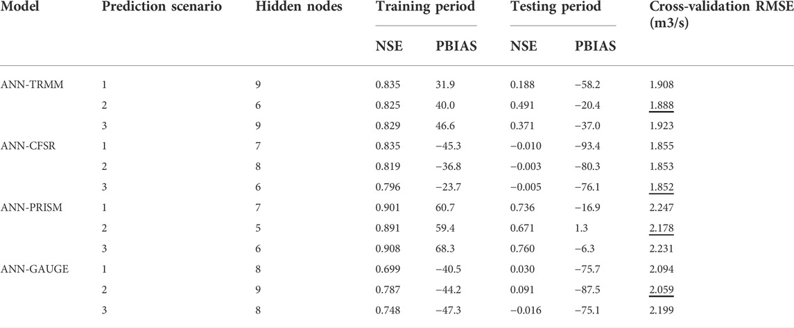
TABLE 6. Best model structure and performance results of all prediction scenarios.

The best models selected using the cross-validation RMSE as criteria had their hidden unit sizes that fell between 5 and 9. This finding is consistent with that of Wu et al. (2005), which found the size of the hidden units to be near two-thirds of the sum of the number of input and output neurons. The smallest cross-validation RMSE values for each model were highlighted with an underscore in Table 6. The ANN-TRMM, ANN-PRISM, and ANN-GAUGE models selected scenario 2 as having the best model input combination, which only used precipitation data as predictors. The ANN-CFSR model selected scenario 3 as the best input combination. The inclusion of temperature as one of the predictors had slightly improved the cross-validation performance of the ANN-CFSR model. Overall, the NSE and PBIAS values were close among the different prediction scenarios of a particular ANN model.

3.2.3 Comparison of model performance

The ANN models summarized in Table 6 were further screened based on the cross-validation RMSE, in which only one prediction scenario for each model was chosen as the best model. The best ANN models were compared with the calibrated SWAT models, and their goodness-of-fit indicators were summarized in Table 7. In the calibration period, the SWAT models’ NSE performance ranged from satisfactory to very good (0.48–0.90), and the ANN models’ NSE performance was all on the very good level (NSE ≥ 0.7). However, the PBIAS values of the calibration period suggested that the SWAT models, with the exception of the SWAT-TRMM model, overestimated streamflow. SWAT-TRMM, however, was the model which had the much smaller rainfall input. Similarly, the ANN models also showed notable forecasting bias. The ANN-TRMM and ANN-PRISM model overestimated the streamflow by over 40%, while the ANN-GAUGE model underestimated the streamflow by 44.2%.

TABLE 7

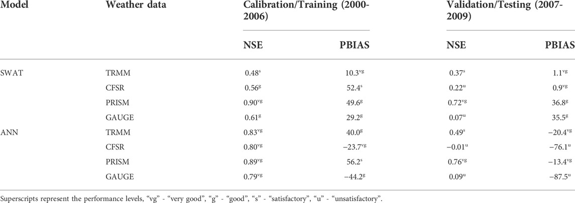
TABLE 7. Statistical performance of SWAT and ANN models driven by different weather data.

The hydrological models’ performance were worse in the validation period, during which only the TRMM and PRISM driven models reached at least a satisfactory level NSE performance. The SWAT-TRMM had a satisfactory validation NSE performance of 0.37, and the SWAT-PRISM model had a validation NSE value of 0.72, which was considered very good for daily streamflow simulation. Meanwhile, the validation NSE performance of SWAT-CFSR and SWAT-GAUGE models was below satisfactory level. Surprisingly, the SWAT-TRMM and SWAT-CFSR models had very minimal PBIAS values in the validation period, although not performing well based on the NSE criterion. Comparably, the ANN-TRMM model had a satisfactory performance of 0.49 NSE value, and the ANN-PRISM model had a very good performance of 0.76 NSE value, while the ANN-CFSR and ANN-GAUGE models performed poorly. Additionally, all ANN based models underestimated the streamflow according to the PBIAS values in the validation period, with ANN-CFSR and ANN-GAUGE severely underestimating streamflow, and ANN-TRMM and ANN-PRISM having a relatively a lower magnitude of underestimation.

The hydrographs of the validation period with precipitation records are displayed in Figure 4. Since gauge observations for much of the validation period were missing, there were several discontinuities in the ANN-GAUGE time series (Figure 4D) as no streamflow predictions were made on the missing dates. The observed streamflow time series suggests that the Leon Creek had close to 0 discharge volume for most of the validation period with only occasional moderate to high flows caused by intense storm events. In general, the TRMM and PRISM driven models captured the timing of major storm events rather well but had different levels of bias in flow magnitude (Figures 4A,C). The CFSR and conventional gauge driven models predicted the streamflow peaks poorly. The simulated streamflow time series also showed that the SWAT models generally made higher peak discharge estimations than the ANN models.

FIGURE 4

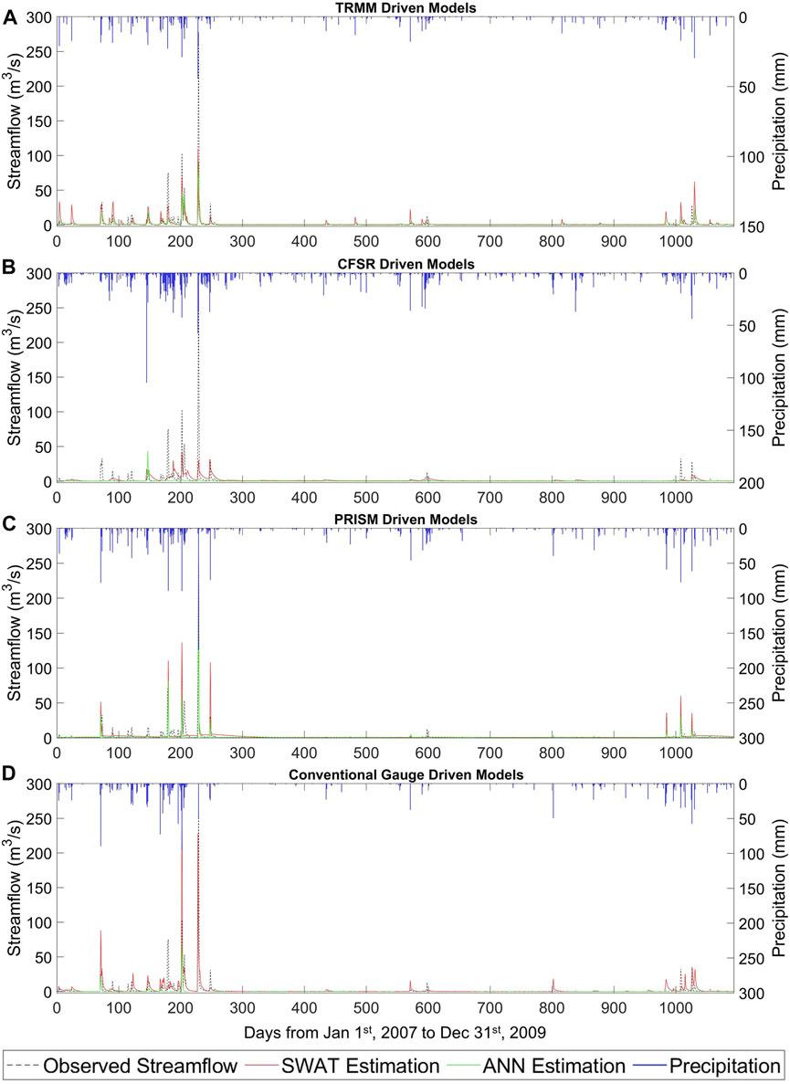
FIGURE 4. Hydrograph of the validation period for (A) TRMM, (B) CFSR, (C) PRISM, and (D) conventional gauge-driven SWAT and ANN models.

A scatter plot comparison of the simulated versus observed streamflow for the models driven by the different weather data sources is shown in Figure 5. The deviation of streamflow prediction increased with increasing discharge magnitude for all ANN and SWAT models. The SWAT-PRISM and ANN-PRISM models had least square regression lines comparably close to the 1:1 reference line, suggesting a smaller deviation between the simulated and observed data than other models. Meanwhile, the ANN-CFSR and ANN-GAUGE models were found to severely underpredict the streamflow with an extremely small regression line slope, which is in agreement with the PBIAS findings presented in Table 7. The regression line slope for all SWAT models was below that of the 1:1 reference line, which contradicts the PBIAS results that SWAT models overpredicted the streamflow. A very few underpredicted high flow values could be the cause of the small regression slope of the SWAT models, indicating the SWAT models overestimated low flows but underestimated high flows.

FIGURE 5

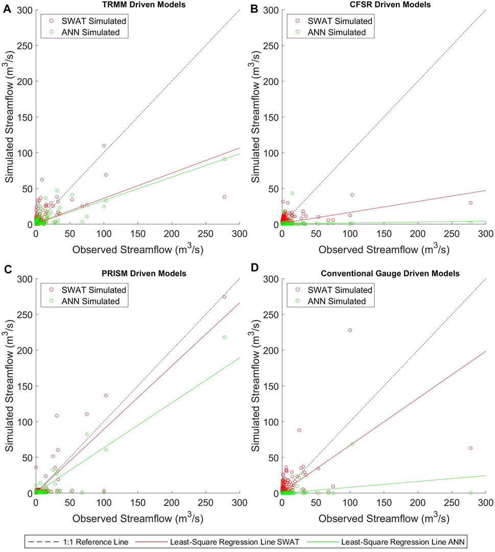
FIGURE 5. Comparison of validation period simulated and observed streamflow of the (A) TRMM, (B) CFSR, (C) PRISM, and (D) conventional gauge-driven models.

Overall, the performance of hydrological models in the standalone validation/testing period showed that the SWAT model overpredicted the streamflow and the ANN models underpredicted the streamflow for all evaluated weather data sources. The apparent underestimation made by the ANN models could be attribute to their training patterns, in which the overwhelming amount of low flow days in the training series caused the tendency of making lower estimations. The PRISM data was found to provide the most accurate hydrological simulations for both SWAT and ANN. The TRMM data also had satisfactory hydrological simulation performance, although NSE values were not as good as the PRISM-driven models.

The CFSR and conventional gauge driven models performed poorly according to the goodness-of-fit indicators and graphical comparison. This finding is unexpected given the common knowledge that rain gauges provide the most accurate precipitation measurement. These results are likely due to the lack of spatial representation of rain gauges and CFSR data in the study watershed. The five conventional rain gauges that had usable data in the region were spread outside the LCW boundary. Interpolating the rainfall data to the study area may fail to produce precise spatial representation. Another possible factor for the rain gauge-driven models’ failure is that temporal inconsistencies of gauge rainfall observations restrict the hydrological models’ prediction capability. This is particularly true for the ANN-GAUGE model, in which the temporal inconsistencies in input data undermine the time-dependent nature of streamflow series forecasting simulations. The CFSR data was initially in gridded format but automatically interpolated to the centroid point of the grid cell (Dile and Srinivasan, 2014), which also lacks an accurate representation of the study watershed. On the other hand, the TRMM and PRISM data were precisely extracted and averaged for the study watershed. By comparing the models driven by different weather data sources, it can therefore be assumed that the areal-averaged rainfall data input at the “virtual rain gauge” (watershed centroid) is a viable option for making good streamflow simulations in SWAT and ANN. Moreover, no significant discrepancy was found between SWAT and ANN simulation results when the same weather data source was used in the two models. At the same time, both models were greatly affected by the quality of precipitation inputs, and the results from the two models varied in the same way when different precipitation data sources were used.

4 Conclusion

SWAT and ANN are two widely used tools for streamflow prediction in the hydrological science community. This study evaluated the ability of four weather data sources to represent precipitation and drive hydrological simulations in a small urban watershed in central south Texas. The four different weather sources were directly compared on daily and monthly time steps. Furthermore, four SWAT models were calibrated and validated, and a number of ANN models were trained and selected to assess the relative performance of these different weather sources. Finally, goodness-of-fit indicators and graphical comparisons were employed to evaluate the results of hydrological simulations and further evaluate the different weather data source performance. The conclusions of this study can be summarized as follows:

1) The Thiessen polygon method was adopted to interpolate areal-averaged gauge rainfall for the study watershed. Using the interpolated gauge rainfall as reference data, the TRMM data was found to severely underestimate rainfall, while the PRISM data most closely approximated the gauge observations.

2) Only meteorological data was applied as the ANN model inputs. The ANN model selection results suggest that the precipitation data is adequate to make satisfactory streamflow prediction, except for the ANN-CFSR model, in which the addition of temperature as a predictor slightly improved the cross-validation RMSE performance.

3) The calibrated SWAT models and the selected best ANN models had satisfactory to very good model performance during the calibration/training period, while the model performance significantly reduced in the validation/testing period, with the exception of both PRISM driven models.

4) In the stand-alone validation/testing period, the PRISM data was found to provide the most accurate hydrological simulations for both SWAT and ANN. The TRMM data also had satisfactory level hydrological simulation performance. However, the CFSR and conventional gauge driven models performed poorly. The most likely explanation is that the interpolated CFSR and gauge rainfall data lacks spatial representation in the study watershed. Hence, the areal-averaged PRISM and TRMM data can offer a viable alternative for rainfall-runoff modeling when ground-based rainfall observation is limited.

5) The input of precipitation is vital for hydrological simulations, and both the SWAT and ANN models were strongly affected by the quality of precipitation inputs. Specifically, the SWAT and ANN models varied in an identical pattern when different precipitation data sources were used as inputs, and there was no significant discrepancy found between SWAT and ANN simulation results when the same weather data source was applied.

This work tested and verified the method of converting gridded format weather data into a point format for hydrological simulations via calculating their areal-averaged values. Converted meteorological data provided reliable inputs with the suitable format for the SWAT and ANN models and produced satisfactory streamflow simulation results. This method can be expanded into hydrological simulations using other lumped or semi-distributed models in the future, as more gridded weather products, either produced from satellite remote sensing techniques alone or created as hybrid ground-based measurement and remotely sensed estimates, are becoming publicly accessible. Moreover, due to the limitation of time and scope, this research only evaluated three common gridded-based precipitation datasets. Further research could also be conducted using radar estimated precipitation data that are gradually becoming available on a more refined spatial scale.

Data availability statement

The raw data supporting the conclusion of this article will be made available by the authors, without undue reservation.

Author contributions

XM and PS. contributed significantly to developing the methodology applied in this study. XM conducted the model simulations and wrote the original draft. XM PS JL and BL analyzed the results and revised the manuscript. All authors have read and agreed to the published version of the manuscript.

Funding

This research was supported by the International Joint Research Center for Smart Agriculture and Water Security of Yunnan Province research fund. The author XM was supported by the Texas A&M University Department of Water Management & Hydrological Science and the Department of Biological and Agricultural Engineering annual scholarship.

Acknowledgments

This manuscript is a chapter of the first author’s dissertation.

Conflict of interest

The authors declare that the research was conducted in the absence of any commercial or financial relationships that could be construed as a potential conflict of interest.

Publisher’s note

All claims expressed in this article are solely those of the authors and do not necessarily represent those of their affiliated organizations, or those of the publisher, the editors and the reviewers. Any product that may be evaluated in this article, or claim that may be made by its manufacturer, is not guaranteed or endorsed by the publisher.

References

Abbaspour, K. C. (2011). SWAT-CUP4: SWAT calibration and uncertainty programs–a user manual, 106. Eawag: Swiss Federal Institute of Aquatic Science and Technology.

Google Scholar

Abbaspour, K. C., Vaghefi, S. A., and Srinivasan, R. (2018). A guideline for successful calibration and uncertainty analysis for soil and water assessment: A review of papers from the 2016 international SWAT conference. Multidisciplinary Digital Publishing Institute. Basel, Switzerland.

Google Scholar

Adler, R. F., Huffman, G. J., Chang, A., Ferraro, R., Xie, P.-P., Janowiak, J., et al. (2003). The version-2 global precipitation climatology project (GPCP) monthly precipitation analysis (1979–present). J. Hydrometeorol. 4, 1147–1167. doi:10.1175/1525-7541(2003)004<1147:tvgpcp>2.0.co;2

CrossRef Full Text | Google Scholar

Ahmed, J. A., and Sarma, A. K. (2007). Artificial neural network model for synthetic streamflow generation. Water Resour. manage. 21, 1015–1029. doi:10.1007/s11269-006-9070-y

CrossRef Full Text | Google Scholar

Arabi, M., Govindaraju, R. S., and Hantush, M. M. (2007). A probabilistic approach for analysis of uncertainty in the evaluation of watershed management practices. J. Hydrology 333, 459–471. doi:10.1016/j.jhydrol.2006.09.012

CrossRef Full Text | Google Scholar

Arnold, J., Kiniry, J., Srinivasan, R., Williams, J., Haney, E., and Neitsch, S. (2012). Soil and water assessment tool, input/output documentation version 2012. College Station: Texas Water Resources Institute.

Google Scholar

ASCE (2000a). Artificial neural networks in hydrology. I: Preliminary concepts. J. Hydrol. Eng. 5, 115–123. doi:10.1061/(asce)1084-0699(2000)5:2(115)

CrossRef Full Text | Google Scholar

ASCE (2000b). Artificial neural networks in hydrology. II: Hydrologic applications. J. Hydrol. Eng. 5, 124–137. doi:10.1061/(asce)1084-0699(2000)5:2(124)

CrossRef Full Text | Google Scholar

Bergmeir, C., and Benítez, J. M. (2012). On the use of cross-validation for time series predictor evaluation. Inf. Sci. 191, 192–213. doi:10.1016/j.ins.2011.12.028

CrossRef Full Text | Google Scholar

Beven, K. J. (2011). Rainfall-runoff modelling: The primer. John Wiley & Sons. Hoboken, New Jersey, United States.

Google Scholar

Cepeda, J. C. (2017). Influence of pacific sea surface temperatures on precipitation in Texas: Data from amarillo and san antonio, 1900-2013. Tex. J. Sci. 69 (1), 67–80.

Google Scholar

Chen, M., Gassman, P. W., Srinivasan, R., Cui, Y., and Arritt, R. (2020). Analysis of alternative climate datasets and evapotranspiration methods for the Upper Mississippi River Basin using SWAT within HAWQS. Sci. Total Environ. 720, 137562. doi:10.1016/j.scitotenv.2020.137562

PubMed Abstract | CrossRef Full Text | Google Scholar

Daly, C., Halbleib, M., Smith, J. I., Gibson, W. P., Doggett, M. K., Taylor, G. H., et al. (2008). Physiographically sensitive mapping of climatological temperature and precipitation across the conterminous United States. Int. J. Climatol. 28, 2031–2064. doi:10.1002/joc.1688

CrossRef Full Text | Google Scholar

Demirel, M. C., Venancio, A., and Kahya, E. (2009). Flow forecast by SWAT model and ANN in Pracana basin, Portugal. Adv. Eng. Softw. 40, 467–473. doi:10.1016/j.advengsoft.2008.08.002

CrossRef Full Text | Google Scholar

Dile, Y. T., and Srinivasan, R. (2014). Evaluation of CFSR climate data for hydrologic prediction in data‐scarce watersheds: An application in the blue nile River Basin. J. Am. Water Resour. Assoc. 50, 1226–1241. doi:10.1111/jawr.12182

CrossRef Full Text | Google Scholar

Elhassan, A., Xie, H., Al-Othman, A. A., Mcclelland, J., and Sharif, H. O. (2016). Water quality modelling in the San Antonio River Basin driven by radar rainfall data. Geomatics, Nat. Hazards Risk 7, 953–970. doi:10.1080/19475705.2015.1009500

CrossRef Full Text | Google Scholar

Fuka, D. R., Walter, M. T., Macalister, C., Degaetano, A. T., Steenhuis, T. S., Easton, Z. M., et al. (2014). Using the Climate Forecast System Reanalysis as weather input data for watershed models. Hydrol. Process. 28, 5613–5623. doi:10.1002/hyp.10073

CrossRef Full Text | Google Scholar

Gao, J., Sheshukov, A. Y., Yen, H., and White, M. J. (2017). Impacts of alternative climate information on hydrologic processes with SWAT: A comparison of NCDC, PRISM and NEXRAD datasets. Catena 156, 353–364. doi:10.1016/j.catena.2017.04.010

CrossRef Full Text | Google Scholar

Gassman, P. W., Reyes, M. R., Green, C. H., and Arnold, J. G. (2007). The soil and water assessment tool: Historical development, applications, and future research directions. Trans. ASABE 50, 1211–1250. doi:10.13031/2013.23637

CrossRef Full Text | Google Scholar

Geological Survey, U. S. (2016). National water information system data available on the world wide web (USGS water data for the nation). [Online]. Available at: https://waterdata.usgs.gov/nwis (Accessed April 24, 2020).

Google Scholar

Gorelick, N., Hancher, M., Dixon, M., Ilyushchenko, S., Thau, D., Moore, R., et al. (2017). Google Earth engine: Planetary-scale geospatial analysis for everyone. Remote Sens. Environ. 202, 18–27. doi:10.1016/j.rse.2017.06.031

CrossRef Full Text | Google Scholar

Govindaraju, R. S., and Rao, A. R. (2013). Artificial neural networks in hydrology. Springer Science & Business Media. Berlin/Heidelberg, Germany.

Google Scholar

Guo, J., Liang, X., and Leung, L. R. (2004). Impacts of different precipitation data sources on water budgets. J. Hydrology 298, 311–334. doi:10.1016/j.jhydrol.2003.08.020

CrossRef Full Text | Google Scholar

Ha, H., and Stenstrom, M. K. (2003). Identification of land use with water quality data in stormwater using a neural network. Water Res. 37, 4222–4230. doi:10.1016/s0043-1354(03)00344-0

PubMed Abstract | CrossRef Full Text | Google Scholar

Hastie, T., Tibshirani, R., and Friedman, J. (2009). The elements of statistical learning: Data mining, inference, and prediction. Springer Science & Business Media. Berlin/Heidelberg, Germany.

Google Scholar

Himanshu, S. K., Pandey, A., and Patil, A. (2018). Hydrologic evaluation of the TMPA-3B42V7 precipitation data set over an agricultural watershed using the SWAT model. J. Hydrol. Eng. 23, 05018003. doi:10.1061/(asce)he.1943-5584.0001629

CrossRef Full Text | Google Scholar

Jimeno-Sáez, P., Senent-Aparicio, J., Pérez-Sánchez, J., and Pulido-Velazquez, D. (2018). A Comparison of SWAT and ANN models for daily runoff simulation in different climatic zones of peninsular Spain. Water 10, 192. doi:10.3390/w10020192

CrossRef Full Text | Google Scholar

Kalin, L., Isik, S., Schoonover, J. E., and Lockaby, B. G. (2010). Predicting water quality in unmonitored watersheds using artificial neural networks. J. Environ. Qual. 39, 1429–1440. doi:10.2134/jeq2009.0441

PubMed Abstract | CrossRef Full Text | Google Scholar

Kim, M., Baek, S., Ligaray, M., Pyo, J., Park, M., Cho, K., et al. (2015). Comparative studies of different imputation methods for recovering streamflow observation. Water 7, 6847–6860. doi:10.3390/w7126663

CrossRef Full Text | Google Scholar

Koycegiz, C., and Buyukyildiz, M. (2019). Calibration of SWAT and two data-driven models for a data-scarce mountainous headwater in semi-arid Konya closed basin. Water 11, 147. doi:10.3390/w11010147

CrossRef Full Text | Google Scholar

Li, D., Christakos, G., Ding, X., and Wu, J. (2018). Adequacy of TRMM satellite rainfall data in driving the SWAT modeling of Tiaoxi catchment (Taihu lake basin, China). J. Hydrology 556, 1139–1152. doi:10.1016/j.jhydrol.2017.01.006

CrossRef Full Text | Google Scholar

Loáiciga, H., Maidment, D., and Valdes, J. B. (2000). Climate-change impacts in a regional karst aquifer, Texas, USA. J. Hydrology 227, 173–194. doi:10.1016/s0022-1694(99)00179-1

CrossRef Full Text | Google Scholar

Mararakanye, N., le Roux, J., and Franke, A. (2020). Using satellite-based weather data as input to SWAT in a data poor catchment. Phys. Chem. Earth, Parts A/B/C 117, 102871. doi:10.1016/j.pce.2020.102871

CrossRef Full Text | Google Scholar

Minns, A., and Hall, M. (1996). Artificial neural networks as rainfall-runoff models. Hydrological Sci. J. 41, 399–417. doi:10.1080/02626669609491511

CrossRef Full Text | Google Scholar

Moriasi, D. N., Arnold, J. G., van Liew, M. W., Bingner, R. L., Harmel, R. D., Veith, T. L., et al. (2007). Model evaluation guidelines for systematic quantification of accuracy in watershed simulations. Trans. ASABE 50, 885–900. doi:10.13031/2013.23153

CrossRef Full Text | Google Scholar

Moriasi, D. N., Gitau, M. W., Pai, N., and Daggupati, P. (2015). Hydrologic and water quality models: Performance measures and evaluation criteria. Trans. ASABE 58, 1763–1785. doi:10.13031/trans.58.10715

CrossRef Full Text | Google Scholar

Muche, M. E., Sinnathamby, S., Parmar, R., Knightes, C. D., Johnston, J. M., Wolfe, K., et al. (2019). Comparison and evaluation of gridded precipitation datasets in a Kansas agricultural watershed using SWAT. J. Am. Water Resour. Assoc. 56, 486–506. doi:10.1111/1752-1688.12819

CrossRef Full Text | Google Scholar

Nash, J. E., and Sutcliffe, J. V. (1970). River flow forecasting through conceptual models part I—a discussion of principles. J. hydrology 10, 282–290. doi:10.1016/0022-1694(70)90255-6

CrossRef Full Text | Google Scholar

Neitsch, S. L., Arnold, J. G., Kiniry, J. R., and Williams, J. R. (2011). Soil and water assessment tool theoretical documentation version 2009. College Station: Texas Water Resources Institute.

Google Scholar

Noori, N., and Kalin, L. (2016). Coupling SWAT and ANN models for enhanced daily streamflow prediction. J. Hydrology 533, 141–151. doi:10.1016/j.jhydrol.2015.11.050

CrossRef Full Text | Google Scholar

Ochoa, A., Pineda, L., Crespo, P., and Willems, P. (2014). Evaluation of TRMM 3B42 precipitation estimates and WRF retrospective precipitation simulation over the Pacific–Andean region of Ecuador and Peru. Hydrol. Earth Syst. Sci. 18, 3179–3193. doi:10.5194/hess-18-3179-2014

CrossRef Full Text | Google Scholar

Qi, Z., Kang, G., Chu, C., Qiu, Y., Xu, Z., Wang, Y., et al. (2017). Comparison of SWAT and GWLF model simulation performance in humid south and semi-arid north of China. Water 9, 567. doi:10.3390/w9080567

CrossRef Full Text | Google Scholar

R CORE TEAM (2019). R: A language and environment for statistical computing. R Found. Stat. Comput. 1. doi:10.1890/0012-9658(2002)083[3097:CFHIWS]2.0.CO;2

CrossRef Full Text | Google Scholar

Radcliffe, D., and Mukundan, R. (2017). PRISM vs. CFSR precipitation data effects on calibration and validation of SWAT models. J. Am. Water Resour. Assoc. 53, 89–100. doi:10.1111/1752-1688.12484

CrossRef Full Text | Google Scholar

Roth, V., and Lemann, T. (2016). Comparing CFSR and conventional weather data for discharge and soil loss modelling with SWAT in small catchments in the Ethiopian Highlands. Hydrol. Earth Syst. Sci. 20, 921–934. doi:10.5194/hess-20-921-2016

CrossRef Full Text | Google Scholar

Saha, S., Moorthi, S., Wu, X., Wang, J., Nadiga, S., Tripp, P., et al. (2014). The NCEP climate forecast system version 2. J. Clim. 27, 2185–2208. doi:10.1175/jcli-d-12-00823.1

CrossRef Full Text | Google Scholar

Schwarz, G. E., and Alexander, R. (1995). State soil geographic (STATSGO) data base for the conterminous United States.

Google Scholar

Srivastava, P., Mcnair, J. N., and Johnson, T. E. (2006). Comparison of process based and artificial neural network approaches for streamflow modeling in an agricultural watershed. J. Am. Water Resour. Assoc. 42, 545–563. doi:10.1111/j.1752-1688.2006.tb04475.x

CrossRef Full Text | Google Scholar

Stampoulis, D., and Anagnostou, E. N. (2012). Evaluation of global satellite rainfall products over continental Europe. J. Hydrometeorol. 13, 588–603. doi:10.1175/jhm-d-11-086.1

CrossRef Full Text | Google Scholar

Tuppad, P., Douglas-Mankin, K., Lee, T., Srinivasan, R., and Arnold, J. (2011). Soil and Water Assessment Tool (SWAT) hydrologic/water quality model: Extended capability and wider adoption. Trans. ASABE 54, 1677–1684. doi:10.13031/2013.39856

CrossRef Full Text | Google Scholar

USDA-NRCS (2014). Geospatial data gateway. [Online]. Available at: https://datagateway.nrcs.usda.gov/ (Accessed April 20, 2020).

Google Scholar

Worqlul, A. W., Maathuis, B., Adem, A. A., Demissie, S. S., Langan, S., Steenhuis, T. S., et al. (2014). Comparison of rainfall estimations by TRMM 3B42, MPEG and CFSR with ground-observed data for the Lake Tana basin in Ethiopia. Hydrol. Earth Syst. Sci. 18, 4871–4881. doi:10.5194/hess-18-4871-2014

CrossRef Full Text | Google Scholar

Wu, J. S., Han, J., Annambhotla, S., and Bryant, S. (2005). Artificial neural networks for forecasting watershed runoff and stream flows. J. Hydrol. Eng. 10, 216–222. doi:10.1061/(asce)1084-0699(2005)10:3(216)

CrossRef Full Text | Google Scholar

Yaseen, Z. M., El-Shafie, A., Jaafar, O., Afan, H. A., and Sayl, K. N. (2015). Artificial intelligence based models for stream-flow forecasting: 2000–2015. J. Hydrology 530, 829–844. doi:10.1016/j.jhydrol.2015.10.038

CrossRef Full Text | Google Scholar

Yen, H., Daggupati, P., White, M. J., Srinivasan, R., Gossel, A., Wells, D., et al. (2016). Application of large-scale, multi-resolution watershed modeling framework using the hydrologic and water quality system (HAWQS). Water 8, 164. doi:10.3390/w8040164

CrossRef Full Text | Google Scholar

Zakizadeh, H., Ahmadi, H., Zehtabian, G., Moeini, A., and Moghaddamnia, A. (202010289). A novel study of SWAT and ANN models for runoff simulation with application on dataset of metrological stations. Phys. Chem. Earth. Parts A/B/C. 120, 102899, doi:10.1016/j.pce.2020.102899

CrossRef Full Text | Google Scholar