Stereo Thermal Marking Velocimetry

This paper presents a novel approach to measuring and mapping shape and motion of the water surface. The approach combines and borrows from existing techniques, such as stereo imaging shape recognition and tracking, infrared (IR) laser marking and thermography, and particle image velocimetry. The system consists of a high power IR laser beam controlled by a programmable marking head and two IR cameras tracking the thermal pattern projected by the beam onto the water surface. The paper provides detailed description of the setup, discusses the choice of the thermal pattern, and describes the IR image processing algorithm. An example of resolved surface shape and velocity maps is given for an experiment conducted in a laboratory wave tank.

Introduction

Water flow measurements near the wavy air–sea interface are notoriously difficult. It is the most energetic and violent part of the water column, introducing much stress and occasionally exposing to air any attempted sensor setup. Furthermore, cyclical nature of the wave orbital motion often brings turbulent wake behind the sensor and its platform back into the sampling volume of the sensor. Combined, these effects reliably contaminate most attempts at delicate in situ turbulence measurements, leaving an important gap in our empirical understanding of the turbulent microstructure within the top few meters of the upper ocean mixed layer. This motivates the development of remote, non-intrusive sensing methods for sampling the motion of the upper ocean, one of which is described in this paper.

The advances in sensitivity, sensor resolution, and commercial availability of mid- and long-wave infrared (IR) cameras in the past two decades paved the way for several investigators to take advantage and discover the utility of this remote sensing modality for visualizing horizontal spatial structure of near-surface flows with unmatched clarity and detail. First, Melville et al. (1998), then more recently Handler et al. (2001, 2012), Zhang and Harrison (2004), Garbe et al. (2004), and Handler and Smith (2011) investigated various aspects of wind and wave driven surface turbulence in wind–wave laboratory tanks. In the field, this work was expanded further by Sutherland (2013) and Sutherland and Melville (2013, 2015a,b) with a stereo IR setup on R/P FLIP. Airborne IR imagery has been used extensively by Marmorino et al. (2004, 2005, 2009, 2010, 2015); Marmorino and Smith, 2007 and Savelyev et al. (2018) to observe upper ocean turbulence on slightly larger scales ranging from meters to submesoscales.

Mid- and long-wave IR cameras are typically sensitive to radiation with wavelength ranges anywhere between 3 and 14 µm, where water absorption is very effective, and so the measured signal corresponds to the water skin temperature only within the top few tens of microns. The reason the studies listed above were able to observe much deeper turbulent eddies and other flow features is because they work on stretching and compressing the thermal skin layer, thus modulating the skin temperature and leaving a surface thermal footprint of an underlying process for the IR camera to see. The availability of this effective remote sensing tool is, of course, very fortunate. Its shortcomings, however, are rarely discussed. Meanwhile, the signal to noise ratio within an imaged IR scene, and hence the success of a set of IR observations, strongly depend on the magnitude of the temperature difference across the thermal skin layer, which is rarely known and even less so controlled. It is the conditions where the total air–sea heat flux is high and the small-scale subsurface turbulent mixing is weak that tend to result in strong thermal skin layer development and thus successful flow visualization with an IR camera. However, such conditions are not always in place; therefore, to some extent, most passive IR imaging studies are opportunistic in their nature. Moreover, without resolving the physics of the thermal skin layer, the magnitude of the IR signal often bears only qualitative meaning and cannot be directly converted to the magnitude of underlying currents.

Another source of concern for an IR observer is the level of noise, especially in situations where the available skin temperature variability is weak. While the internal noise equivalent delta temperature of a modern IR camera can be very low (<20 mK), the variability in downwelling radiation reflected from the water surface into the view of the camera can far exceed that. In the field, the direct sun glint oversaturates the sensor, but even at night, the reflections of the sky or of a nearby platform from various facets of surface waves can compete with the useful signal. Even in the laboratory conditions, this can present a problem if the background radiation is not uniform.

The need to overcome some of the passive IR imaging limitations and to boost and control the available signal motivated the development of active IR imaging techniques. While there are many ways in which one can introduce heat into the field of view, most of them would either distort the flow or at least introduce unwanted and poorly controlled heterogeneity. It was realized early on that a laser beam is by far the most efficient and precise tool. Particularly, the commonly available CO₂ laser emitting at 10.6 µm wavelength is ideal, because it deposit all of its energy into heat within the top few tens of microns of the water column for the IR camera to see. Moreover, because CO₂ lasers are often used in engraving applications, they can come integrated with a marking head, allowing for rapid reorientation of the beam angle, and thus an arbitrary thermal pattern can be drawn on the water surface.

Early utilization of CO₂ lasers for water surface studies, and particularly for air–sea heat and gas exchange measurements started in combination with single point radiometers (Jähne et al., 1989) and continued once first imagers became widely available (Haußecker et al., 1998). Soon after, it was realized that warm markers can be tracked between consecutive IR images to reliably and repeatedly obtain surface velocities at desired locations. Such studies were conducted both in wind–wave tunnels (Veron and Melville, 2001, Savelyev et al., 2012) and in the field on R/P FLIP (Veron et al., 2008, 2009).

Motivated by the success of these recent studies, this paper describes further development of active IR imaging methods. The method described here combines the idea of active thermal marking (so far only done with single camera) with the stereo IR imaging (so far only done passively) to create a Stereo Thermal Marking Velocimetry (STMV) system. The focus of the paper is on methodology of STMV, which goes into details and tradeoffs of the hardware needed for the system, and of the image processing algorithm used to reconstruct 3D geometry of the surface displacement and surface velocity. An example of the flow field resolved by the system in a laboratory wave tank is shown in results, followed by a discussion of sampling opportunities brought about by the new capability.

Methodology

The STMV system described here (Figure 1) consists of a CO₂ laser emitting 100 W IR laser beam, which is directed by a 2-mirror marking head to draw and repeatedly refresh a desired thermal pattern on the water surface. Two IR cameras are viewing and recording images of the pattern from different angles in stereo mode. In image post-processing, features of the thermal pattern are recognized in each image pair and used to reconstruct their 3D coordinates. By locating and tracking a cloud of thermal markers, STMV is able to resolve both the shape and 3D velocity vectors of the water surface. Subchapters below provide details on each major component of this methodology.

FIGURE 1

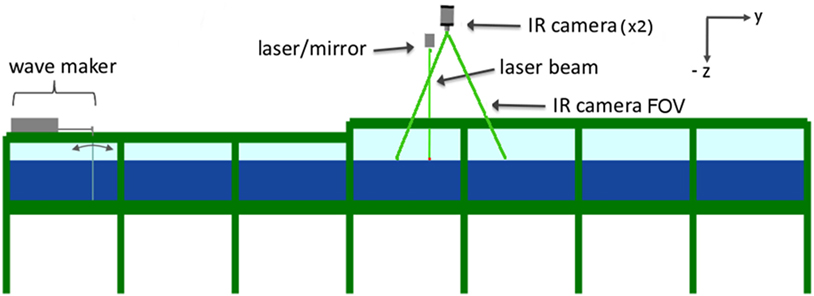
Figure 1. Side-view schematic of the experimental setup. An 8.5 m long and 2.3 m wide tank was filled with 0.5 m of water and equipped with a bottom-hinged wave maker at one end. The laser and both infrared (IR) cameras were located 3.6 m away from the wave maker and 1.9 m above the water level. Across-tank (x) distance between the two IR cameras was 1.4 m with both optical axes pointing slightly toward each other and intersecting approximately at the same location on the water surface at the centerline of the wave tank. Along-tank field of view (FOV) of IR cameras is shown with green lines.

Laser and Marking Head

The CO₂ laser is the heart of the STMV system. Generally, it is beneficial to have as much beam power as possible, limited only by the laser’s weight and form factors, power and cooling requirements, and most importantly laser safety considerations. Here, a 100 W, 10.6 µm water-cooled Synrad Pulstar p100 was used, which provided sufficient signal in continuous mode. The pulsing mode was reserved for situations where the thermal marker would get smeared due to noticeable surface motion during the laser dwell time; however, this was never the case. An important laser specification parameter is the beam divergence, in this case, 2.0 mrads, which determines the smallest size features the laser will be able to draw as a part of the thermal pattern. Small beam divergence also means more initial thermal signal available for the IR camera to detect, however, note, for similar reasons small divergence has a negative impact on laser safety calculations, causing a wider nominal hazard zone.

Upon exit from the laser, the laser beam immediately enters the Synrad FH Flyer marking head. It is equipped with two lightweight scan mirrors capable of changing 2D beam angle orientation at a rate exceeding >1 kHz. Upon the exit from the marking head, the laser beam would normally go through a focusing lens, which is not helpful at long range and was removed for the purposes of STMV. The mirrors are fully programmable and aligned with the laser by the manufacturer. Provided software WinMark Pro v6 allows creating new laser beam patterns or importing externally created patterns in an image format. Once the pattern is created, the software automatically optimizes beam path and synchronizes mirror and laser control signals to execute the pattern. The marking head allows for external trigger signal inputs and outputs, which can be programmed into the pattern execution sequence. This feature was used to synchronize thermal patterns with camera frames and shutters, as well as with the water wave generator.

IR Cameras

A large variety of IR cameras exists that are potentially suitable for STMV. The preferred camera choice is a mid-wave (3–5 µm) cooled Indium Antimonide (InSb) detector with as many pixels as possible. In this study, a camera with such sensor was available (FLIR SC6000), which has a superior thermal sensitivity of <18 mK and short integration time ~1.5–2 ms, allowing for >120 Hz frame rate. The sensor resolution was 640 × 512; however, 1 megapixel cameras are already available at this time and are preferred.

Long-wave IR cameras can also be used for STMV. In this example, the second camera was Sofradir Atom 1024 with a 1,024 × 768 uncooled ASi Microbolometer detector. Its thermal sensitivity is noticeably worse (<50 mK); however, it is still sufficient to detect and track thermal markers. A more significant limitation is 30 ms integration time, potentially causing some blurring of fast moving thermal markers, and capping the frame rate at 30 Hz. The biggest problem, however, is the camera’s sensitivity range of 8–14 µm, which captures CO₂ laser’s wavelength of 10.6 µm. Even a small amount of reflected laser beam energy can and will damage the sensor. Therefore, it has to be protected during the laser operation, which is a significant shortcoming. This can be accomplished with a filter, or as in this study with a mechanical shutter, which was controlled by a trigger output signal from the marking head.

Images from both cameras were grabbed via camera link ports and recorded in real time with an IO Industries CORE DVR system. The CORE is equipped with a raid system of four solid state hard drives, resulting in sufficient bandwidth (up to ~700 MB/s) and disk space (~1 TB) to record continuously for well over an hour. Furthermore, hard drives can be easily swapped if longer duration is needed.

Calibration

There is a variety of approaches one can attempt at calibrating a stereo imaging system to relate camera pixels to physical locations in 3D space. A well-known Caltech’s Camera Calibration Toolbox for Matlab^® requires multiple snapshots of a checker grid positioned at various angles within the field of view (FOV) of both cameras. A more straightforward approach would involve measuring all distances and angles to resolve the geometry of the setup and arrive at pixel locations directly. In the latter case, a snapshot of a calibration target is still desired for final adjustments to correct for measurement errors. The approach presented here requires neither setup geometry measurements nor a physical calibration target. Instead, it takes advantage of the availability of a perfectly leveled flat quiescent water surface in a laboratory wave tank and of the thermal laser capable of marking an arbitrary calibration target on that surface.

For a calibration target, the laser is programmed to make a regular spaced square grid of dots over the entire FOV, for example, as in Figure 2. This figure shows an IR image in binary format, which is an intermediate step of thermal mark detection described in more detail in Section “Image Processing Algorithm.” Due to the presence of IR noise, some grid points are clearly missing, while extras exist between regular spacing. A recursive algorithm of reconstructing and numbering rows and columns of the regular grid filters out such erroneous points.

FIGURE 2

Figure 2. White markers are a binary representation of an infrared image of a calibration pattern. Red circles are drawn around the exact centroid locations of detected markers.

Next step of the calibration is the lens distortion correction. Note, since the lens focus setting affects lens function and the final focus adjustment is often made after the camera has been mounted, it is desirable to make lens distortion correction a part of the calibration procedure for each setup. Once all pixel locations of thermal marks are defined, the lens distortion reveals itself by introducing bending to an otherwise straight and square calibration patter. This is especially evident along the edges of the image in Figure 2. Instead of defining a lens distortion model and looking for its coefficients, a more empirical and universally applicable approach is undertaken here. Since the distortion is the smallest in the center, a subset grid of points (7 × 7 in this case) in the center is used as a baseline. A series of straight lines are fitted through each row and each column within the subset to determine corrected locations of the grid throughout the image, Figure 3.

FIGURE 3

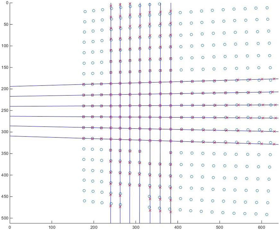
Figure 3. Linear fits through a 7 × 7 marker subset at the center shows the shift between distorted (circles) and corrected (crosses) location of thermal markers. Units correspond to raw image pixel numbers.

Deviations of markers from their expected location both in x and y directions give realizations of the desired lens distortion function throughout the image. Based on these realizations, 3D cubic polynomials are formed (Figure 4) for x and y coordinates, which is the desired result used later for lens distortion correction within the core image processing algorithm.

FIGURE 4

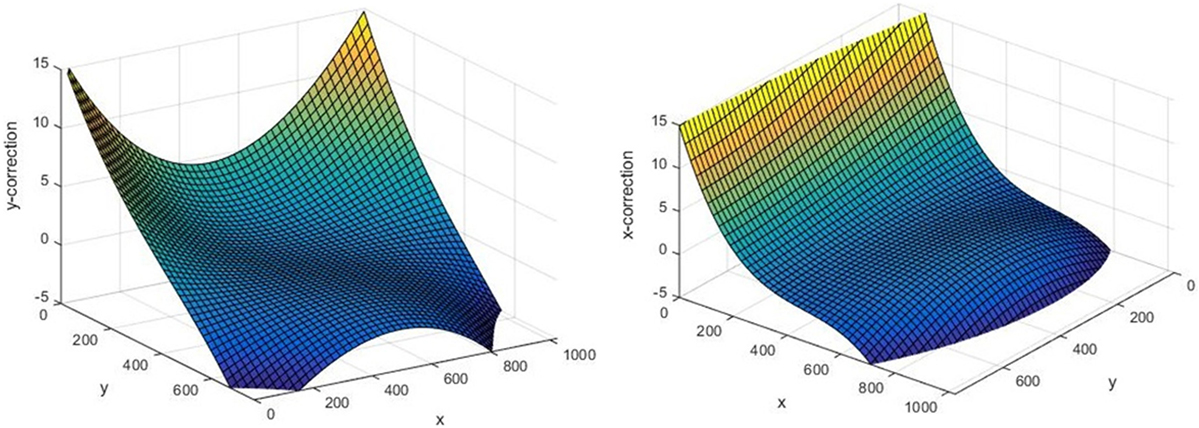
Figure 4. An example of resulting 3D polynomials for x and y corrections due to lens distortion. All units are in pixels.

Calibration maps of pixel sizes in centimeters in x and y directions are obtained using the same calibration pattern as lens distortion correction. Since the laser ensures the actual distance between thermal markers is constant, computing pixel size is a matter of examining every pair of adjacent points. Therefore, marker spacing becomes one and only physical measurement necessary for the entire calibration procedure, and is accomplished by overlaying the calibration pattern on top of a floating object of a known size (e.g., a wooden meter stick). In the example shown here the distance between markers was 5.5 cm throughout the pattern. Figure 5 (left) shows an example of the calibration pattern after correction for lens distortion (blue dots), which was then used to obtain realization of pixel sizes in x and y directions throughout the image in the locations shown with red dots. Based on these realizations, the resulting pixel size calibration map is modeled by fitting two planes shown in Figure 5 (right). Note, angle α is another important output of this perspective computation, which is the slope of the line connecting the camera with each pixel on the water surface (α = 0 corresponds to a vertical line). It is determined as α = arccos (nx/ny), where nx and ny are pixels size variables in x and y directions. This angle calculated for each pixel of each camera is used later (see “Image processing algorithm”) to compute vertical displacement.

FIGURE 5

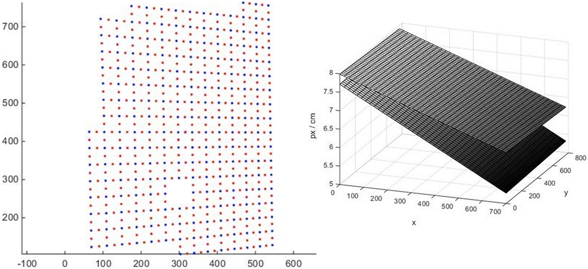
Figure 5. Left: blue dots show the calibration target markers corrected for lens distortion, thus all dots form straight lines. Red dots are locations of spacing realizations half way between markers. Right: pixel size maps, where upper plane is pixel size in the y direction, lower is in the x direction.

Once the physical location of calibration pattern markers is obtained for each camera, the final step of the calibration is collocation and alignment of their absolute horizontal location. If everything is done correctly, two images from two cameras will fit perfectly after a simple shift in x and y directions, see, for example, Figure 6. However, if polynomial fit errors were significant, some nonlinear misalignment might remain, which, if small, can be removed using additional offset correction, or, otherwise, will require a cleaner calibration procedure from the start.

FIGURE 6

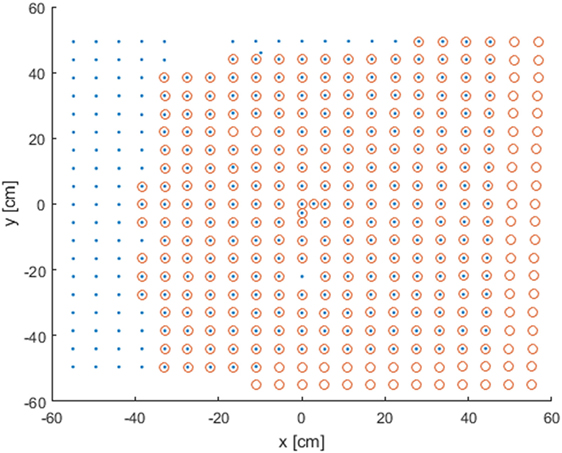
Figure 6. Calibration pattern after the completion of the calibration procedure obtained by both cameras (blue dots and red circles). Units correspond to centimeters along the flat water surface.

The Choice of a Thermal Pattern

The choice of the thermal pattern used to sample moving water surface involves a number of tradeoffs, which ultimately strongly depend on the application. Some of the parameters going into this consideration are: (1) Laser dwell time, or the time it takes for the laser beam to make a marker sufficiently bright to be detected by the IR cameras. (2) The minimal time the marker needs to remain visible with high enough signal to noise ratio. This parameter is a function of the laser dwell time, but also of the near-surface turbulence which acts to diffuse the marker. (3) Refresh rate, or the time intervals at which the thermal pattern should be refreshed. This parameter might be critical for applications requiring consequent time series analysis. (4) Spatial coverage, both in terms of smallest and largest scales to be resolved. (5) Directionality of the pattern, among others. The tradeoff often comes down to the choice between spatial and temporal scales to be resolved, and might be dependent on the intensity and other specifics of the flow measured in each particular case.

The regular grid pattern used for calibration (e.g., Figure 6) can be appropriate for some flow conditions and can be used with no changes, especially in cases with stronger flows. However, in weaker flow cases, it might result in some stereo collocation ambiguity due to the pattern self-similarity. To avoid this potential problem, a random number generator was used to generate x, y coordinate pairs. This makes every sub-region of the pattern unique and identifiable within the overall patter. However, a truly random distribution of points contains regions of undesirably high and low point densities, so, several iterations of Lloyd’s relaxation algorithm were applied to an otherwise random distribution of points. The resulting pattern used in this study is shown in Figure 7.

FIGURE 7

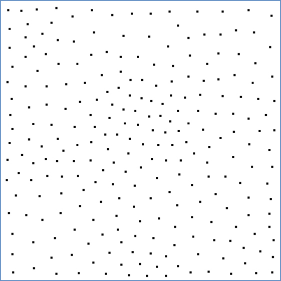
Figure 7. Random distribution of markers used as a sampling pattern in this study.

Image Processing Algorithm

The goal of the core image processing algorithm is to obtain x, y, and z locations of each marker at each time step. This information is then used to (1) reconstruct surface elevation maps at each time step and (2) to track these markers between consecutive frames to reconstruct surface velocity vector maps u, v, and w corresponding to all three spatial directions.

The algorithm starts by detecting markers in raw IR images. This is done by (1) masking out unwanted parts of the image, (2) adjusting contrast to remove background noise, (3) converting to black and white binary image, and (4) filtering out small speckles. The exact parameters used within these steps are setup specific and have to be adjusted accordingly.

Once an approximate location of a thermal marker is determined, the algorithm proceeds to resolve the mean location of the marker with subpixel resolution. This is done by an iterative scheme that assigns pixels weights according to their brightness and then looks for the center of mass of the entire marker with subpixel precision. The resulting precision of the marker center location estimate is approximately 1/20 of a pixel. At this point, the algorithm proceeds to use these high precision x (px) and y (px) locations of all detected markers and discards the rest of the image.

Various calibration and correction polynomial functions described in Section “Calibration” are applied directly to (x, y) marker coordinates. The result of this step is two sets of corrected physical space coordinates x (cm) and y (cm) of all markers detected by each of the two cameras.

The goal of the next step is to identify the same markers on both cameras. The technique used for this purpose is called “adaptive cross-correlation,” which is frequently used in particle image velocimetry systems (e.g., Scarano, 2001). First, a synthetic IR image is rendered by populating a dark frame with 2D Gaussian bell curves centered on each detected marker. This essentially recreates the original image minus all the noise, distortions, and need for calibration, e.g., Figure 8. Two synthetic images from two cameras are cross-correlated to find the most likely global shift (e.g., Figure 9, bottom-right). Then, two images are divided into quadrants with centers shifted using the global shift, such that the quadrant boundaries from one image match equivalent quadrants from another. This is done recursively to three levels deep (Figure 9), resulting in 8 × 8 sectors. Each sector provides a vector indicating how much this sector of the second image (i.e., image B) must be shifted to align with the equivalent sector of the first image (i.e., image A).

FIGURE 8

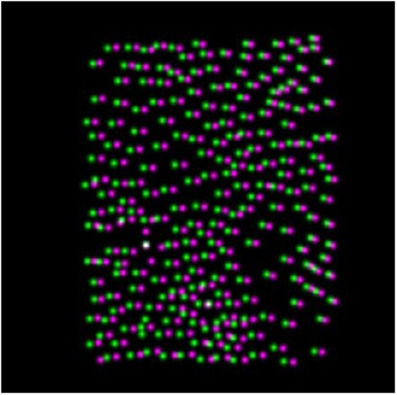
Figure 8. An example of two overlaid synthetic infrared images. Markers from different images are shown with different colors.

FIGURE 9

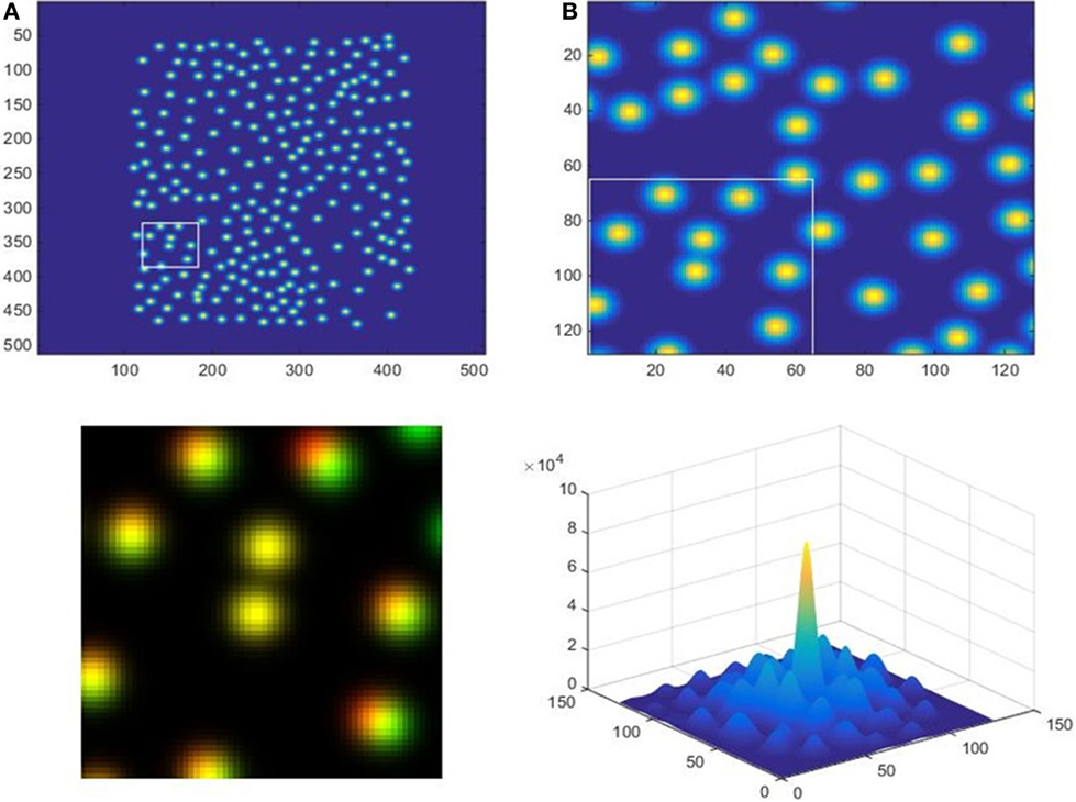
Figure 9. Upper left: the entire image (A), with a box around the current region being analyzed. Upper right: 1/16th of image (A), showing which of its quadrants (1/64th of the whole) is currently the focus. Lower left: blend of the two boxed regions, with red = image (A), green = image (B), and yellow = overlap. Lower right: cross-correlation of the two regions, with the peak giving the shift value.

The shifts obtained from the adaptive cross-correlation are applied to the second set of points, creating an adjusted copy which should be roughly aligned with the first set. This allows the assumption to be made that each point’s match is simply the nearest point to it in the other set, see Figure 9, bottom-left, as an example of shifted match for the smallest sub region. At this point, a maximum allowed displacement parameter can be chosen to filter out false points, but also allow for small roughness elements (if expected) to be resolved within the sub region. The result of this step is shown in Figure 10 with positive matches connected by lines. Only matched pairs are carried over to the next step.

FIGURE 10

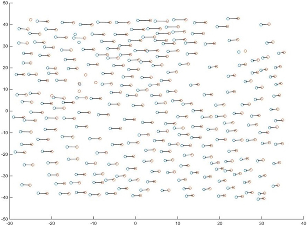
Figure 10. Detected markers on both cameras (blue and red circles) are shown in x (cm) and y (cm) coordinates, per calibration. Matches found on both images of an image pair are connected by lines. The rest are considered false points and are discarded.

The next step is to compute vertical coordinate z of each marker. The horizontal displacement Δx is attributed to the vertical deviation of the marker from the mean water level used during calibration. Then, the point’s height is calculated using the formula z = Δx/(tan α₁ + tan α₂), where α₁ and α₂ are the incidence angles corresponding to each pixel defined for each camera (see Calibration). The value of x assigned to this new 3D point is between the two original points, weighted by (tan α1)/(tan α1 + tan α2). The new y-component is simply the mean of the two markers’ y components.

The procedure to compute velocities from consecutive image pairs is remarkably similar to the one used to find matches within one image pair, except instead of matching between two images taken at the same time by different cameras, we compare two images taken by the same camera at different times. Once same markers are identified, the velocity is just the difference in their 3D positions divided by the time interval between the frames.

Results

The result is an array of marker locations with x, y, and z coordinates resolved for every frame pair and their u, v, and w velocities resolved between each consecutive pair of frames. For visualization purposes, in Figure 11, a 3D surface is fitted through x, y, and z coordinates of all points available from one image pair. The surface shows two crests and a trough of a random wave field. The mean surface is approximately 3 cm below 0, indicating some loss of water level since the calibration was done, probably due to evaporation.

FIGURE 11

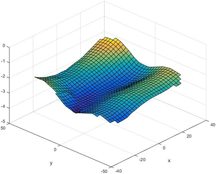
Figure 11. An example of resolved 3D water surface shape. All units are in centimeters. Color added for redundancy to visualize vertical displacement.

Horizontal projections of corresponding surface velocity vectors are shown for each marker in Figure 12. Velocity vectors corresponding to two wave crests appear to be moving mostly toward each other, indicating that one of the waves is a reflection from the end of the wave tank propagating back toward the wave generator (see Figure 1). There also appears to be a converging front collocated with one of the crests along y = −30. Note, the flow features resolved here are largely random and do not bear any significance other than to demonstrate the capability of STMV. Likewise, this study makes no attempt to validate these flow measurements, leaving the collection of a more rigorous validation dataset for future studies. The design of a validation experiment is expected to be a challenge in itself due to the lack of other means to collect comparable measurements. Meanwhile, a detailed discussion of potential sources of error is provided below.

FIGURE 12

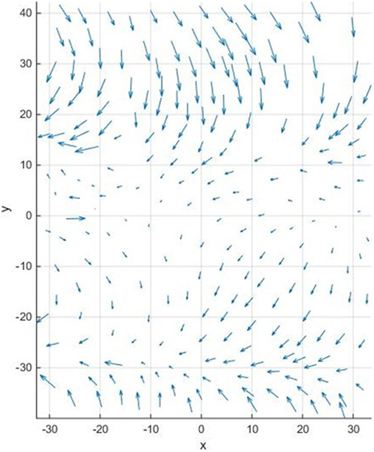
Figure 12. An example of horizontal u and v components of full 3D surface velocity vectors obtained for each thermal marker.

Discussion

The accuracy of the resulting measurements is a strong side of STMV. The precision of thermal marker’s center location estimate in decimal pixels is a function of number of pixels the marker occupies. Here, the average diameter was approximately six pixels, resulting in ~1/20 subpixel precision. In physical space, the accuracy is also a function of pixel size on the water surface, hence, it is a function of lens choice and a subject of tradeoff between higher accuracy and wider image footprint. Here, the pixel size varied around ~2.5 mm/px, depending on perspective and on the camera. This results in location precision of ~0.1 mm. The projection of each camera’s incidence angle has to be taken into account to calculate errors in x, y, and z directions. Generally, these errors will be of the same order, unless incidence angles of both cameras are too close to nadir, in which case, the error in z direction might increase significantly. Further, the velocity error is inversely proportional to time between frames, in this case, 0.1 mm × 30 Hz = 3 mm/s, already a remarkably low error value for a velocimeter. This error is absolute and is independent of the flow velocity. If measured flow is slow and lower error is desired, 30 Hz frame rate is likely unnecessary, hence it can be simply reduced, resulting in a proportional improvement in accuracy. Alternatively, a stronger lens or a higher resolution camera can be chosen to reduce pixel size. Spatial resolution and precision is another area of accuracy tradeoff. It is primarily a function of the thermal pattern choice, discussed in Section “The Choice of a Thermal Pattern.” Generally, a more powerful laser capable of generating more thermal markers per second paired with a more sensitive and higher resolution camera will result in a reduction of error and better temporal and spatial accuracy. Finally, although this method can be considered non-intrusive, it is possible to introduce enough heat into the FOV, so that the resulting buoyant currents will become comparable to the ambient flow field. This is particularly true in case a high refresh rate is desired for the thermal pattern in order to resolve time scales in the inertial subrange, yet, the mean flow is unable to advect old markers away. At some point, multiple overlaying markers will make Richardson number no longer negligible, which would imply that buoyancy effects are starting to influence shear produced turbulence, rendering the entire STMV method intrusive.

In a repeatable laboratory environment, STMV has another advantage, which is a possibility of synchronization with other components of the experiment, for example surface wave generator or towing carriage. This enables focusing on and studying specific features of the flow. The thermal pattern shape, location, and timing can be fine-tuned to densely seed highly intermittent phenomena, such as near wake behind a towed body, or a crest of a breaking wave, etc. Additionally, it is expected to be able to work with many other non-water surfaces (liquid or solid) just as effectively.

In the field, a significant care must be taken in order to remove platform motion, which will be effectively added to the flow velocities measured by STMV. A synchronized GPS/IMU unit collocated with cameras can resolve low frequency motions with sufficient accuracy and can then be used to correct STMV output. High frequency camera vibrations should be avoided as much as possible, but if present a correction algorithm can be potentially developed based on the application of a low pass filter to the raw imagery data cube. A significant advantage of STMV over single camera TMV is that it no longer requires synchronized water surface altimetry, as it is resolved inherently with the stereo approach. Also, if a particular application is only interested in relative flow motions within the FOV (i.e., vorticity, divergence, high wave number TKE spectra, etc.), mean velocity can be removed from each realization. In this case, platform motions no longer matter, making STMV system fully self-sufficient. Note, during the preparation of this paper, an STMV system successfully went through its first field trial onboard of R/P FLIP. Data obtained during this trial will be processed using the methodology described here and published in a follow-on paper.

Finally, an important discussion topic is the impact that the elevation of STMV above the water surface has on its performance. In the present configuration in the lab it was mounted at 2 m height, and preliminary FLIP data QC suggests it worked nearly equally well mounted 9 m above the ocean surface. However, as the elevation increases, the performance is expected to degrade. First, if the horizontal separation between two cameras is not increased proportionally, it will lead to rapid uncertainty increase in z coordinate and hence w velocity. Second, if cameras’ angle of view is held constant, the laser power will have to be increased proportionally to the physical area of the scene. Otherwise, a telescopic lens has to be used to keep the area of view unchanged. The laser beam divergence (2 mrads); however, cannot be reduced, making unavoidable thermal marker diameter increase a more fundamental limitation capping maximum STMV elevation. It is expected, however, that, in present configuration, it is possible to make thermal markers detectable with STMV positioned as high as 30 m above the surface, making lowest level airborne applications a possibility. In this case, thermal marker smearing due to the fast aircraft motion can be compensated for by programming the marking head to draw lines opposite but otherwise equal to the velocity of the aircraft.

Author Contributions

IS wrote the article, developed the idea and the hardware behind the described system, and executed experiments. JF developed calibration and image processing software.

Conflict of Interest Statement

The authors declare that the research was conducted in the absence of any commercial or financial relationships that could be construed as a potential conflict of interest.

The handling editor declared a shared affiliation, though no other collaboration, with one of the authors, IS.

Funding

Funding for this research was provided by ONR-NRL program element 61153N, WU BE023-01-41-1C04.

References

Garbe, C. S., Schimpf, U., and Jähne, B. (2004). A surface renewal model to analyze infrared image sequences of the ocean surface for the study of air-sea heat and gas exchange. J. Geophys. Res. Oceans 109. doi: 10.1029/2003JC001802

CrossRef Full Text | Google Scholar

Handler, R. A., Savelyev, I., and Lindsey, M. (2012). Infrared imagery of streak formation in a breaking wave. Phys. Fluids 24, 121701. doi:10.1063/1.4769459

CrossRef Full Text | Google Scholar

Handler, R. A., and Smith, G. B. (2011). Statistics of the temperature and its derivatives at the surface of a wind-driven air-water interface. J. Geophys. Res. Oceans 116. doi:10.1029/2010JC006496

CrossRef Full Text | Google Scholar

Handler, R. A., Smith, G. B., and Leighton, R. I. (2001). The thermal structure of an air-water interface at low wind speeds. Tellus 53, 233–244. doi:10.3402/tellusa.v53i2.12187

CrossRef Full Text | Google Scholar

Haußecker, H., Schimpf, U., and Jahne, B. (1998). “Measurements of the air-sea gas transfer and its mechanisms by active and passive thermography,” in IEEE International Geoscience and Remote Sensing Symposium Proceedings, IGARSS’98, Vol. 1 (Seattle, WA), 484–486.

Google Scholar

Jähne, B., Libner, P., Fischer, R., Billen, T., and Plate, E. J. (1989). Investigating the transfer processes across the free aqueous viscous boundary layer by the controlled flux method. Tellus B Chem. Phys. Meteorol. 41, 177–195. doi:10.1111/j.1600-0889.1989.tb00135.x

CrossRef Full Text | Google Scholar

Marmorino, G., Savelyev, I., and Smith, G. B. (2015). Surface thermal structure in a shallow-water, vertical discharge from a coastal power plant. Environ. Fluid Mech. 15, 207–229. doi:10.1007/s10652-014-9373-0

CrossRef Full Text | Google Scholar

Marmorino, G. O., and Smith, G. B. (2007). Infrared imagery of a turbulent intrusion in a stratified environment. Estuaries Coasts 30, 671–678. doi:10.1007/BF02841964

CrossRef Full Text | Google Scholar

Marmorino, G. O., Smith, G. B., and Lindemann, G. J. (2004). Infrared imagery of ocean internal waves. Geophys. Res. Lett. 31. doi:10.1029/2004GL020152

CrossRef Full Text | Google Scholar

Marmorino, G. O., Smith, G. B., and Lindemann, G. J. (2005). Infrared imagery of large-aspect-ratio Langmuir circulation. Cont. Shelf Res. 25, 1–6. doi:10.1016/j.csr.2004.08.002

CrossRef Full Text | Google Scholar

Marmorino, G. O., Smith, G. B., Miller, W. D., and Bowles, J. H. (2010). Detection of a buoyant coastal wastewater discharge using airborne hyperspectral and infrared imagery. J. Appl. Remote Sens. 4, 043502–043502. doi:10.1117/1.3302630

CrossRef Full Text | Google Scholar

Marmorino, G. O., Smith, G. B., Toporkov, J. V., Sletten, M. A., Perkovic, D., and Frasier, S. J. (2009). Airborne imagery of ocean mixed-layer convective patterns. Deep Sea Res. I Oceanogr. Res. Pap. 56, 435–441. doi:10.1016/j.dsr.2008.10.007

CrossRef Full Text | Google Scholar

Melville, W. K., Shear, R., and Veron, F. (1998). Laboratory measurements of the generation and evolution of Langmuir circulations. J. Fluid Mech. 364, 31–58. doi:10.1017/S0022112098001098

CrossRef Full Text | Google Scholar

Savelyev, I., Thomas, L. N., Smith, G. B., Wang, Q., Shearman, R. K., Haack, T., et al. (2018). Aerial observations of symmetric instability at the north wall of the Gulf Stream. Geophys. Res. Lett. 45, 236–244. doi:10.1002/2017GL075735

CrossRef Full Text | Google Scholar

Savelyev, I. B., Maxeiner, E., and Chalikov, D. (2012). Turbulence production by nonbreaking waves: laboratory and numerical simulations. J. Geophys. Res. Oceans 117. doi:10.1029/2012JC007928

CrossRef Full Text | Google Scholar

Scarano, F. (2001). Iterative image deformation methods in PIV. Meas. Sci. Technol. 13, R1. doi:10.1088/0957-0233/13/1/201

CrossRef Full Text | Google Scholar

Sutherland, P. (2013). On Breaking Waves and Turbulence at the Air-Sea Interface. Ph.D. thesis, University of California, San Diego.

Google Scholar

Sutherland, P., and Melville, W. K. (2013). Field measurements and scaling of ocean surface wave-breaking statistics. Geophys. Res. Lett. 40, 3074–3079. doi:10.1002/grl.50584

CrossRef Full Text | Google Scholar

Sutherland, P., and Melville, W. K. (2015a). Measuring turbulent kinetic energy dissipation at a wavy sea surface. J. Atmos. Oceanic Technol. 32, 1498–1514. doi:10.1175/JTECH-D-14-00227.1

CrossRef Full Text | Google Scholar

Sutherland, P., and Melville, W. K. (2015b). Field measurements of surface and near-surface turbulence in the presence of breaking waves. J. Phys. Oceanogr. 45, 943–965. doi:10.1175/JPO-D-14-0133.1

CrossRef Full Text | Google Scholar

Veron, F., and Melville, W. (2001). Experiments on the stability and transition of wind-driven water surfaces. J. Fluid Mech. 446, 25–65. doi:10.1017/S0022112001005638

CrossRef Full Text | Google Scholar

Veron, F., Melville, W., and Lenain, L. (2008). Infrared techniques for measuring ocean surface processes. J. Atmos. Oceanic Technol. 25, 307–326. doi:10.1175/2007JTECHO524.1

CrossRef Full Text | Google Scholar

Veron, F., Melville, W., and Lenain, L. (2009). Measurements of ocean surface turbulence and wave-turbulence interactions. J. Phys. Oceanogr. 39, 2310–2323. doi:10.1175/2009JPO4019.1

CrossRef Full Text | Google Scholar

Zhang, X., and Harrison, S. (2004). A laboratory observation of the surface temperature and velocity distributions on a wavy and windy air-water interface. Phys. Fluids 16, L5–L8. doi:10.1063/1.1631813

CrossRef Full Text | Google Scholar