Numerical Solution of the Radiation Transport Equation at an Air-Water Interface for a Stratified Medium

Introduction

The goal of determining the physical mechanisms responsible for the transport of mass, momentum and energy across the air-sea interface has driven research in recent years since such knowledge may, among other things, contribute to more accurate estimates for the evolution of the climate of the earth. Although bulk parameterization provides estimates of the net transport of heat and gases, their transport is ultimately controlled by thin temperature and concentration boundary layers that form at the air-sea boundary (Fairall et al., 1996). In recent years, however, significant efforts have succeeded in uncovering the microphysics controlling thermal and gas fluxes by employing controlled laboratory experiments (Katsaros et al., 1977; Jahne et al., 1987; Handler et al., 2001; Handler and Smith, 2011).

More specifically, atmospheric accumulation of greenhouse gases such as CO₂, has attracted great attention in recent decades. The rate at which such gases are taken up by the oceans continue to remain somewhat uncertain despite significant recent research (Wanninkhof, 1992, 2014). The determination of these gas fluxes is a difficult task, but in recent decades, it was pointed out that gas flux could be estimated from heat flux measurements (Atmane et al., 2004). This can be achieved by measuring the heat flux, and using the ratio of gas Schmidt number to the Prandtl number to estimate gas flux. If such an analogy between heat and gas flux is valid, then remote infrared (IR) measurements of the ocean surface could be used to extract heat flux and then converted to gas flux. In addition, such a method would allow large regions of the ocean to be mapped by aircraft or satellite, giving unprecedented maps of oceanic gas flux. In addition, heat flux is obviously an important quantity, in and of itself.

Direct measurement of the temperature profile at an air-water interface using probes such as thermocouples and fast response thermistors is difficult owing to the extremely small thickness of these thermal layers, typically from 0.1 to 1 mm. The temperature difference across these layers, often referred to as the cool-skin, can be as large as T = 1.0 K (Katsaros et al., 1977). However, recent advances in remote sensing hardware, in particular infrared (IR) imagers, have stimulated the development of unique approaches to extracting heat fluxes from image based techniques (Garbe et al., 2004). Numerical simulations have also provided insight into the small-scale turbulent dynamics that determine these fluxes (Handler et al., 1999; Leighton et al., 2003; Nagaosa and Handler, 2003, 2012; Handler and Zhang, 2013; Herlina and Wissink, 2014; Fredriksson et al., 2016a,b). We point out here that the very thin thermal boundary layer at the air-sea interface is formed as a result of a competition between upward heat flux out of the interface, which tends to increase the thermal layer thickness, and subsurface turbulence, which tends to decrease it as a result of the surface renewal of bulk fluid. The detailed physics of this is well-known, and is well-described elsewhere (Jahne et al., 1989; Handler et al., 1999, 2001; Atmane et al., 2004; Handler and Zhang, 2013).

Past and recent efforts have used both aircraft and satellite platforms equipped with radiometers and/or thermal imagers to produce sea-surface temperature products in addition to attempts to determine oceanic heat flux. As heat flux may serve as a proxy for gas flux (Jahne et al., 1987), having a robust instrument and atmospheric sounding retrieval technique could provide wide area maps of simultaneously acquired heat and gas transport. Early efforts for remotely extracting heat flux by McAlister and McLeish (1970) and McAlister et al. (1971) exploit the varying optical depth of thermal radiation within the aqueous layer in wavelength bands that are transparent to the atmosphere (Downing and Williams, 1975). This approach was revisited some 30 years later by McKeown et al. (1995) and McKeown and Leighton (1999), who performed laboratory experiments using band-pass filters and an imaging array.

Consistent with the goals stated above, and as discussed in Handler and Judd (2018), our motivation is to accurately estimate the magnitude and direction of the radiation emerging from a thermally stratified medium. In that work, the problem was made tractable by employing simplifying assumptions (e.g., ignoring surface waves, scattering, assuming a linear temperature profile, and taking only the first term in a series expansion of the Planck spectrum). This allowed the governing radiation transport equation to be solved exactly. The result provides the deviation of the surface radiation intensity from the Planck spectrum in terms of three non-dimensional numbers. However, thermal profiles are found to have a non-linear character, typically varying as a decaying exponential over the boundary layer thickness. To elucidate the nature of this non-linear stratification, in the present work we remove the previously employed linearity assumptions, and estimate the surface radiation for several more realistic thermal profiles (Smith et al., 2001). This requires the numerical integration of the transport equation. Results are obtained for both a constant temperature surface boundary condition, and the more frequently encountered constant heat flux condition.

Radiation Transport Equation in a Stratified Medium

The details of the development of the governing equation and its solution can be found in Handler and Judd (2018); however, for completeness we briefly define the problem. The radiation transport equation (RTE) for an emitting and absorbing medium takes the form (Chandrasekhar, 1960):

$\frac{dI}{ds}=-k\text{ρ}I+\text{ρ}j\begin{array}{cc}& (1)\end{array}$

where I is the radiation intensity, s is the coordinate associated with a spatial direction, k is the opacity, ρ is the density of the medium, and j is the emission coefficient. From local thermodynamic equilibrium j takes the form:

$j=kB\left(T,\text{λ}\right)\begin{array}{cc}& (2)\end{array}$

where B(T,λ) is the Planck spectrum and is given by:

$B\left(T,\text{λ}\right)=\frac{C_1}{{\lambda }^5}\left[\frac{1}{e^{\left(C_2(\text{λ})/T\right)}-1}\right]\begin{array}{cc}& (3)\end{array}$

The radiation constants take the form, C₁ = 2hc², C₂(λ) = hc/λk_b, h is Planck's constant, c is the speed of light, λ is the wavelength of radiation, k_b is the Boltzmann's constant, and T is the absolute temperature. Figure 1 shows the geometry considered for the radiation field in a stratified medium, which represents an aqueous layer bounded above by an air mass. The temperature in the aqueous layer is assumed to be stratified in planes parallel to the air-water interface defined at y = 0.

FIGURE 1

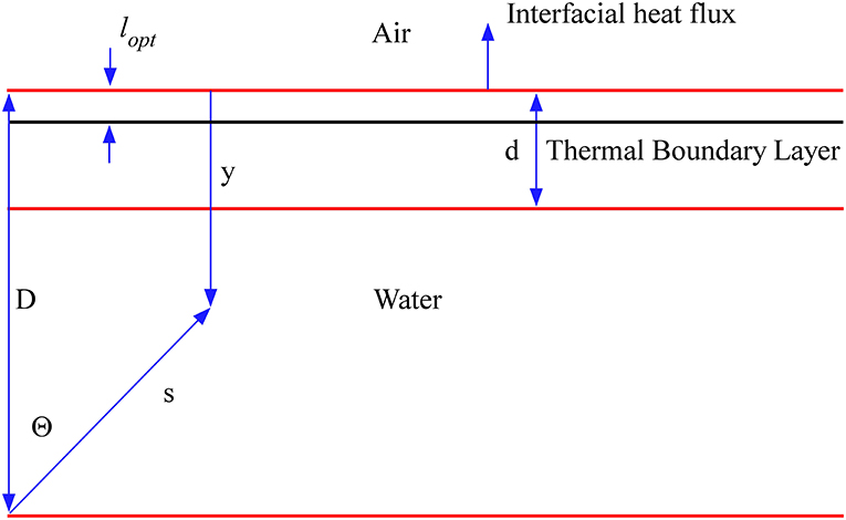
Figure 1. Schematic of geometry and radiation field at an air-water interface.

As shown in Figure 1, three length scales are of importance: (1) The thermal layer thickness d, (2) An outer scale D, and (3) the optical depth, l_opt, of the medium. For future reference, we define a linearly varying temperature field (Handler and Judd, 2018) given by:

$T\left(y\right)=\{\begin{array}{c}\frac{\Delta T}{d}y+T_0,0\le y<d\\ T_d,d\le y<D& (4)\end{array}$

where ΔT = T_d − T₀, T₀ = T(0) is the temperature at the air-water interface, and T_d = T(d). The coordinate y can be related to s giving y = D − scos(θ). Inserting this into Equation (1), and integrating yields:

$I\left(y\right)=I_D{e}^{\frac{\beta (\text{λ})}{\cos \theta }(y-D)}+\frac{\beta (\text{λ})}{\cos \theta }{\displaystyle {\int }_y^{D}B(T,\text{λ})e^{\frac{\beta (\text{λ})}{\cos \theta }(y-\overline{y})}d\overline{y,}\begin{array}{cc}& (5)\end{array}}$

where I_D and is the radiation intensity at y = D.

Numerical Solution of the RTE in a Stratified Medium with a Linear Temperature Profile

As previously noted, no known closed form solution exists for the general integral equation, Equation (5), for the given temperature profile, Equation (4). Here solutions to this expression will be obtained using a numerical approach. These will then be compared to the approximate solution developed for small temperature perturbations. In Equation (5) the term $\beta (\lambda )=\frac{1}{l_{opt}(\lambda )}$ is the reciprocal of the wavelength dependent optical depth. In this work, we examine radiation in two commonly defined thermal wavelength bands: the 3–5 μm (mid-wave or MWIR) and the 8–14 μm (long-wave or LWIR) bands. The optical depth is rather shallow for both bands, varying from 1 to 90 microns in the MWIR band and 3–19 microns in the LWIR band (Downing and Williams, 1975). In these calculations, we will use an aqueous thermal boundary layer thickness of d = 1 mm, and outer layer of D = 0.5 m, and a surface temperature T(y = 0) = T₀ = 300 K.

The radiation intensity at the interface, y = 0, is as follows:

$I\left(0\right)=I_D{e}^{\frac{\beta (\text{λ})}{\cos \theta }(-D)}+\frac{\beta (\text{λ})}{\cos \theta }{\displaystyle {\int }_0^{D}B(T,\text{λ})e^{\frac{\beta (\text{λ})}{\cos \theta }(-y)}dy.\begin{array}{cc}& (6)\end{array}}$

For our purposes, we consider radiation in a direction perpendicular to the interface (θ = 0) such that the signal is maximal (Zel'dovich and Raizer, 1966). With the assumption that the water depth is effectively infinite ($\frac{D}{d}\gg 1$), and that $\frac{D}{l_{opt}}⋙1$, we obtain:

$I\left(0;\text{λ}\right)=\beta \left(\text{λ}\right){\displaystyle {\int }_0^{D}B\left(T\left(\overline{y}\right),\text{λ}\right)e^{\beta \left(\text{λ}\right)\left(-y\right)}d\overline{y.}\begin{array}{cc}& (7)\end{array}}$

For clarity, the dependence of the radiation intensity on wavelength, and the Planck spectrum on temperature has been indicated. We initially addressed Equation (7) numerically using an in-house written composite Simpson's 3/8 rule integration scheme thus permitting greater flexibility in controlling the governing input parameters compared to a commercial computational package. The thermal stratification in these computations is linear as defined in Equation (4), so as to compare with theory (Handler and Judd, 2018):

$\begin{array}{cc}\frac{I\left(0\right)-B(T_0)}{B(T_0)}=K_1{K}_2{K}_3\text{ cos }\theta & (8)\end{array}$

$\begin{array}{r}where{K}_1=\frac{C_2}{T_0},K_2=\frac{\Delta T}{T_0},and{K}_3=\frac{l_{opt}}{d}.\end{array}$

We define the relative signal strength as $\overline{I}where\overline{I}=\left[I(0)-B(T_0)\right]/B(T_0)$. Figure 2A shows the comparison of theory and computation for the excess of surface radiation intensity with respect to the Planck spectrum in the 3–5 micron waveband. As in Handler and Judd (2018) we will refer to this quantity as the signal. The numerical results agree well over the band with exception of the range λ ≲ 3.15 μm, the blue rectangle in the figure. Figure 2B is an exploded view of this region where the numerical result deviates as it approaches the lower bound of the mid-wave band. We speculate that this behavior is related to the very small optical depth (l_opt(λ) < 3μm) over this wavelength range, resulting in difficulty in resolving the region with uniform grid spacing. An increase in the number of node points in the computational scheme lessened the deviation from the theory, but did not completely remove the effect. To fully resolve this region we employed an adaptive scheme (Gauss-Kronrod quadrature) from MATLAB R2016a (MathWorks Inc., Natick, MA, USA). Application of the adaptive scheme and results are discussed in the next section where more realistic thermal boundary layer profiles are considered. The same composite Simpson's rule was applied to the long-wave range in Figure 3. The resulting theoretical and numerical curves compare favorably over the entire waveband. This is likely in part due to the fact that unlike the optical depths for mid-wave radiation which decrease below 3 μm, long-wave optical depths are l_opt(λ) ≥ 3μm over the entire waveband.

FIGURE 2

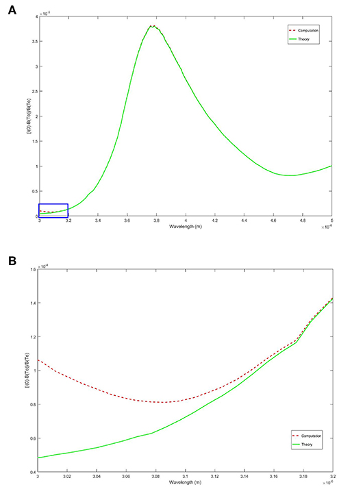
Figure 2. The top figure, (A), is a plot of the numerical and theoretical approximations over the entire MWIR band. The results compare favorably over the entire range with exception of the lower bound of the interval. (B) is a magnified view of the curves in the blue rectangle of (A). Below 3.15 micron the numerical solution begins to slowly diverge and eventually deviates from theory at 3 micron by 119%.

FIGURE 3

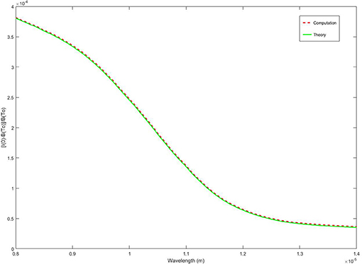
Figure 3. Comparison of numerical result to theoretical approximation over the entire long-wave band.

Finally, we address the behavior of the theoretical and numerical results as a function of the temperature difference, ΔT = T_d − T₀, across the thermal layer. The temperature was varied over the range of values given by ΔT = 0.1 K, 0.5 K, 1.0 K, with all other variables fixed as previously stated. It is evident from Figure 4 (and Equation 8) that the theoretical signal decreases with decreasing temperature difference.

FIGURE 4

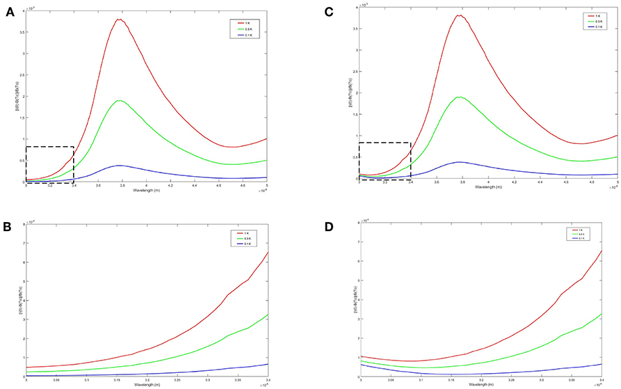
Figure 4. Behavior of the theoretical approximation (A,B), and the numerical results (C,D), as a function of the temperature difference ΔT = T_d − T₀ across the thermal layer for a linear temperature profile. (B,D) are magnified views of the dashed rectangles in (A,C) respectively. In both the plots of the theoretical and numerical results, it is evident that the signal decreases as the temperature difference across the thermal layer decreases.

Although we have not presented the results for the long-wave band, a similar decrease in signal strength was observed for both the theoretical and computational results as the temperature difference was decreased.

Non-linear Stratification

The theoretical and computational results for the linear profile validates the approach used here, so that it can now be employed to determine the surface radiation resulting from more realistic thermally stratified layers. Here we consider two surface conditions; a constant surface temperature and the more frequently encountered constant surface heat flux condition (Csanady, 2001). Several temperature distributions, including the linear profile in Equation (4) are examined.

The thermal boundary layers for the constant temperature surface condition are listed in Equations (9a-d). The definition of the symbol i used in 9c and 10d is provided in Appendix, additional details can be found in Gautschi (1961).

$T\left(y\right)=\{\begin{array}{c}\left(\frac{\Delta T}{d}\right)\left[2y-\frac{y^2}{d}\right]+T_0,0\le y\le d(a)\\ \left(\frac{\Delta T}{2d}\right)\left[3y-\frac{y^3}{d^2}\right]+T_0,0\le y\le d(b)\\ -\Delta T4i^{2}erfc\left(\frac{\sqrt{\pi }}{4\delta }y\right)+T_d,0\le y\le d(c)\\ T_d,d\le y\le D(d)& (9)\end{array}$

In Figure 5 each of these thermal profiles [Equations (4, 9a–c)] are determined with T(y = 0) = T₀ = 300 K and T(y = d) = T_d = 301 K where d = 1 × 10⁻³ m is the edge of the thermal layer. Equations (9a,b) are standard polynomial approximations (Kays and Crawford, 1993). The temperature distribution in equation (9c) incorporates a surface renewal model (Liu and Businger, 1975; Katsaros et al., 1977), adapted for a constant surface temperature boundary condition. We note that for fixed temperature boundary conditions, the slope for each of the profiles at and near the surface (y = 0) varies from curve-to-curve as shown in Figures 5, 6. This hierarchy of thermal stratification becomes important when comparing the results of the signal strength and will be discussed in the next section.

FIGURE 5

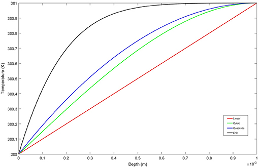
Figure 5. Model temperature distributions (thermal stratification) for constant surface temperature condition T₀ = 300 K and T_d = 301 K at the edge of the thermal boundary layer at a depth of y = 1 × 10⁻³ m. The curves blend into a constant temperature profile at y = 1 × 10⁻³ m that extends to the domain depth at y = 0.5 m. The parameter δ in Equation (9c) was adjusted so that the absolute error of T(y = 1 × 10⁻³ m) and T_d = 301 K was made <1 × 10⁻⁴ K.

FIGURE 6

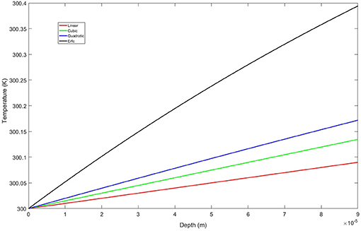
Figure 6. Structure of thermal boundary layers for fixed surface temperature over the optical depths of both the mid- and long-wave thermal bands.

We also consider thermal profiles corresponding to a constant surface flux, $\frac{dT(y=0)}{dy}=constant,$with $q=k\frac{\Delta T}{d}=608W{m}^{-2}$ which is approximately the heat flux obtain in the experiments by Handler and Smith (2011) for a wind speed of 3 ms⁻¹. These temperature profiles are given by:

$T\left(y\right)=\{\begin{array}{c}\left(\frac{\Delta T}{d}\right)\left[y-\frac{y^2}{2d}\right]+T_0,0\le y\le d(a)\\ \left(\frac{\Delta T}{d}\right)\left[y-\frac{y^3}{3d^2}\right]+T_0,0\le y\le d(b)\\ -\Delta Texp\left(\frac{-y}{\delta }\right)+T_d,0\le y\le d\left(c\right)\\ -\Delta T6i^{3}erfc\left(\frac{2}{3\sqrt{\pi }\delta }y\right)+T_d,0\le y\le d\left(d\right)\\ T_d,d\le y\le D(e)& (10)\end{array}$

The exponential and Erfc curves in Figure 7A asymptote to T_d = 301 K with the domain depth set at y = 9.25 × 10⁻³ m, which is the location where the exponential curve attains 99.99% of T_d. For the cubic and quadratic models, the edge of the thermal boundary layer is treated as if it occurs at y = 1 x 10⁻³ m, with the cubic reaching T = 300.667 K and the quadratic T = 300.500 K. Figure 7B shows that the linear temperature distribution has the largest net change in temperature over the thermal boundary layer and bounds the profiles. Upon closer examination of the very near-surface region shown in Figure 8, we see that all the profiles are nearly linear, with the linear profile slightly higher than all the others.

FIGURE 7

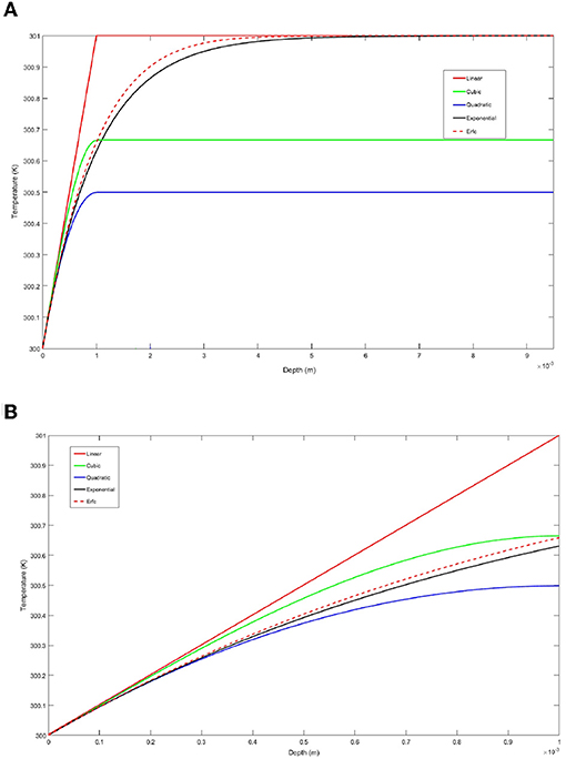
Figure 7. Model temperature distributions (thermal stratification) for constant surface heat flux condition with $q=k\frac{\Delta T}{d}=608W{m}^{-2}$. All of the curves have the same slope, ΔT/d, at y = 0. The exponential and Erfc curves in (A) asymptote to T_d = 301 K with the domain of the depth set at y = 9.25 × 10⁻³ m which is the location where the exponential curve attains 99.99% of T_d. For the cubic and quadratic models, the edge of the thermal boundary layer is treated as if it occurs at y = 1 × 10⁻³ m, with the cubic reaching T = 300.667 K and the quadratic T = 300.500 K. (B) is an exploded view of the thermal boundary layer, left hand side of (A).

FIGURE 8

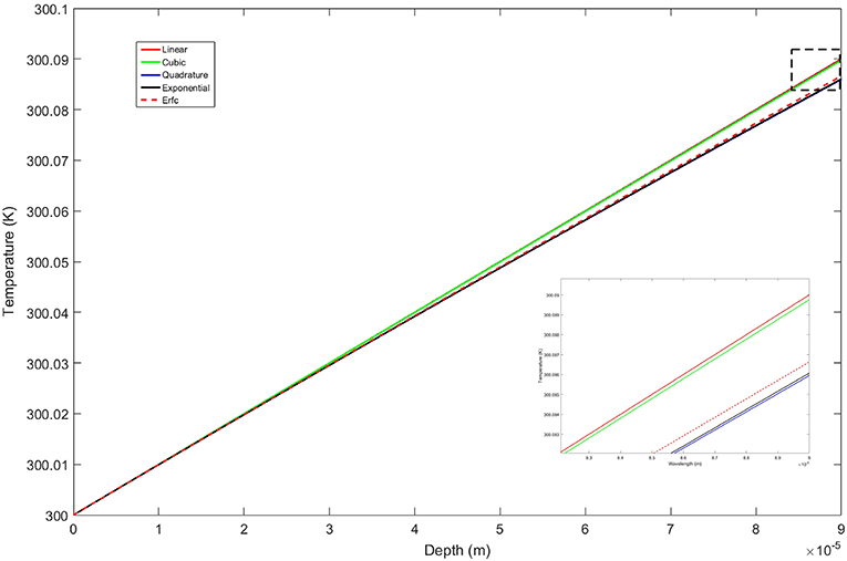
Figure 8. Structure of the thermal boundary layers for fixed heat flux extending over the optical depths for both the mid- and long-wave thermal bands. The inset is of the dashed rectangle in the upper right of the curve and shows the hierarchy of the temperature profiles.

Results for Non-linear Stratification

To determine the surface radiation intensity, the above temperature profiles were substituted into Equation (7), and the MATLAB Integral function was used to perform the integration. This is a global adaptive quadrature routine with the relative and absolute tolerances set to 10⁻⁸ and 10⁻¹², respectively. Figure 9A shows the signal for the constant temperature boundary condition with a fixed temperature change of ΔT = 1.0 K across the surface layer over the mid-wave band for the various profiles. Here we repeat the computation for the linear profile and compare it with the theoretical result (Figure 9B). It is evident that the curves match well over the entire range of wavelengths, even below λ ≲ 3.15 μm where large deviations from the theoretical values were previously observed (see Figure 2B). Most notably in Figure 9A, as the temperature profile becomes fuller, the resulting gradient is steeper and the signal tends to increase in magnitude. The hierarchy from smallest to largest overall signal as a function of temperature distribution is as follows; linear, cubic, quadratic, and Erfc with the peak of all the curves occurring at λ ≈ 3.8 μm. This is not unexpected as the optical depth is largest, ~90 × 10⁻⁶ m, at this location and drops off on either side of the peak. A similar behavior was observed in the signal curve for the long-wave band, Figure 10, with the peak occurring at the lower bound of the waveband at λ ≈ 8 μm, which is again where the optical depth attains its largest value ~19 × 10⁻⁶ m.

FIGURE 9

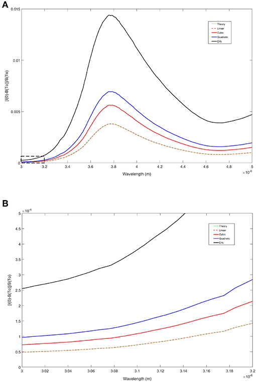
Figure 9. (A) Comparison of MWIR radiation emitted from an air-water surface made dimensionless with the Planck spectrum for several thermal stratifications for a constant surface temperature condition. The dashed box, lower left corner of graph, is the same region in Figure 2A. (B) is a magnified view of the dashed box and the numerical results for the linear profile show very good agreement with the theoretical result.

FIGURE 10

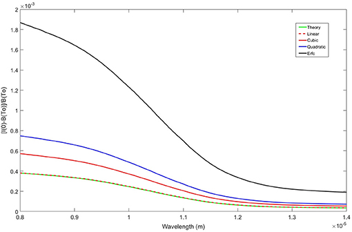
Figure 10. Comparison of LWIR radiation emitted from an air-water surface made dimensionless with the Planck spectrum for several thermal stratifications for a constant surface temperature condition. As with the mid-wave case, the numerical results for the linear profile show very good agreement with the theoretical result.

In general, an increase in the signal of the emitted surface radiation for both the mid-wave and long-wave bands is associated with the temperature profile that increases in magnitude the most over their respective optical depths. In the case of the constant surface temperature, Figure 5, the Erfc distribution dominates all other profiles with representative increases in temperature of ΔT = 0.4 K at a depth of 90 × 10⁻⁶ m and ΔT = 0.1 K at 19 × 10⁻⁶ m. For comparison the next largest profile is the quadratic with increases in temperature of ΔT = 0.17 K at a depth of 90 × 10⁻⁶ m and ΔT = 0.04 K at 19 × 10⁻⁶ m. The change in relative signal strength $\overline{I}$ at λ ≈ 3.8 μm, the wavelength with the largest optical depth in the mid-wave band, between the Erfc and quadratic profile is $\Delta \overline{I}={\overline{I}}_{Erfc}-{\overline{I}}_{Quad}=0.00745$, implying that the Erfc signal is almost double that of the quadratic. Likewise for the long-wave band at its maximum optical depth (λ ≈ 8 μm), $\Delta \overline{I}=0.001120$, implying that the Erfc signal is 2.5x that of the quadratic.

For the constant heat flux boundary condition, the relative changes in signal strength are less significant, and in fact the linear profile which resulted in the weakest signal for the constant temperature case now produces the strongest, Figures 11, 12. Upon closer examination of the temperature profiles, all of them are nearly linear over the optical depth layer for the mid- and long-wave bands (Figure 8). Representative changes in temperature of the linear profile, which provides an upper bound for the family of temperature distributions, are ΔT = 0.0899 K at a depth of 90 × 10⁻⁶ m and ΔT = 0.0189 K at 19 × 10⁻⁶ m. For purposes of comparison, we take a closer look at the temperature and signal variations between the linear profile and the quadratic model which provides a lower bound for the family of temperature distributions. The increase in temperature of the quadratic profile at 90 × 10⁻⁶ m is ΔT = 0.0859 K and ΔT = 0.0187 K at 19 × 10⁻⁶ m. The resulting change in relative signal strength at λ ≈ 3.8 μm is $\Delta \overline{I}={\overline{I}}_{Lin}-{\overline{I}}_{Quad}=3.460\times 10^{-4}$, implying that the linear signal is ~10% larger than the quadratic. For the long-wave band at λ ≈ 8 μm the change in signal is $\Delta \overline{I}=7.30\times 10^{-6}$ implying the linear signal is ~2% larger than the quadratic.

FIGURE 11

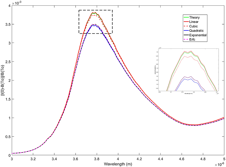
Figure 11. Comparison of MWIR radiation emitted from an air-water surface made dimensionless with the Planck spectrum for several thermal stratifications for a constant surface heat flux condition. The inset is a magnified view of the dashed rectangle surrounding the peak of the curves at λ ≈ 3.8 x 10⁻⁶ m.

FIGURE 12

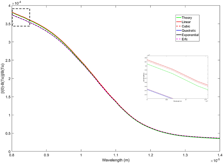
Figure 12. Comparison of LWIR radiation emitted from an air-water surface made dimensionless with the Planck spectrum for several thermal stratifications for a constant surface temperature condition. The inset is a magnified view of the dashed rectangle surrounding the curves at λ ≈ 8 x 10⁻⁶ m.

Summary and Conclusions

We have numerically addressed the problem of determining the radiation intensity or signal of thermal infrared radiation emitted from an air-water interface for a thermally stratified aqueous layer. Our effort is motivated by the possibility of determining, by solely passive means, the transport of heat and gas from the air-sea interface, a problem of importance in determining global climate evolution (Wanninkhof, 1992, 2014).

The approach taken was to numerically integrate the radiation transport equation with a linearly varying temperature field, validate the results with a previously derived analytical expression, and to go further by using a family of more realistic thermal boundary layer profiles. Results for both constant temperature and constant heat flux boundary conditions were obtained. In order to retain the non-linear features of the problem, few simplifications were imposed beyond making the assumption that the optical depth is small compared to the thermal boundary layer dimension, and that the depth of the domain is effectively infinite.

A main result for both surface boundary conditions is that the numerical analysis compares favorably with the linear thermal profile theoretical approximation for both the mid- and long-wave regimes. This more extensive analysis provides additional evidence that the previous theoretical model, approach, and attendant assumptions are reasonable and that Equation (8) provides insight to key parameters that control the signal strength.

However, it is important to note that the surface boundary condition and structure of the underlying thermal stratification may interact to control the signal strength. For a constant surface temperature state, representative signal strength varied as much as 200% for the mid-wave band and 250% for the long-wave region. We speculate that the source of the increase in signal strength may be traced directly to the structure of the thermal layer and its overlap with the optical depths for each waveband.

The more common physical state encountered at air-water interfaces is that of a constant heat flux. This condition fixes the structure of the thermal stratification and the thermal profiles to be nearly linear over the optical depth layer (see Figure 8) for both the mid- and long-wave band. That is, the influence due to thermal stratification may be considered a higher order effect. Compared to the constant surface temperature state, representative signal strengths experience much more modest variations, with the mid-wave band varying by 10% and the long-wave by 2%. We conclude that the theoretical approximation (Handler and Judd, 2018) can be used with confidence to accurately estimate the radiation from a stratified interface under realistic conditions.

Author Contributions

All authors listed have made a substantial, direct and intellectual contribution to the work, and approved it for publication.

Conflict of Interest Statement

The authors declare that the research was conducted in the absence of any commercial or financial relationships that could be construed as a potential conflict of interest.

References

Atmane, M. A., Asher, W. E., and Jessup, A. T. (2004). On the use of the active infrared technique to infer heat and gas transfer velocities at the air-water free surface. J. Geophys. Res. 109:C08S14. doi: 10.1029/2003JC001805

CrossRef Full Text | Google Scholar

Chandrasekhar, S. (1960). Radiative Transfer. New York, NY: Dover Publications.

Google Scholar

Csanady, G.T. (2001). Air-Sea Interaction: Laws and Mechanisms. New York, NY: Cambridge University Press.

Google Scholar

Downing, H. D., and Williams, D. (1975). Optical constants of water in the infrared. J. Geophys. Res. 80, 1656–1661. doi: 10.1029/JC080i012p01656

CrossRef Full Text | Google Scholar

Fairall, C. W., Bradley, E. F., Rogers, D. P., Edson, J. B., and Young, G. S. (1996). Bulkparameterization of air-sea fluxes for tropical ocean-global atmosphere coupled-ocean–atmosphere response experiment. J. Geophys. Res. 101, 3747–3764. doi: 10.1029/95JC03205

CrossRef Full Text | Google Scholar

Fredriksson, S. T., Arneborg, L., Nilsson, H., and Handler, R. A. (2016b). Surface shear stress dependence of gas transfer velocity parameterizations using DNS. J. Geophys. Res. 121, 7369–7389. doi: 10.1002/2016JC011852

CrossRef Full Text | Google Scholar

Fredriksson, S. T., Arneborg, L., Nilsson, H., Zhang, Q., and Handler, R. A. (2016a). An evaluation of gas transfer velocity parameterizations during natural convection using DNS. J. Geophys. Res. 121, 1400–1423. doi: 10.1002/2015JC011112

CrossRef Full Text | Google Scholar

Garbe, C. S., Schimpf, U., and Jahne, B. (2004). A surface renewal model to analyze infrared image sequences of the ocean surface for the study of air-sea heat and gas exchange. J. Geophys. Res. 109:01802. doi: 10.1029/2003JC001802

CrossRef Full Text | Google Scholar

Gautschi, W. (1961). Recursive computation of the repeated integrals of the error function. Mathemat. Comput. 15, 227–232. doi: 10.2307/2002897

CrossRef Full Text | Google Scholar

Handler, R.A., and Judd, K.P. (2018). Analysis of infrared radiation at an air-water interface. Front. Mech. Eng. 4:5. doi: 10.3389/fmech.2018.00005

CrossRef Full Text | Google Scholar

Handler, R. A., Saylor, J. R., Leighton, R. I., and Rovelstad, A. L. (1999). Transport of a passive scalar at a shear-free boundary in fully developed turbulent open channel flow. Phys. Fluids 11, 2607–2625. doi: 10.1063/1.870123

CrossRef Full Text | Google Scholar

Handler, R. A., and Smith, G. B. (2011). Statistics of the temperature and its derivatives at the surface of a wind-driven air-water interface. J. Geophys. Res. Oceans 116:C6. doi: 10.1029/2010JC006496

CrossRef Full Text | Google Scholar

Handler, R. A., Smith, G. B., and Leighton, R. I. (2001). The thermal structure of an air-water interface at low wind speeds. Tellus A. 53, 233–244. doi: 10.3402/tellusa.v53i2.12187

CrossRef Full Text | Google Scholar

Handler, R. A., and Zhang, Q. (2013). Direct numerical simulations of a sheared interface at low wind speeds with applications to infrared remote sensing. IEEE J. Select. Top. Appl. Earth Observ. Remote Sens. 6, 1086–1091. doi: 10.1109/JSTARS.2013.2241736

CrossRef Full Text | Google Scholar

Herlina, H., and Wissink, J. G. (2014). Direct numerical simulation of turbulent scalar transport across a flat surface. J. Fluid Mech. 744, 217–249. doi: 10.1017/jfm.2014.68

CrossRef Full Text | Google Scholar

Jahne, B., Libner, P., Fischer, R., Billen, T., and Plate, E. J. (1989). Investigating the transfer processes across the free aqueous boundary layer by the controlled flux method. Tellus 41B, 177–195. doi: 10.3402/tellusb.v41i2.15068

CrossRef Full Text | Google Scholar

Jahne, B., Munnich, K. O., Bosinger, A. D., Huber, W., and Libner, P. (1987). On the parameters influencing air-water gas exchange. J. Geophys. Res. 92, 1937–1949. doi: 10.1029/JC092iC02p01937

CrossRef Full Text | Google Scholar

Katsaros, K. B., Liu, W. T., Businger, J. A., and Tillman, J. E. (1977). Heat transport and thermal structure in the interfacial boundary layer measured in an open tank of water in turbulent free convection. J. Fluid Mech. 83, 311–335. doi: 10.1017/S0022112077001219

CrossRef Full Text | Google Scholar

Kays, W. M., and Crawford, M. E. (1993). Convective Heat and Mass Transfer. New York, NY: McGraw-Hill.

Google Scholar

Leighton, R. I., Smith, G. B., and Handler, R. A. (2003). Direct numerical simulations of free convection beneath an air–water interface at low Rayleigh numbers. Phys. Fluids 15, 3181–3193. doi: 10.1063/1.1606679

CrossRef Full Text | Google Scholar

Liu, W. T., and Businger, J. A. (1975), Temperature profile in the molecular sublayer near the interface of a fluid in turbulent motion. Geophys. Res. Lett. 2:403. doi: 10.1029/GL002i009p00403

CrossRef Full Text | Google Scholar

McAlister, E. D., and McLeish, W. (1970). A Radiometric System for Airborne Measurement of the Total Heat Flow from the Sea. Appl. Optics 9, 2697–2705. doi: 10.1364/AO.9.002697

PubMed Abstract | CrossRef Full Text | Google Scholar

McAlister, E. D., McLeish, W., and Corduan, E. A. (1971). Airborne measurements of the total heat flux from the sea during bomex. J. Geophys. Res. 76, 4172–4180. doi: 10.1029/JC076i018p04172

CrossRef Full Text | Google Scholar

McKeown, W., Bretherton, F., Huang, H. L., Smith, W. L., and Revercomb, H. L. (1995). Sounding the skin of water: sensing air/water interface temperature gradients with interferometry. J. Atmos. Oceanic Technol. 12, 1313–1327. doi: 10.1175/1520-0426(1995)012<1313:STSOWS>2.0.CO;2

CrossRef Full Text | Google Scholar

McKeown, W., and Leighton, R. (1999). Mapping heat flux. J. Atmos. Ocean Tech. 16, 80–91. doi: 10.1175/1520-0426(1999)016<0080:MHF>2.0.CO;2

CrossRef Full Text | Google Scholar

Nagaosa, R., and Handler, R. A. (2003). Statistical analysis of coherent vortices near a free surface in a fully developed turbulence. Phys. Fluids 15, 375–394. doi: 10.1063/1.1533071

CrossRef Full Text | Google Scholar

Nagaosa, R., and Handler, R. A. (2012). Characteristic time scales for predicting the scalar flux at a free surface in turbulent open-channel flows. AIChE J. 58, 3867–3877. doi: 10.1002/aic.13773

CrossRef Full Text | Google Scholar

Smith, G. B., Volino, R. J., Handler, R. A., and Leighton, R. I. (2001). The thermal signature of a vortex pair impacting a free surface. J. Fluid Mech. 444, 49–78. doi: 10.1017/S0022112001005304

CrossRef Full Text | Google Scholar

Wanninkhof, R. (1992). Relationship between wind speed and gas exchange over the ocean. J. Geophys. Res. 97, 7373–7382. doi: 10.1029/92JC00188

CrossRef Full Text | Google Scholar

Wanninkhof, R. (2014). Relationship between wind speed and gas exchange over the ocean revisited. Limnol. Ocean. Methods 12, 351–362. doi: 10.4319/lom.2014.12.351

CrossRef Full Text | Google Scholar

Zel'dovich, Y. B., and Raizer, Y. P. (1966). Physics of Shock Waves and High- Temperature Hydrodynamic Phenomena. New York, NY: Academic Press.

Google Scholar

Appendix

Here the symbol i used in Equations (9c) and (10d) and the expression for repeated integrals of the complementary error function (erfc) used to generate the powers of the integral operator are defined. The operator is defined as (Gautschi, 1961):

$\begin{array}{l}i={\displaystyle {\int }_x^{\infty }}\end{array}$

where repeated applications to the complementary error function takes the form

$\begin{array}{l}{i}^{n}erfc(x)={\displaystyle {\int }_x^{\infty }}{i}^{n-1}erfc(t)dt,n=0,1,2,\dots ,\\ with{i}^{-1}erfc(x)=\frac{2}{\sqrt{\pi }}{e}^{-x^2}.\end{array}$

The general recurrence formula is

$\begin{array}{l}2n{i}^{n}erfc(x)=i^{n-2}erfc(x)-2x{i}^{n-1}erfc(x),(n=1,2,3,\dots ).\end{array}$