Artificial Neural Networks (ANNs) as a Novel Modeling Technique in Tribology

1. Introduction

Tribological phenomena have been studied primarily using an experimental methodology, since it is essentially an empirical science (Bowden and Tabor, 1986). To understand them, a number of mathematical modeling approaches have been developed, including, phenomenological (Kragelsky et al., 1982; Popov, 2017), continuum mechanics (Johnson, 1985; Hills and Nowell, 1994), analytical (Goryacheva, 1998; Barber, 2018), probabilistic (Zhuravlev, 1940; Greenwood and Williamson, 1966)¹ and stochastic (Nayak, 1971), fractal (Whitehouse, 2001; Borodich, 2013) and self-similarity (Borodich et al., 2002), multi-scale (Li et al., 2004), atomic and molecular dynamics (Bhushan et al., 1995), movable cellular automata (Popov and Psakhie, 2007), FEM (Yevtushenko and Grzes, 2010) and BEM (Xu and Jackson, 2018), MDR (Popov and Heß, 2015), asymptotic modeling (Argatov and Fadin, 2010), and other (Vakis et al., 2018). However, due to the complex nature of the surface phenomena, their mathematical modeling is till rather far from playing a central role in tribology.

In recent years, an increasing number of tribological studies turned to the use of artificial intelligence (AI) techniques (Bucholz et al., 2012; Ali et al., 2014), including data mining (Liao et al., 2012) and artificial neural networks (Gandomi and Roke, 2015). In the last two decades, starting from the work of Jones et al. (1997), the areas of successful incorporation of AI generally and neural networks (NNs) specially have been constantly expanding in tribology research and cover such diverse applications as wear of polymer composites (Kadi, 2006; Jiang et al., 2007), tool wear (Quiza et al., 2013), brake performance (Aleksendrić and Barton, 2009; Bao et al., 2012), erosion of polymers (Zhang et al., 2003), wheel and rail wear (Shebani and Iwnicki, 2018). Nevertheless, it is important to emphasize that, while AI is widely applied for diagnostics (identification), classification, and prediction (process control) (Meireles et al., 2003), much remains to be scrutinized to extend its modeling (in a narrow sense of this term) capabilities.

Artificial neural networks (ANNs) are among the most popular AI tools due to their capability of learning nonlinear mechanisms governing experimentally observed phenomena. The following two application forms of ANNs represent the most interest for tribological studies (Ripa and Frangu, 2004): (i) continuous approximation of functions of general variables (used for prediction and modeling purposes) and (ii) discrete approximation of functions (used for classification and recognition tasks). In the present review, we have chosen the first form of application (nonlinear regression) because it requires a greater mathematical modeling emphasis to the subject matter of tribological research.

2. Fundamentals of Artificial Neural Networks

In this section, we briefly overview some of the basic concepts of ANNs, emphasizing the features that can be most useful in modeling tribological phenomena. For detailed information on ANNs (see e.g., books by Bishop, 1995; Haykin, 1999 and book chapters by Dowla and Rogers, 1995; Waszczyszyn, 1999). To grasp the idea of neural network analysis, an artificial nural network is introduced as a form of regression modeling (input to output mapping).

2.1. Universal Approximation Capability of ANNs

We start with the definition of the sigmoid function σ(x) = (1 + exp(−x))⁻¹, which represents an increasing logistic curve, such that σ(x) → 0 as x → −∞, and σ(x) → 1 as x → +∞. A great number of diverse applications of ANNs are concerned with the approximation of general functions of n real variables x₁, x₂, …, x_n by superpositions of a sigmoidal function. This nonlinear regression problem was considered by Cybenko (1989), who proved a theorem stating that any continuous function f(x) defined on the n-dimensional unit hypercube [0, 1]ⁿ can be uniformly approximated by a sum

$\begin{array}{cc}F(x)={\displaystyle \sum _{j=1}^N{\alpha }_j}\sigma (w_j\cdot x+b_j),& (1)\end{array}$

where w_j · x = w_j1x₁ + w_j2x₂ + … + w_jnx_n. Note that the linear combination of compositions of the sigmoid function in Equation (1) contains N(2 + n) fitting parameters α_j, w_j1, w_j2, …, w_jn, and b_j.

In its essence, a neural network with n inputs, one hidden layer containing N neurons, and one linear output unit provides an approximation of the form of Equation (1). Therefore, as an extension of the approximation capability of the latter, the following theorem holds (Cybenko, 1989; Hornik et al., 1989):

Theorem (Universal approximation theorem). A single hidden layer ANN with a linear output unit can approximate any continuous function arbitrarily well, given enough hidden units.

The above theorem paves the way to the use of ANNs as a mathematical modeling technique.

2.2. An Artificial Neuron: Weighted Summation and Activation

Consider Formula (1), where each sigmoid factor in the sum on the right-hand side can be regarded as an artificial neuron as shown in Figure 1. Naturally, the task of the j-th artificial neuron is simple and consists of (i) receiving input signals x₁, x₂, …, x_n multiplied by connection weights w_j1, w_j1, …, w_jn, respectively, (ii) summing these weighted signals with a bias input b_j to evaluate the neouron's net input s_j, and (iii) activating the neuron's output h_j = σ(s_j) as one numerical value uniquely defined by the input signals.

FIGURE 1

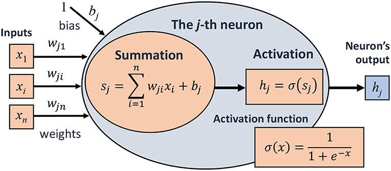
Figure 1. Schematic of an artificial neuron. Here, x_i and w_ji are inputs and corresponding weights, b_j is the neuron's bias (interpreted as a weight associated with a unit input), h_j is the neuron's output.

2.3. A Single-Hidden-Layer Feedforward Neural Network

Consider again Formula (1), where the right-hand side represents the result of an ANN with one hidden layer and one linear output unit. A combination of approximations of the form of Equation (1) will produce an ANN with several output units, which form the ANN's output layer (see Figure 2).

FIGURE 2

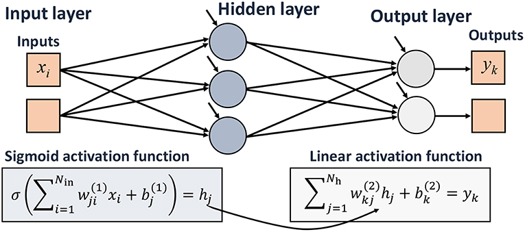
Figure 2. Schematic of a single-hidden-layer neural network.

Overall, a feedforward ANN consists of multiple neuron units (linked together by weighted connections) with activation functions each of which takes the neuron's net input, activates it, and produces a result that is used as input to another units. This type of ANN is called multilayer perceptron (MLP) (Priddy and Keller, 2005). Such ANNs are by far the most popular approximation technique. In the present review we make a special emphasis on feedforward multilayer neural networks, which are naturally suited for modeling. Reviews of other network types interesting for engineering applications are given by Meireles et al. (2003) and Zeng (1998).

Let N_in, N_h, and N_out denote the number of inputs, hidden neurons, and output units, respectively. Then, the number of learnable (or fitting) parameters is equal to N_h(N_in + N_out + 1) + N_out, provided the output layer uses biases. Observe (Sha and Edwards, 2007) that in practical applications like materials science or tribology, it is recommended to develop separate models for individual output properties, because training time dramatically increases with N_out. The number of inputs N_in is determined by the problem under consideration, that is by the available experimental data. It should be remembered (Bhadeshia, 1999) that neglect of an important input variable will lead to an increase in the noise associated with the ANN model's predictions. Finally, the number of hidden neurons N_h is a crucial factor that affects the ANN performance and is routinely a matter of trial and error, although there are some recommendations regarding how to choose N_h for given values of N_in and N_out (Gandomi and Roke, 2015).

2.4. Supervised Learning

Let an ANN be employed for modeling a tribological phenomenon, which is supposed to be characterized by a function y = f(x). It is clear that all particular information learned about the studied phenomenon will be stored in the values of the weights and biases that are the only fitting parameters. The process of evaluating appropriate weights and biases is called training (or learning by examples) and requires a training set of experimentally measured input-output examples (x^k, y^k), where x^k is an input vector, y^k is a corresponding output scalar, and k = 1, 2, …, N_train. The process of incorporating the available knowledge into the neural network is distinguished as supervised learning, because an external teacher (e.g., experimenter) provides the correct output y^k for each particular input x^k, that is y^k = f(x^k).

Let F(x) denote the ANN model prediction, so that F(x^k) is supposed to approximately predict the target value y^k, that is y^k ≈ F(x^k). Then, according to the least squares regression, the corresponding total training error can be computed as $\sum _{k=1}^{N_{\text{train}}}{\left(F({\text{x}}^k)-y^k\right)}^2$, and the training objective is to minimize the total error over the entire training set. As a result, one obtains an approximation F(x) for the sought-for function f(x). The practical implementation of this general algorithm requires numerical techniques for solving large-scale minimization problems.

Usually, MLPs are trained in an iterative way using the so-called back-propagation learning algorithm (Rumelhart et al., 1986), which utilizes the gradient descent method to update the values of weights and biases based on propagation of the output error F(x^k) − y^k through the network. Thus, as a result of each iteration, the network gradually learns from its error.

Finally, because usually an ANN is trained to be used for inputs that are different from the training examples, a separate testing set is required to assess the generalization capability of the ANN model (Bishop, 1995).

3. Applications of Neural Networks in Tribology

The use of ANNs in tribological applications was previously reviewed by Ripa and Frangu (2004), Rudnicki and Figiel (2002), and Velten et al. (2000). In this section, we make an emphasis on modeling aspect of ANN technique and overview recent advances in the field.

3.1. Modeling of Wear Rate and Friction Coefficient

It is widely accepted that an ANN model is likely to be a black-box model, since its interrelations between the inputs and outputs are difficult to interpret. Therefore, when applying ANN technique, an important question is that of choice of the input and output variables. To illustrate the major factors that should be accounted for in modeling of friction and wear, Figure 3 shows a schematic of the general construction of an ANN for tribological studies.

FIGURE 3

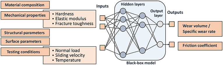
Figure 3. General schematic of ANN for correlating tribological properties with material parameters and testing conditions in sliding wear tests (after Friedrich et al., 2002).

It should be emphasized that the wear volume and the specific wear rate are extensive and intensive parameters, respectively. This, in particular, means that by choosing the wear volume as the ANN's output, it will be necessary to specify the sliding distance as one of the ANN's outputs. Further, experiments on fretting wear require the introduction of other relevant parameters such as number of cycles and tangential displacement amplitude (Kolodziejczyk et al., 2010).

It is of interest to observe that the specific wear rate (SWR) of graphene oxide (r-GO) reinforced Magnesium metal matrix composite was found to depend non-monotonically on the sliding distance (Kavimani and Prakash, 2017). At the same time, the effect of decrease in SWR is attributed to the reason that r-GO forms a self-lubricant layer on the composite surface, while the effect of further increase in SWR with the sliding distance is explained by loosening the bonding between the reinforcement and Mg matrix due to temperature increment within the composite surface. These interpretations of the ANN model can be supported by monitoring the coefficient of friction and the pin temperature in pin-on-disc wear testing.

We note that structural parameters such as the characteristic size of tested samples that determines the size of the contact zone may influence the test results as well, especially, for composite materials, which can reveal the multi-scale features in damage and wear (Jiang and Zhang, 2013). Note also that the wear track diameter was suggested to be employed (Banker et al., 2016) as one of the regression parameters to model the linear wear in pin-on-disc sliding tests, and it turned out to be more significant than load or pin-heating temperature. We observe that, whereas the interpretation of physical mechanisms underlying the input-output interrelations is challenging, special attention should be first directed to examining and explaining the input variable significance.

3.2. Hybrid Neural Network-Based Modeling

When utilizing an ANN for modeling purposes, many issues related to the implementation of the ANN, including the choice of its parameters (e.g., number of neurons in hidden layer) and a training algorithm, as well as a method of pre- and post-processing of input/output data, can be resolved in a more or less standard way (Priddy and Keller, 2005). A much more sensitive and perhaps most important issue is that of the ANN's type and architecture, especially in engineering applications, like tribological systems. In this respect, the selection of an appropriate ANN's architecture should be based on the developed understanding of related tribological phenomena.

Recently, Li et al. (2017) have shown that a hybrid neural network (HNN) model, which combines two types of ANNs, possesses remarkable capability for modeling tribological properties (see Figure 4). Specifically, along with a back-propagation (BP) network (this is another name for a MLP) it is suggested to make use of a radial basis function (RBF) network, while representing the model's target outputs as F_HNN(x) = μ₁F_BP(x) + μ₂F_RBF(x) with μ₁ and μ₂ being mixing coefficients. It is suggested to use a genetic algorithm (Gandomi and Roke, 2015) for training the HNN.

FIGURE 4

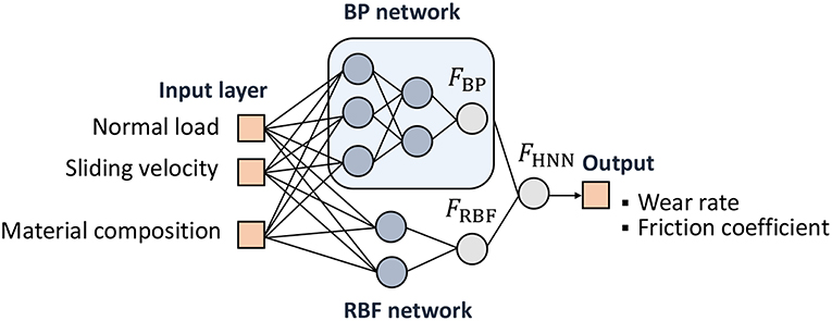
Figure 4. Structure of the hybrid neural network (Li et al., 2017).

Recall (Du and Swamy, 2006) that the output of the RBF network can be represented as follows (cf. Equation 1):

$\begin{array}{cc}F(x)={\displaystyle \sum _{j=1}^N{w}_j}\rho (\frac{\Vert x-c_j\Vert }{{\sigma }_j}).& (2)\end{array}$

Here, c_j is the center vector of the j-th kernel node, w_j and σ_j are its weight and smoothing factor, ∥x−c_j∥ is the Euclidean distance between the input x and the j-th node's center, and ρ(·) is the radial basis function, which is commonly taken to be Gaussian, that is ρ(x) = exp(−x²/2).

It is of practical interest to observe that since ρ(x) → 0 as x → ∞, the RBFs entering formula (2) are local to their center vectors c₁, c₂, …, c_N, so that a change of parameters of one certain kernel node, say c_k, will have a minor effect for all input values x whose distance ∥x−c_k∥ from the k-th node's center is relatively large. This means that RBF network has a strong capacity of local approximation.

It is also to note in this context, that in the case of modeling of microabrasion-corrosion process (Pai et al., 2008) an RBF based neural network has shown poor generalization capability compared to BP-MPL because it can memorize the input data. Radial basis function networks have been successfully employed for predicting the surface roughness in a turning process (Asiltürk and Çunkaş, 2011) and flank wear in drill (Panda et al., 2008).

3.3. Semi-physical NN Modeling for Fretting Wear

It is known (Estrada-Flores et al., 2006) that the black-box modeling approach, especially effective when the physical mechanisms underlying a studied phenomenon are either obscure or too complex for efficient first-principles modeling. The semi-physical (or the so-called “gray-box”) modeling approach combines the flexibility of the black-box approach with elements of available analytical modeling frameworks.

Recently, a semi-physical NN model was developed by Haviez et al. (2015) for fretting wear (see Figure 5). Their model introduces a two-level function approximation for the wear volume and utilizes the dissipated energy approach for getting insight into the mechanisms of fretting damage. The main advantage of this approach is that it reduces the number of fitting parameters compared to a standard ANN approach. This allows to cope with the issue of small data sets. On the other hand, incorporating prior knowledge of the fretting damage mechanisms into the NN modeling framework makes it easier to interpret the predicted results.

FIGURE 5

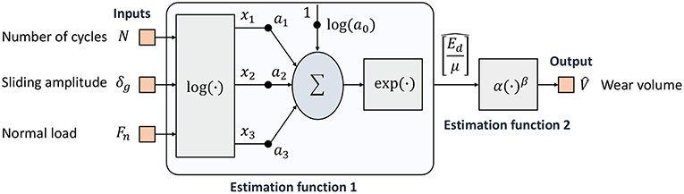
Figure 5. Schematic of the ANN-based semi-physical fretting wear model (Haviez et al., 2015).

4. Data-Driven Modeling Paradigm

In this section, we discuss important aspects that should be accounted for, when applying ANNs for modeling purposes. For this, we dwell on the relevant practical issues that arose in dealing with ANNs in tribology, materials science (Bhadeshia, 1999; Sha and Edwards, 2007), process engineering (Silva et al., 2006), hydrology (Dawson and Wilby, 2001), thermal science (Yang, 2008), and other mechanical engineering sectors (Zeng, 1998; Meireles et al., 2003).

4.1. Learning From Experiment

Generally speaking (Maier and Dandy, 2000), to build an artificial neural network, one needs three data sets, namely, training dataset (used to train the ANN), testing dataset (utilized to evaluate the predictive performance of the ANN model), and validation dataset (used to avoid the overfitting). The necessity in the latter appears when the number of learnable parameters (weights and biases) exceeds the number of training examples, so that the ANN can overfit the training data. In this case, the validation dataset is employed to control the ANN's fit on the training dataset during the learning (training) process and to stop training, when the ANN's error on the validation dataset starts to increase, thereby preventing overfitting of the training data (Maier and Dandy, 2000).

Usually, the validation and testing datasets are extracted from a set of experimental data in a random fashion. However, a care should be taken that at least the representativeness of each of the training and validation datasets has been achieved, and they have no overlaps with the training dataset. Observe that often the Taguchi approach is used to reduce the number of independent experiments by application of orthogonal arrays to the model factors, so that there will be an equal number of tests data points under each level of each of the ANN's input parameters (Teo and Sim, 1995). This means that besides an orthogonal training dataset, which is supposed to cover the ranges of inputs, one additionally needs independent data for cross-validating and testing the ANN model.

It should be emphasized that the quality of experimental data determines the soundness of the ANN model built upon the data. This, in particular, means that the accuracy of the ANN's predictions, generally, cannot be expected to be better than that of the row training data. At the same time, it is very important to give the errors for the testing dataset (Sha and Edwards, 2007).

4.2. Generalizing From Examples

Recall that, usually, each entry of the dataset is called an example. When an ANN, which is trained on a finite set of examples, is then applied to unseen inputs, its ability of accurate prediction is called generalization. From a function approximation point of view, such new examples can be regarded as either interpolation or extrapolation of the training data. With respect to neural networks, the operation of interpolation is preferred over extrapolation (Flood and Kartam, 1994). Therefore, it is recommended that the training examples should span the domain of interest completely (Liu et al., 1993). In other words, by and large, ANNs should not be applied for generalization outside the convex hull of the training dataset. In particular, when preparing the training dataset, it is recommended (Yin et al., 2003) to include examples with maximum or minimum values of any input, while the remaining experimental examples are then grouped randomly into the training dataset, the testing dataset, and if needed, the validation dataset. Sha and Edwards (2007) discussed the problems regularly encountered in applying neural networks and a growing tendency for the misapplication of ANN methodology. They have recommended suitable guidelines for the proper handling of ANNs to reveal their potential for effective modeling and analysis when using limited data for training and testing.

4.3. Inherent Nonlinearity

Modeling of nonlinear relationships using the ANN methodology is generally seen to be simpler in comparison to a nonlinear regression approach (Zeng, 1998; Paliwal and Kumar, 2009). Considering the tool wear in hard machining process, Quiza et al. (2013) compared the analysis of the data based on MLP type neural networks and statistical (linear, quadratic, and potential) models to conclude that the neural network model has shown better capability for accurate predictions.

Observe that nonlinear behavior of the neural network is introduced by the sigmoidal activation function of the hidden neurons. For any inputs to a hidden neuron, the activation function maps their linear combination into a specific interval [e.g., (0, 1) in the case of the sigmoid function and (−1, 1) in the case of the hyperbolic tangent activation function σ(x) = (e^x − e^−x)/(e^x + e^−x)]. It should be remembered that, if a nonlinear activation function is employed in the output layer, then the output data should be normalized according to the range interval of this activation function.

The inherent nonlinearity of ANNs has been exploited to develop powerful models for various physical phenomena (Maren et al., 2014). On the other hand, it should be noted that the inherent nonlinearity of neural networks implies the existence of many sub-optimal networks, which correspond to the local minima of the error function. Therefore, it should be expected that depending on the initial randomization of neural network weights and biases, common training algorithms can converge to different sub-optimal networks (Beliakov and Abraham, 2002), especially when the stopping criterion relies on a validation dataset.

4.4. ANN Modeling Approach

As pointed out by Yang (2008), ANNs have a strong capacity for accurate recognizing the inherent relationship between any sets of inputs and outputs without formulating a physical model of a phenomenon under consideration. Moreover, given a large amount of experimental data, the ANN model does account for all the physical mechanisms relating the outputs to the inputs. At the same time, a priori physical insight to the phenomenon is necessary to determine the proper input parameters.

Recall that modeling is a mathematical framework used to describe the physical principles underlying the interrelations between the input and the output of a system. With respect to industrial applications, the non-algorithmic ability of ANNs to approximate the input to output mapping independent of the size and complexity of the system is of great use (Meireles et al., 2003).

Observe (Dawson and Wilby, 2001) that ANNs can be classified as parametric models that are generally lumped (or homogeneous), because they incorporate no information about the spatial distribution of inputs and outputs, and predict only the spatially averaged response. Indeed, the contact pressure at a sliding interface may vary spatially over the area of contact as well as the linear wear rate, especially in fretting. However, the known ANN models of fretting wear operate with the total contact load and the wear rate, which are integrals of the former distributed characteristics over the contact area.

It is to note that the ANN model design does not end with the model's implementation, and a number of algorithms (Gevrey et al., 2003) can be afterwards used to analyze the relative contribution (significunce) of the model variables. The generalization capability of ANN solutions can be improved by extracting rules using the connection strength in the network (Andrews et al., 1995), thereby identifying regions in input space, which are not represented sufficiently in the training dataset used for the knowledge initialization, i.e., which are overlooked when inserting knowledge into the ANN.

Since a trained ANN is represented by a composition of analytical functions, the ANN model can be readily used to investigate the effect of each input individually, whereas this may be very difficult to do experimentally (Bhadeshia, 1999). It is also to note (Craven and Shavlik, 1994) that ANNs may discover salient features in the input data whose importance was not previously recognized. It has, for instance, very recently been shown by Verpoort et al. (2018) that elongation, as a measure of the materials ability to deform plastically, is the material property most strongly correlated to fracture toughness, which, in turn, is known to play a certain role in the wear of metals (Hornbogen, 1975).

4.5. Adaptability and Robustness

It is recognized that the performance of an ANN model strongly depends on the network architecture (Gandomi and Roke, 2015), and it can be assessed using a number of unit-free performance measures. On the other hand, the performance efficiency of a neural network depends on the quality of information gained in the training process performed on a finite number of examples. Therefore, when an additional dataset becomes available for processing, the network's weights and biases can be updated to accumulate the newly provided experimental evidence. This feature of ANNs is especially useful for the design of on-line monitoring systems. As an example of the ANN adaptability, Ghasempoor et al. (1998) and Silva et al. (2006) developed ANN-based intelligent condition monitoring systems for on-line estimation of tool wear from the changes occurring in the cutting force signals by implementing a continuous on-line training to guarantee the adjustability of the ANN model to variations in cutting conditions, when they fall outside of the neural network's trained zone.

Finally, let us underline once again that the effectiveness/robustness of the ANN model crucially depends on the amount and generality of the training data. As it was observed by Pai et al. (2008), when employing neural networks for modeling of micro-abrasion and tribo-corrosion, it should be taken into account that there is extensive expected influence of the interplay between the model parameters in their various levels. Yet another condition for efficient implementation and application of a data-driven model is the absence of significant changes to the system under consideration during the period covered by the model (Solomatine et al., 2008).

5. Conclusion

ANNs is a promising mathematical technique that can be used for modeling (in a general sense of this term) complex tribological phenomena. Without doubts, an ANN modeling methodology will be increasingly integrated into tribological studies, provided prior knowledge about tribological systems and insights into the physics of tribological processes has been incorporated into the ANN model.

Author Contributions

The author confirms being the sole contributor of this work and has approved it for publication.

Conflict of Interest Statement

The author declares that the research was conducted in the absence of any commercial or financial relationships that could be construed as a potential conflict of interest.

Footnotes

1. ^The English translation of the original paper by V.A. Zhuravlev was published as a historical paper (Zhuravlev, 2007) in the Journal of Engineering Tribology.

References

Aleksendrić, D., and Barton, D. (2009). Neural network prediction of disc brake performance. Tribol. Int. 42, 1074–1080. doi: 10.1016/j.triboint.2009.03.005

CrossRef Full Text | Google Scholar

Ali, Y., Rahman, R., and Hamzah, R. (2014). Acoustic emission signal analysis and artificial intelligence techniques in machine condition monitoring and fault diagnosis: a review. J. Teknol. 69, 121–126. doi: 10.11113/jt.v69.3121

CrossRef Full Text | Google Scholar

Andrews, R., Diederich, J., and Tickle, A. (1995). Survey and critique of techniques for extracting rules from trained artificial neural networks. Knowl. Based Syst. 8, 373–389. doi: 10.1016/0950-7051(96)81920-4

CrossRef Full Text | Google Scholar

Argatov, I., and Fadin, Y. (2010). Asymptotic modeling of the long-period oscillations of tribological parameters in the wear process of metals under heavy duty sliding conditions with application to structural health monitoring. Int. J. Eng. Sci. 48, 835–847. doi: 10.1016/j.ijengsci.2010.05.006

CrossRef Full Text | Google Scholar

Asiltürk, İ., and Çunkaş, M. (2011). Modeling and prediction of surface roughness in turning operations using artificial neural network and multiple regression method. Exp. Syst. Appl. 38, 5826–5832. doi: 10.1016/j.eswa.2010.11.041

CrossRef Full Text | Google Scholar

Banker, V., Mistry, J., Thakor, M., and Upadhyay, B. (2016). Wear behavior in dry sliding of inconel 600 alloy using taguchi method and regression analysis. Procedia Technol. 23, 383–390. doi: 10.1016/j.protcy.2016.03.041

CrossRef Full Text | Google Scholar

Bao, J., Tong, M., Zhu, Z., and Yin, Y. (2012). “Intelligent tribological forecasting model and system for disc brake,” in 2012 24th Chinese Control and Decision Conference (CCDC), 3870–3874. doi: 10.1109/CCDC.2012.6243100

CrossRef Full Text | Google Scholar

Barber, J. (2018). Contact Mechanics. New York, NY: Springer.

PubMed Abstract | Google Scholar

Beliakov, G., and Abraham, A. (2002). “Global optimisation of neural networks using a deterministic hybrid approach,” in Hybrid Information Systems. Advances in Soft Computing, Vol. 14, eds A. Abraham and M. Köppen (Heidelberg: Physica), 79–92.

Google Scholar

Bhadeshia, H. (1999). Neural networks in materials science. ISIJ int. 39, 966–979. doi: 10.2355/isijinternational.39.966

CrossRef Full Text | Google Scholar

Bhushan, B., Israelachvili, J., and Landman, U. (1995). Nanotribology: friction, wear and lubrication at the atomic scale. Nature 374, 607–616. doi: 10.1038/374607a0

CrossRef Full Text | Google Scholar

Bishop, C. (1995). Neural Networks for Pattern Recognition. Oxford: Oxford University Press.

Google Scholar

Borodich, F. (2013). “Fractal contact mechanics,” in Encyclopedia of Tribology, eds Q. Wang and Y.-W. Chung (Boston, MA: Springer), 1249–1258. doi: 10.1007/978-0-387-92897-5_512

CrossRef Full Text | Google Scholar

Borodich, F., Keer, L., and Harris, S. (2002). Self-similarity in abrasiveness of hard carbon-containing coatings. J. Tribol. 125, 1–7. doi: 10.1115/1.1509773

CrossRef Full Text | Google Scholar

Bowden, F., and Tabor, D. (1986). The Friction and Lubrication of Solids. Oxford: Clarendon Press.

Google Scholar

Bucholz, E., Kong, C., Marchman, K., Sawyer, W., Phillpot, S., Sinnott, S., et al. (2012). Data-driven model for estimation of friction coefficient via informatics methods. Tribol. Lett. 47, 211–221. doi: 10.1007/s11249-012-9975-y

CrossRef Full Text | Google Scholar

Craven, M., and Shavlik, J. (1994). “Using sampling and queries to extract rules from trained neural networks,” in Machine Learning Proceedings 1994, eds W. Cohen and H. Hirsh (San Francisco, CA: Morgan Kaufmann), 37–45.

Google Scholar

Cybenko, G. (1989). Approximation by superpositions of a sigmoidal function. Math. Control Sign. Syst. 2, 303–314. doi: 10.1007/BF02551274

CrossRef Full Text | Google Scholar

Dawson, C., and Wilby, R. (2001). Hydrological modelling using artificial neural networks. Progr. Phys. Geogr. Earth Environ. 25, 80–108. doi: 10.1177/030913330102500104

CrossRef Full Text | Google Scholar

Dowla, F., and Rogers, L. (1995). Solving Problems in Environmental Engineering and Geosciences with Artificial Neural Networks. Cambridge, MA: MIT Press.

Google Scholar

Du, K.-L., and Swamy, M. (2006). “Radial basis function networks,” in Neural Networks in a Softcomputing Framework (Springer, London), 251–294.

Google Scholar

Estrada-Flores, S., Merts, I., De Ketelaere, B., and Lammertyn, J. (2006). Development and validation of “grey-box” models for refrigeration applications: a review of key concepts. Int. J. Refrigerat. 29, 931–946. doi: 10.1016/j.ijrefrig.2006.03.018

CrossRef Full Text | Google Scholar

Flood, I., and Kartam, N. (1994). Neural networks in civil engineering. i: Principles and understanding. J. Comput. Civil Eng. 8, 131–148. doi: 10.1061/(ASCE)0887-3801(1994)8:2(131)

CrossRef Full Text | Google Scholar

Friedrich, K., Reinicke, R., and Zhang, Z. (2002). Wear of polymer composites. Proc. Inst. Mech. Eng. J. 216, 415–426. doi: 10.1243/135065002762355334

CrossRef Full Text | Google Scholar

Gandomi, A., and Roke, D. (2015). Assessment of artificial neural network and genetic programming as predictive tools. Adv. Eng. Softw. 88, 63–72. doi: 10.1016/j.advengsoft.2015.05.007

CrossRef Full Text | Google Scholar

Gevrey, M., Dimopoulos, I., and Lek, S. (2003). Review and comparison of methods to study the contribution of variables in artificial neural network models. Ecol. Model. 160, 249–264. doi: 10.1016/S0304-3800(02)00257-0

CrossRef Full Text | Google Scholar

Ghasempoor, A., Moore, T., and Jeswiet, J. (1998). On-line wear estimation using neural networks. Proc. Inst. Mech. Eng. B 212, 105–112. doi: 10.1243/0954405971515537

CrossRef Full Text | Google Scholar

Goryacheva, I. (1998). Contact Mechanics in Tribology. Dordrecht: Kluwer Acad. Publ.

Greenwood, J., and Williamson, J. (1966). Contact of nominally flat surfaces. Proc. R. Soc. Lond. A 295, 300–319. doi: 10.1098/rspa.1966.0242

CrossRef Full Text | Google Scholar

Haviez, L., Toscano, R., El Youssef, M., Fouvry, S., Yantio, G., and Moreau, G. (2015). Semi-physical neural network model for fretting wear estimation. J. Intel. Fuzzy Syst. 28, 1745–1753. doi: 10.3233/IFS-141461

CrossRef Full Text | Google Scholar

Haykin, S. (1999). Neural Networks: A Comprehensive Foundation. Upper Saddle River, NJ: Prentice-Hall.

Google Scholar

Hills, D., and Nowell, D. (1994). Mechanics of Fretting Fatigue. Dordrecht: Kluwer.

Google Scholar

Hornbogen, E. (1975). The role of fracture toughness in the wear of metals. Wear 33, 251–259. doi: 10.1016/0043-1648(75)90280-X

CrossRef Full Text | Google Scholar

Hornik, K., Stinchcombe, M., and White, H. (1989). Multilayer feedforward networks are universal approximators. Neural Netw. 2, 359–366. doi: 10.1016/0893-6080(89)90020-8

CrossRef Full Text | Google Scholar

Jiang, Z. and Zhang, Z. (2013). “Wear of multi-scale phase reinforced composites,” in Tribology of Nanocomposites. Materials Forming, Machining and Tribology, ed J. Davim (Berlin; Heidelberg: Springer), 79–100.

PubMed Abstract | Google Scholar

Jiang, Z., Zhang, Z., and Friedrich, K. (2007). Prediction on wear properties of polymer composites with artificial neural networks. Composites Sci. Technol. 67, 168–176. doi: 10.1016/j.compscitech.2006.07.026

CrossRef Full Text | Google Scholar

Johnson, K. (1985). Contact Mechanics. Cambridge: Cambridge University Press.

Google Scholar

Jones, S., Jansen, R., and Fusaro, R. (1997). Preliminary investigation of neural network techniques to predict tribological properties. Tribol. Trans. 40, 312–320. doi: 10.1080/10402009708983660

CrossRef Full Text | Google Scholar

Kadi, H. (2006). Modeling the mechanical behavior of fiber-reinforced polymeric composite materials using artificial neural networks—a review. Composite Struct. 73, 1–23. doi: 10.1016/j.compstruct.2005.01.020

CrossRef Full Text | Google Scholar

Kavimani, V., and Prakash, K. (2017). Tribological behaviour predictions of r-go reinforced mg composite using ann coupled taguchi approach. J. Phys. Chem. Solids 110, 409–419. doi: 10.1016/j.jpcs.2017.06.028

CrossRef Full Text | Google Scholar

Kolodziejczyk, T., Toscano, R., Fouvry, S., and Morales-Espejel, G. (2010). Artificial intelligence as efficient technique for ball bearing fretting wear damage prediction. Wear 268, 309–315. doi: 10.1016/j.wear.2009.08.016

CrossRef Full Text | Google Scholar

Kragelsky, I., Dobychin, M., and Kombalov, V. (1982). Friction and Wear. Calculation Methods. Oxford: Pergamon Press.

Google Scholar

Li, D., Lv, R., Si, G., and You, Y. (2017). Hybrid neural network-based prediction model for tribological properties of polyamide6-based friction materials. Polym. Composites 38, 1705–1711. doi: 10.1002/pc.23740

CrossRef Full Text | Google Scholar

Li, J., Zhang, J., Ge, W., and Liu, X. (2004). Multi-scale methodology for complex systems. Chem. Eng. Sci. 59, 1687–1700. doi: 10.1016/j.ces.2004.01.025

CrossRef Full Text | Google Scholar

Liao, S.-H., Chu, P.-H., and Hsiao, P.-Y. (2012). Data mining techniques and applications–a decade review from 2000 to 2011. Exp. Syst. Appl. 39, 11303–11311. doi: 10.1016/j.eswa.2012.02.063

CrossRef Full Text | Google Scholar

Liu, Y., Upadhyaya, B., and Naghedolfeizi, M. (1993). Chemometric data analysis using artificial neural networks. Appl. Spectrosc. 47, 12–23. doi: 10.1366/0003702934048406

CrossRef Full Text | Google Scholar

Maier, H., and Dandy, G. (2000). Neural networks for the prediction and forecasting of water resources variables: a review of modelling issues and applications. Environ. Model. Softw. 15, 101–124. doi: 10.1016/S1364-8152(99)00007-9

CrossRef Full Text | Google Scholar

Maren, A., Harston, C., and Pap, R. (2014). Handbook of Neural Computing Applications. San Diego, CA: Academic Press.

Google Scholar

Meireles, M., Almeida, P., and Simoes, M. (2003). A comprehensive review for industrial applicability of artificial neural networks. IEEE Tran. Ind. Electron. 50, 585–601. doi: 10.1109/TIE.2003.812470

CrossRef Full Text | Google Scholar

Nayak, P. (1971). Random process model of rough surfaces. J. Lubric. Technol. 93, 398–407. doi: 10.1115/1.3451608

CrossRef Full Text | Google Scholar

Pai, P., Mathew, M., Stack, M., and Rocha, L. (2008). Some thoughts on neural network modelling of microabrasion–corrosion processes. Tribol. Int. 41, 672–681. doi: 10.1016/j.triboint.2007.11.015

CrossRef Full Text | Google Scholar

Paliwal, M., and Kumar, U. (2009). Neural networks and statistical techniques: a review of applications. Exp. Syst. Appl. 36, 2–17. doi: 10.1016/j.eswa.2007.10.005

CrossRef Full Text | Google Scholar

Panda, S., Chakraborty, D., and Pal, S. (2008). Flank wear prediction in drilling using back propagation neural network and radial basis function network. Appl. Soft Comput. 8, 858–871. doi: 10.1016/j.asoc.2007.07.003

CrossRef Full Text | Google Scholar

Popov, V. (2017). Contact Mechanics and Friction. Berlin: Springer-Verlag.

PubMed Abstract | Google Scholar

Popov, V., and Heß, M. (2015). Method of Dimensionality Reduction in Contact Mechanics and Friction. Berlin; Heidelberg: Springer-Verlag.

Google Scholar

Popov, V., and Psakhie, S. (2007). Numerical simulation methods in tribology. Tribol. Int. 40, 916–923. doi: 10.1016/j.triboint.2006.02.020

CrossRef Full Text | Google Scholar

Priddy, K., and Keller, P. (2005). Artificial Neural Networks: An Introduction. Bellingham, WA: SPIE Press.

Google Scholar

Quiza, R., Figueira, L., and Davim, J. (2013). Comparing statistical models and artificial neural networks on predicting the tool wear in hard machining d2 aisi steel. Int. J. Adv. Manuf. Technol. 37, 641–648. doi: 10.1007/s00170-007-0999-7

CrossRef Full Text | Google Scholar

Ripa, M., and Frangu, L. (2004). A survey of artificial neural networks applications in wear and manufacturing processes. J. Tribol. 35–42.

Google Scholar

Rudnicki, Z., and Figiel, W. (2002). Neural nets applications in tribology research. Zagadnienia Eksploatacji Maszyn 37, 97–110. Available online at: https://www.infona.pl/resource/bwmeta1.element.baztech-article-BOS3-0008-0077

Google Scholar

Rumelhart, D., Hinton, G., and Williams, R. (1986). Learning representations by back-propagating errors. Nature 323, 533–536. doi: 10.1038/323533a0

CrossRef Full Text | Google Scholar

Sha, W., and Edwards, K. (2007). The use of artificial neural networks in materials science based research. Mater. Design 28, 1747–1752. doi: 10.1016/j.matdes.2007.02.009

CrossRef Full Text | Google Scholar

Shebani, A., and Iwnicki, S. (2018). Prediction of wheel and rail wear under different contact conditions using artificial neural networks. Wear 406-407:173–184. doi: 10.1016/j.wear.2018.01.007

CrossRef Full Text | Google Scholar

Silva, R., Wilcox, S., and Reuben, R. (2006). Development of a system for monitoring tool wear using artificial intelligence techniques. Proc. Inst. Mechan. Eng. B 220, 1333–1346. doi: 10.1243/09544054JEM328

CrossRef Full Text | Google Scholar

Solomatine, D., See, L., and Abrahart, R. (2008). “Data-driven modelling: concepts, approaches and experiences,” in Practical Hydroinformatics: Computational Intelligence and Technological Developments in Water Applications, eds R. Abrahart, L. See and D. Solomatine (Berlin; Heidelberg: Springer Berlin Heidelberg), 17–30.

Google Scholar

Teo, M.-Y., and Sim, S.-K. (1995). Training the neocognitron network using design of experiments. Artif. Intel. Eng. 9, 85–94. doi: 10.1016/0954-1810(95)95752-R

CrossRef Full Text | Google Scholar

Vakis, A., Yastrebov, V., Scheibert, J., Nicola, L., Dini, D., Minfray, C., et al. (2018). Modeling and simulation in tribology across scales: an overview. Tribol. Int. 125, 169–199. doi: 10.1016/j.triboint.2018.02.005

CrossRef Full Text | Google Scholar

Velten, K., Reinicke, R., and Friedrich, K. (2000). Wear volume prediction with artificial neural networks. Tribol. Int. 33, 731–736. doi: 10.1016/S0301-679X(00)00115-8

CrossRef Full Text | Google Scholar

Verpoort, P., MacDonald, P., and Conduit, G. (2018). Materials data validation and imputation with an artificial neural network. Comput. Mater. Sci. 147, 176–185. doi: 10.1016/j.commatsci.2018.02.002

CrossRef Full Text | Google Scholar

Waszczyszyn, Z. (1999). “Fundamentals of artificial neural networks,” in Neural Networks in the Analysis and Design of Structures, ed Z. Waszczyszyn (Wien: Springer-Verlag), 1–51.

Google Scholar

Whitehouse, D. (2001). Fractal or fiction. Wear 249, 345–353. doi: 10.1016/S0043-1648(01)00535-X

CrossRef Full Text | Google Scholar

Xu, Y., and Jackson, R. (2018). Boundary element method (bem) applied to the rough surface contact vs. bem in computational mechanics. Friction 6, 1–13. doi: 10.1007/s40544-018-0229-3

CrossRef Full Text | Google Scholar

Yang, K. (2008). Artificial neural networks (anns): a new paradigm for thermal science and engineering. ASME J. Heat Transfer 130, 093001–093001–19. doi: 10.1115/1.2944238

CrossRef Full Text | Google Scholar

Yevtushenko, A. A., and Grzes, P. (2010). The fem-modeling of the frictional heating phenomenon in the pad/disc tribosystem (a review). Numeric. Heat Transfer A 58, 207–226. doi: 10.1080/10407782.2010.497312

CrossRef Full Text | Google Scholar

Yin, C., Rosendahl, L., and Luo, Z. (2003). Methods to improve prediction performance of ann models. Simulat. Model. Pract. Theory 11, 211–222. doi: 10.1016/S1569-190X(03)00044-3

CrossRef Full Text | Google Scholar

Zeng, P. (1998). Neural computing in mechanics. Appl. Mech. Rev. 51, 173–197. doi: 10.1115/1.3098995

CrossRef Full Text | Google Scholar

Zhang, Z., Barkoula, N.-M., Karger-Kocsis, J., and Friedrich, K. (2003). Artificial neural network predictions on erosive wear of polymers. Wear 255, 708–713. doi: 10.1016/S0043-1648(03)00149-2

CrossRef Full Text | Google Scholar

Zhuravlev, V. (1940). On the question of theoretical justification of the amontons–coulomb law for friction of unlubricated surfaces. J. Techn. Phys. 10, 1447–1452.

Google Scholar

Zhuravlev, V. (2007). On the question of theoretical justification of the amontons–coulomb law for friction of unlubricated surfaces. Proc. Inst. Mech. Eng. J. 221, 893–898. doi: 10.1243/13506501JET176

CrossRef Full Text | Google Scholar