Abstract
A new concept of the effective surface profile is proposed to facilitate the prediction of the worn surface texture at sliding friction. The effective surface profile is a 2D height characteristic that consists of the asperities of surface superimposed on a plane perpendicular both to the mean surface plane and to the direction of sliding. We hope to present a clear and compelling argument favoring the use of the effective surface profile as a versatile tool for characterization of rough surfaces at abrasive wear, calculation of contact characteristic at sliding friction, and for prediction of evolution of roughness parameters from virgin to the worn surfaces. The effective surface profile can be successfully applied for investigations of sliding abrasive wear under dry or lubricated conditions.
Introduction
Prediction of wear of materials at sliding is an important but complex challenge (Zmitrowicz, 2006; Manier et al., 2008; Lu et al., 2014). General analytical models (Kato, 2002) predicting a wear mode under various conditions are complicated (Hsu et al., 1997). Wear is defined as damage to one or both surfaces involved in friction. In most of cases, wear is characterized by the presence of tracks that have a measurable width, depth, as well as different surface roughness and texture inside of worn area. The wear profile describes the irreversible changes of a worn surface, and it is a useful measure of surface damage. Based on many experimental evidences of wear examinations (Archard, 1953; Bowden and Tabor, 1964; Glaeser, 1992), the main mechanisms of wear have been identified as asperity interlocking, plowing, and cutting of surface (Bowden and Tabor, 1964).
The objective of wear modeling depends on its application. In most of cases, the main aim of the wear modeling is to predict the volume loss depending on mechanical properties of contacting solids and the tribotesting schemes used. Perhaps, the first attempt to summarize the proposed wear models was done by Meng and Ludema (1995). They have performed classification of wear models and have distinguished three main types of wear equations: empirical, phenomenological and those based on the selected failure mechanism. The main equation allowing to calculate the loss of material is the Archard wear equation (Archard, 1953) or so called Archard's law which is a simple calculation procedure of wear volume and widely used in engineering calculations.
Another challenge is to predict the evaluation of worn surface structure and its roughness parameters occurred at abrasive wear, grinding, milling and turning processes. Study of the ground surface roughness is an important issue for tribological applications because it impacts the performance of machine elements. The virtual reality technology was used by Gong et al. (Gong et al., 2002) to simulate the grinding process. They found that the average roughness Ra on the ground workpiece can be estimated by the arithmetic average of contour absolute values in a sampling length of workpiece. Aslan and Budak (2015) have proposed grinding model with thermo-mechanical material deformation allowing to simulate abrasive wheel topography and to obtain the final workpiece surface profile. The abrasion simulation considers three types of interactions such as rubbing, plowing, and cutting. The main point of abrasion simulation is that not all the grits are involved into the process, but some of them exceeding the certain cut-off height and these acting grits are distributed randomly within the working area. Simulating the abrasive wear by parallel scratches, da Silva and de Mello (2009) have used the load map that represents combination of position and normal load of scratches being generated and this load map closely correlates to the average profile of the reference surface used in simulation. It allows predicting the roughness parameters with good accuracy. Similar approach was proposed by Shahabi and Ratnam (2016) for determining the final surface profile of workpieces in finish turning. They have shown that final surface profile formed by the flank wear of cutting tool and the surface roughness could be predicted knowing the shape of the tool cutting edge.
In most of investigations of the contact of rough surfaces, roughness parameters are considered as characterizing the mating surfaces (Borodich and Bianchi, 0000; Borodich et al., 2016). Mainly, the analytical models consider the specific type of wear, as it was proposed by Goryacheva for fatigue wear (Goryacheva, 1998) or Popov and Pohrt for adhesive wear (Popov and Pohrt, 2018). Also, there is no simple analytical method or technique that involves the initial surface topography to allow predicting the evolution of worn surface structure or texture that occurs during the abrasive or plowing wear process.
The commonly used roughness parameters in tribology are the arithmetic average height (Ra), root mean square (Rq), skewness (Rsk), and kurtosis (Rku). The correlation between the surface roughness and friction behavior has been recognized for a long time, however until now it is still an unsolved challenge. The variation of surface parameters during the running-in wear stage, where the mutual transition between different types of wear exists, was deeply investigated by Jeng (Jeng and Gao, 2000; Jeng et al., 2004) especially for engine bore surfaces. He has found that Rq became lower and Rsk got negative after sliding wear, and these results are correct for different original surface height distributions. The surface roughness evolution in sliding process has been studied by Yuan et al. (2008). The results have shown that Ra and Rq values of test samples first decreased from the running-in to steady wear stage and then increased from the steady wear to severe wear stage. However, variation of roughness parameters when initial surface undergoes the transformation during wear is still not investigated in details.
A lot of previous theoretical and experimental studies of friction and wear have formed the main basis of surface transformation during a sliding friction of rough surfaces. During sliding, the deformation of surface can be entirely elastic. In such a case the wear is absent. With an increase of external load, the deformation mode changes to plastic one and the surface layer of material displaced by the passage of an asperity is being plowed into side ridges. Such representation was used in several models of wear (Kapoor and Johnson, 1992, 1994), where the plowing is the dominating factor (Challen et al., 1984; Xie and Williams, 1996). The steady state sliding of rough surfaces that considers the groove formation in presence of elastic and plastic “shakedown limit” was also analyzed (Kapoor et al., 1994). However, the height change of initial rough surface was taken into account based on the roughness of a surface profile only. Thus, the analysis of evolution of worn surface topography, where the initial surface structure is considered, have not been reported yet.
In this paper, a concept of effective surface profile (ESP), which is the superimposed asperities of initial hard rough surface along the direction of sliding, is presented with the aim of predicting the worn surface structure, corresponding roughness parameters, and contact characteristics under abrasive sliding conditions.
Conventional Contact Characterization
Surface Roughness Parameters
Set of roughness parameters for a single line (profile) characterization can be divided to three main groups (Dong et al., 1992, 1993, 1994a,b; Stout, 1993; Jiang et al., 2007a,b) according to its functional properties: (1) amplitude parameters, (2) spacing parameters, and (3) hybrid parameters. According to the classification presented elsewhere (Gadelmawla et al., 2002), for roughness characterization from a profile data, total of 41 parameters, including 20 amplitude parameters, 8 spacing parameters, and 13 hybrid parameters, can be utilized. To point out which of these various parameters is the most relevant one to describe the surface transformation due to friction and wear is ambiguous and can be a pointless task.
Let us describe the main amplitude (height) parameters that commonly used for a roughness characterization. Taking into account the absence of difference of statistical meaning for equations applying for calculation of the roughness, only the capital letter “S” will be used for profile and surface parameters.
Arithmetic Average Height
The arithmetic average height parameter Ra or Sa is defined as the average deviation of the roughness irregularities from the mean line over the sampling length l, or from a mean surface over the nominal surface in case of areal characterization. The main weakness is that Ra or Sa give no information on the profile shape or texture of surface and they are not sensitive to the fine changes of asperity peaks and depths of valleys. These roughness parameters describe the average value of height deviation along the Z axis regardless how a height data was collected, along a linear profile or surface.
Root Mean Square
This parameter is the standard deviation of the distribution of profile or surface height points relating to the mean line. Rq (Sq) parameter is more sensitive to the changes of height amplitudes.
Skewness
The skewness qualifies the symmetry of height distribution about the mean line for a profile or mean plane for a surface. For the Gaussian distribution, which has a symmetrical “bell-like” shape, the Ssk is zero. For asymmetric distribution of profile/surface heights, the Ssk may be negative or positive. Ssk is positive if a surface has many peaks and small number of valleys. The negative Ssk indicates that the quantity or deepness of valleys dominate over peaks above the mean plane.
Kurtosis
The kurtosis qualifies the flatness of the height distribution curve. The profile or surface with a Gaussian distribution of height points has a kurtosis of 3. Centrally distributed surfaces has a kurtosis value larger than 3, whereas the kurtosis of a well spread distribution is smaller than 3.
Ssk and Sku are more sensitive to the fine changes of topography than Ra and Rq, and they are used in the comparable analysis of worn surface topography (Jeng and Gao, 2000; Yuan et al., 2008).
The height roughness parameters listed above are widely used in surface characterization of worn surfaces, however, as it will be shown in this manuscript, cannot describe the evolution of surface parameters during wear.
Contact of Rough Surfaces
The basis of statistical description and corresponding classical model of contacting rough surfaces has been proposed in 1966 by Greenwood and Williamson (1966). They have shown the Gaussian distribution of heights on many surface profiles. Moreover, it was found that the distribution of asperity peaks is close to Gaussian distribution too, and both the mean value and the standard deviation of asperity peaks differ from that of heights. It should be noted here that Zhuravlev has published in 1940 the pioneering work related to the contact mechanics, where the statistical approach for describing the surface roughness was proposed. He considered a linear distribution of heights of aligned spherical asperities and yielded an almost linear relation between external load P and real contact area Ar. The translation of a historical Zhuravlev's paper has been done by Borodich (Zhuravlev, 2007) and discussed elsewhere (Borodich et al., 2016; Borodich and Savencu, 2017).
The mentioned above GW model is widely used for calculation of the bearing capacity of contacting surfaces (Bhushan, 1998, 2001). However, as it will be shown in section Contact of Rough Surfaces, GW theory describes the static contact of rough surfaces and could not correspond to the contact geometry occurred due to the repeatable sliding movements of surfaces. Here, we briefly list the main equations of GW theory and these equations will be discussed with equations derived with the help of effective surface profile in section Contact of Rough Surfaces.
The GW model was defined by three parameters: σ is the standard deviation of the asperity peak distribution; R is the radius of curvature of the asperities; n is the density of asperities per unit area. According to the GW model, the distribution density function of peak heights is of the form:
where z is the peak height. If two surfaces are brought into contact until their nominal planes are separated by a distance d, then there will be a contact at any asperity whose height is greater than distance d. Thus, if a rough surface has N asperities, the expected number of contacting asperities is:
Therefore, if the surfaces come to contact with a compression of δ = z − d, and all asperities undergo the elastic deformation according to the prediction of Hertzian theory, then, per unit nominal area, the real area of contact and the applied load will be:
where E* is the composite elastic modulus of contacting rough bodies.
GW model is widely used in contact problems for predicting the normal contact of surface (Adams and Nosonovsky, 2000) and it has many variations for certain problems (Greenwood and Wu, 2001; Borodich et al., 2016). Also, GW model is often considered when the sliding friction of rough surfaces is modeled (Kapoor et al., 1994; Xie and Williams, 1996). However, the GW model is applicable for pure elastic contact only. In case of elastoplastic or pure plastic interaction typical for abrasive or plowing wear at sliding the application of GW model has to be revised.
Numerical Investigations Details
Running-in state exists at the beginning of a wear test in which the contacting surfaces experience an initial wear, resulting in the adaptation of surfaces accompanying by volume loss, after which the slope of wear curve declines reaching the steady state.
In our numerical investigation we consider an ideal case of sliding friction of rough hard surface against softer one. In fact, this corresponds to the sliding friction of hard coatings such as DLC against softer materials as metals or ceramics (Hayward et al., 1992) where the friction coefficient tends to be high, since asperities of the coating surface work as abrasives.
In numeric experiments nominally rough surface initially was shifted down according the selected vertical displacement Δz and was continuously moved over the soft surface subjected to wear. Several wear mechanisms could be involved in the groove formation on the surface of softer material. The transformation of wear surface represents how the surface of soft material would be expected to change during the repeated sliding mainly accompanied by the plowing and cutting. However, wear mechanisms were thoroughly maintained in our computer simulation, because the main aim of our idealization is to investigate the final surface topography at given conditions of sliding, rather than the specific wear mechanism and mechanical behavior of material resulting in the topography changes.
In section Results and Discussion the conventional method to characterize a surface will be compared with the new approach allowing the prediction of surface parameters of worn surfaces and evolution of surface parameters will be discussed in detail.
Results and Discussion
Any friction process begins with normal static contact. In this stage, the top of asperities of rough surface are brought into contact under high pressure, and the initial penetration to the softer material takes place. Since asperities are randomly distributed on the rough surface, discrete real contact areas are formed. When the local normal pressure exceeds a critical value, which is determined by the hardness of the asperity, the elastic deformation changes to plastic one, resulting in the plowing (Xie and Williams, 1996). Due to that, all the surface layer of material displaced by the passage of the asperity is plowed into side ridges. Such irreversible deformation of surface takes place till a balanced state governed by the interrelation between hardness, elasticity, and geometry of parallel groves is reached. This is a steady stage of wear and it is characterizes by a stable coefficient of friction and low wear (Hao and Meng, 2015). In this section the surface characterization is analyzed and new concept of prediction of worn surface evolution is presented.
Concept of Effective Surface Profile
The recent trend of tribological simulations demands the description of surface changes in wear process (Ao et al., 2002; Reizer et al., 2012; Cabanettes and Rosén, 2014). In most of wear prediction models, the surface roughness parameters are used as indicators describing sliding contact of rough surfaces (Xie and Williams, 1996; Jeng et al., 2004; Yuan et al., 2007, 2008). The changes of roughness parameters are analyzed in the range of height amplitude of initial surface topography. This is reasonable for consideration of running-in stage of wear, where the rough surface undergoes a primary transformation. However, the completed adaptation of sliding surfaces is characterized by the presence of new worn surface that provides an equilibrium state between the normal contact pressure and the elastic shakedown limit of mating surfaces. Before the steady wear stage is reached, the new friction surface is mostly generated by the plowing and abrasion by hard asperities, resulting in a set of grooves. It is evident that the roughness parameters of the “grooved” surface are different from those of the initial surface. Thus, the prediction of the structure of worn surface on the initial topography parameters is an ambiguous task and has not been proposed yet.
Here, we describe a concept of the effective surface profile (ESP) allowing prediction of worn surface profile that could be generated during wear.
Let's consider how the effective surface profile is shaped. Note that the profile shape depends on the direction of sliding. Figure 1 shows the 3D image of a surface subjected to the study and two effective surface profiles aligned perpendicular to the direction X and Y of the surface. These profiles have been generated by means of the superimposing of all height ordinates along the selected direction to the plane, which is perpendicular to both of the selected direction and the mean surface plane. This method transforms shape of asperities, which are dominant on a surface as highest asperities, into a single profile. As a result, the ESP consists of all asperities that will contribute to the sliding wear process because they are perturbed along the selected sliding direction. As it is seen in Figure 1, the effective surface profiles generated from a height data of the same surface in directions X and Y are different. This is because the location of highest asperities is determined by the coordinates (x, y) on a mean surface plane and only one coordinate (or x, or y) onto the corresponding effective surface profile. In some cases, the coordinates of different asperities can be nearly the same, leading to the overlapping of asperity projection onto a profile plane. This fact has also been illustrated in Figure 1.
Figure 1
The five highest asperities, which can be distinctly identified on the effective surface profile, are labeled with A, B, C, D, E letters on the 3D surface image. The arrows are starting at a highest point of the selected asperities on the 3D surface image and they are ending on the plane of effective surface profiles to show their location on the graph. The ESP along direction Y shows all five asperities. There A, B, E present as separated asperities, meanwhile D, C have formed a single asperity with doubled peak. The ESP along X direction exhibits two asperities only. There is a doubled peak of D, C, and a single asperity E. Surface asperities A, B are not presented on the effective surface profile along X direction. This is because, first, the heights of asperities A and B are lower than the height of C or D and second, they lie exactly on the same direction as a projection has been processed.
Mentioned above facts allow us to conclude that the shape of an effective surface profile depends on the direction of sliding. If the amount of sliding asperities of the same surface depends on the sliding direction, the different energy dissipation will be occurred at the sliding in different directions. This will lead to the difference of friction coefficients regarding to the selected direction of sliding. Friction anisotropy is a well-known phenomena (Zmitrowicz, 2006), and it has been proved that surface topography plays a crucial role and nature of friction anisotropy has strong respect to topographic orientation (Yu and Wang, 2012). The analysis of shape and structure of effective surface profile allows estimating the friction anisotropy due to the discrepant force contribution to abrasion and plowing.
Real Sliding Area at the Steady Friction
One contact phenomenon that is attended for engineering interests is the real area of contact between rough surfaces. Since the topographic features of the mating surfaces are unlikely to be identical, only a unique distribution of spots in a contact plane will affect tribological properties at a given instant. The presence of discrete contact spots within an apparent contact area of bodies can be identified and measured with in situ techniques (Etsion, 2012).
If the sliding surfaces behave plastically, like most common materials do above their yield strength, then real contact area is simply the ratio of contact asperities N to the indentation hardness H, which is by definition the load per unit area under static equilibrium. If the shape of asperities is assumed to be hemisphere, each local contact spot has a circular shape (Greenwood and Williamson, 1966; Adams and Nosonovsky, 2000), as it was discussed in section Contact of Rough Surfaces. When a hard rough surface slides over a soft one, the hard asperities plow and cut the soft surface, resulting in scars generation. Such mechanical interaction of surfaces corresponds to the running-in stage of wear. The plowing and cutting end when the soft surface completely adapted to the sliding of hard one. At this steady stage of wear, the soft surface represents a set of grooves. What is the actual area of sliding contact at this stage and how it can be localized on the surface? The ESP principles allow estimation and localization of real sliding area as follows.
Let us assume that a hard rough surface, shown in Figure 1, can be subjected to slide in directions X or Y. ESPs that consist of surface asperities involved to friction for the selected directions have also shown in Figure 1. To identify the position of ESP height points on the rough surface, we mapped back the ESP height points onto the surface image. The result of localization of real sliding areas is illustrated in Figure 2. For better recognition and comparison of contact areas, we marked rectangles in green color for direction Y and in red color for direction X.
Figure 2
There are 17 identified contact areas that contribute to friction in X direction and 14 in Y direction. The crossed and linked rectangles indicate which asperities slide in both directions will be involved to.
The geometrical shape of contact area of a single asperity on a surface with a groove during the steady stage of wear might correspond to a thin-elongated ellipse (Eldredge and Tabor, 1955). However, it should be taken into account that in most of cases (1) the penetration δ is small and incomparable to the curvature radius Ri of an asperity, (2) the arc length l of curved real groove is smaller than an aligned thin-elongated contact ellipse with aspect ratio be/ae << 1 along the major axis aeof an elliptical contact, so that the shoulder of a groove developed by one asperity will be plastically deformed by those following it. Thus, the contact area between an asperity and corresponding groove can be assumed to be a rectangular (Eldredge and Tabor, 1955), when shakedown pressure limit ps is reached at the steady wear stage. In this case, the load of a single asperity carried by the rectangular contact in a groove (Kapoor and Johnson, 1992) is
where aibi is the rectangular sliding contact area Ai of a single asperity.
In real situations, the heights of the opposite ridges of the groove are slightly different. However, this difference is negligibly small with respect to the curvature of arc li. Taking into account this assumption and the simple geometric relation for the arc length, the length of transverse profile of single groove might be expected to be given by
Therefore, summing up these expressions for each asperity involved in sliding, we obtain the total length of a transverse profile of worn surface as
Hence, the total sliding contact area As can found by multiplying Equation (7) width bi of an individual contact of asperity
The transverse profile of worn surface discussed here entirely corresponds to the inverted effective surface profile considered in section Concept of Effective Surface Profile. Thus, the effective surface profile can be represented as a “band” consisting of several parts, where each part is a local contact area of sliding asperity with arc length li and width bi.
The sliding contact areas in Figure 2 are marked as rectangles. The length of each single rectangle is equal to the projection of corresponding single arc from ESP. The width of rectangle is chosen to be a constant for a better visualization in the figure, however, in the real sliding it corresponds to bi. Thereby, each rectangle represents a local bearing area of single asperity carried by the sliding contact according to Equation (8). The estimation of value bi is a complicated task. In some instance, the well-known equations for an elliptical contact could be used (Greenwood, 1997; Popov, 2010), however, a concave curvature, variation in asperity radius will influence the width of selected contact rectangle.
Comparing the presented equations and equations of GW theory in section Contact of Rough Surfaces, one can see the difference between them. The distinction occurs due to the fact that GW theory describes the static contact and circular-like areas of single asperities being in contact. The proposed approach, based on the effective surface profile definition, assumes the contact at the kinetic movement and rectangular (pseudo-elliptical) contact for a single asperity in the case of worn opposite surface.
Thus, the analysis of effective surface profile allows identifying the quantity and location of asperities contributed to friction in selected direction, and estimates the bearing area of contact and real sliding area as well.
Modeling of Worn Surface and Its Roughness
If the transverse surface topography is perfectly correlated in sliding direction, then a set of conformal grooves will be developed in the softer material. During the repeating sliding process, when the steady state is reached, each groove corresponds to certain hard asperity on the mating surface.
However, not all hard asperities of the mating surface produce the grooves. A groove on a soft surface will be produced by an asperity which is higher than anyone else in that linear direction of groove. Moreover, worn grooved surface is not generated during one pass, surface structure undergoes the transition from an initial texture to the texture of worn surface.
The transition of surface texture always observed at finish turning (Shahabi and Ratnam, 2016), grinding (Gong et al., 2002; Cao et al., 2013; Darafon et al., 2013), abrasive wear (da Silva and de Mello, 2009; Sep et al., 2017), and proposed modeling techniques mainly based on ad idea that grooves on the worn surface are produced by protuberated asperities of counterface and contour profile of grooved surfaces should correlate to the superimposing protuberated asperities.
An application of the effective surface profile to the abrasive wear process could be related to grinding or abrasive wear modeling and real experiments conducted by Gong et al. (2002) or da Silva and de Mello (2009). Both of them have been concluded that the final structure of worn surface could be represented via superimposing of set scratches generated during abrasion process, and it was stated that the rough surface could be estimated by using a computed load map and “the average profile of the reference surface.”
In our study, the simulation of abrasive wear was conducted for surfaces with similar surface structure. A surface presented in Figure 1 was used as a counterpart assuming high hardness and its asperities work as the abrasive particles. For a surface subjected to the wear simulation, an image of surface with similar structure exhibiting the spherical-like asperities was selected. The roughness parameters of surface are Sa = 37.94, Sq = 14.31, Ssk = 0.14, Sku = 2.23.
Five subsequent stages of surface texture transformation are listed in Table 1 in both directions X and Y. The vertical displacement Δz starts at 10 nm and following increment was set as 20 nm.
Table 1
| Sliding wear along X axis | Sliding wear along Y axis | ||||
|---|---|---|---|---|---|
| Δz | 10 nm |  | Δz | 10 nm | 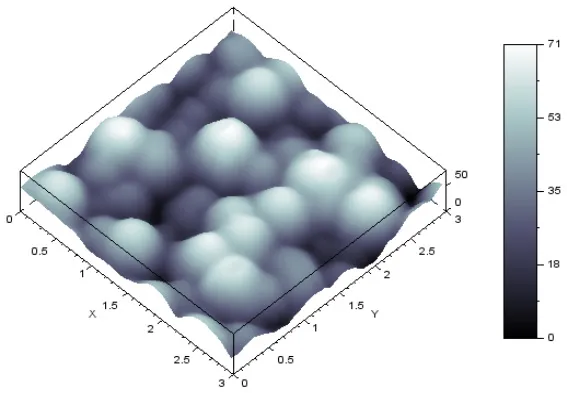 |
| Sa | 37.90 nm | Sa | 37.93 nm | ||
| Sq | 14.24 nm | Sq | 14.26 nm | ||
| Ssk | 0.12 | Ssk | 0.13 | ||
| Squ | 2.21 | Squ | 2.21 | ||
| Δz | 30 nm | 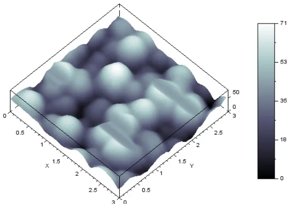 | Δz | 30 nm |  |
| Sa | 37.00 nm | Sa | 36.80 nm | ||
| Sq | 13.30 nm | Sq | 13.01 nm | ||
| Ssk | 0.08 | Ssk | 0.04 | ||
| Squ | 2.40 | Squ | 2.39 | ||
| Δz | 50 nm | 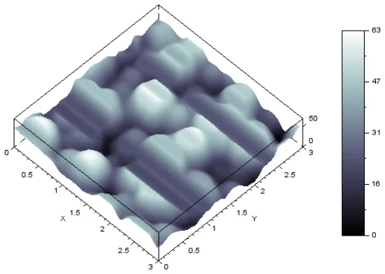 | Δz | 50 nm | 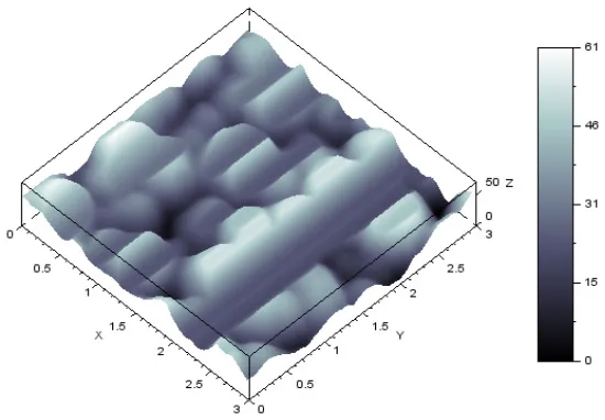 |
| Sa | 32.77 nm | Sa | 31.18 nm | ||
| Sq | 11.62 nm | Sq | 10.51 nm | ||
| Ssk | 0.29 | Ssk | 0.41 | ||
| Squ | 2.32 | Squ | 2.68 | ||
| Δz | 70 nm | 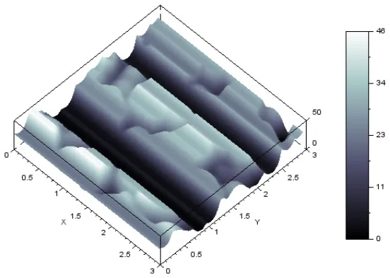 | Δz | 70 nm | 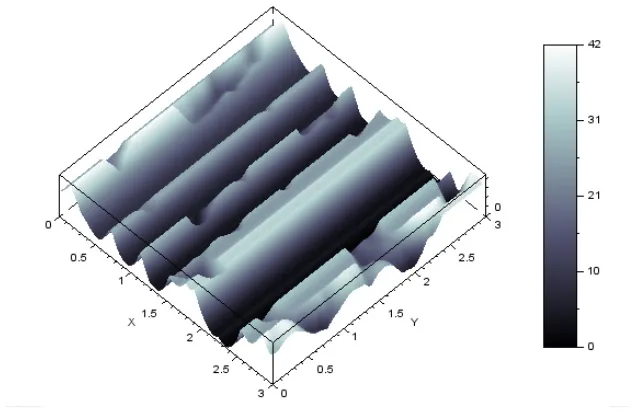 |
| Sa | 21.29 nm | Sa | 17.95 nm | ||
| Sq | 11.46 nm | Sq | 10.62 nm | ||
| Ssk | −0.27 | Ssk | 0.17 | ||
| Squ | 2.02 | Squ | 1.86 | ||
| Δz | 90 nm | 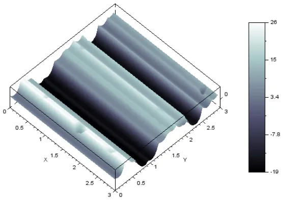 | Δz | 90 nm | 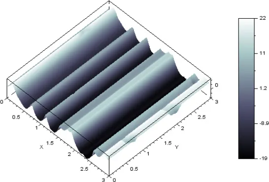 |
| Sa | 22.23 nm | Sa | 18.68 nm | ||
| Sq | 12.19 nm | Sq | 11.73 nm | ||
| Ssk | −0.41 | Ssk | 0.05 | ||
| Squ | 2.08 | Squ | 1.71 | ||
Simulated sliding wear surfaces illustarting transition in surface texture in both perpendicular X and Y directions.
The corresponding surface parametrs are given at the left side of each surface image.
Simulation result shows that at the vertical displacement of 10 nm there are no evident damages and surface has a random granular texture. When Δz reaches the range of 30–50 nm, the partial damages of spherical-like asperities occur with a lay direction along to the direction of sliding. The grooved texture becomes manifested at Δz of 70 nm and new grooved texture is completely formed at the displacement of 90 nm.
Comparing the images at the displacement of 90 nm one can conclude that the groove widths and their heights vary and the worn surfaces do not have a uniform groove profile in directions X and Y. Thus, the selected surface, shown in Figure 1, generates the dissimilar worn surfaces in perpendicular sliding directions X and Y. The resulting surface profiles are inverse to the effective surface profiles in corresponding direction as it presented in Figure 3. The location of asperity involved in the destructive friction process can be easily identified on the ESP graph in the selected direction of sliding.
Figure 3
Evolution of Roughness Parameters During the Simulated Abrasive Wear
To investigate, how the roughness parameters vary due to the transition of surface texture, a series of numerical calculations were performed by using the simulated worn surfaces described in previous section. All the calculations of roughness parameters were performed under the stepwise displacement control. A displacement Δz is set in the normal direction to the nominal plane of rough surface. The maximum value of Δz was set to 110 nm based on estimation result presented in previous section and was subdivided into 110 steps. The evolution of Sa and Sq of surface was investigated for a series of increasing displacement Δz and it is shown in Figure 4.
Figure 4
Several important observations can be done from Sa and Sq graphs (see Figure 3). Both of them begins from the corresponding values of surface Sa = 37.94 and Sq = 14.31, respectively. Graph of Sa consist of two parts. First part is characterized by gradual decreasing because the areas undergoing wear contribute to the overall decreasing of surface heights. However, at the vertical displacement Δz about 70 nm, Sa becomes to increase gradually and reach constant value of 22.25 and 18.76 in X and Y directions, respectively. It can be explained as following. At this displacement, the height magnitude of grooved structure becomes to dominate upon the initial granular structure, and stabilizes as a constant value when a worn grooved surface has finally formed. The drop on both graphs can be represented as a delimiter for an amplitude transition between virgin and worn surfaces.
In contrast to Sa, a graph of Sq has no sharp drop (see Figure 3B). Sq graph depicts as an inverted smoothed bell-like function with a minimum of Δz about 60 nm. Comparing to the transition behavior of Sa, Sq has reached the minimum value of Δz earlier than Sa. It means that Sq is more sensitive to the surface structure changes due to wear. Simulation result also shows that Sq tends to decrease at the initial stage of wear, where the upper parts of asperities underwent a minor material loss. The formation of grooved surface began to dominate, as the main surface texture, approximately at the minimum of Sq (see Table 1). Obtained results are in agreement with results of Jeng and co-authors (Jeng and Gao, 2000; Jeng et al., 2004), but represent more complicated transition behavior of Sa and Sq when the virgin surface is transformed to the grooved worn surface.
Figure 4 shows the evolution of Ssk and Sku during the transition of surface structures. The shape of curves has more complex behavior than shape of Sa and Sq. The results show that both skewness and kurtosis curves have peaks at Δz about 50 and 40 nm, respectively. Comparing the extreme points on the graphs of Sa, Sq, Ssk, Sku, one can conclude that a kurtosis (Sku) is more sensitive to the surface transformation due to wear.
Comparison between the roughness parameters of surface and its ESP profiles allows concluding that there are no evident matches. The values of Sa and Sq of the ESP are lower than those of Sa and Sq of the surface listed in Table 1. It is reasonable because the height range of ESP is up to twice lower than the average height range of surface profiles. Skewness and kurtosis (Ssk and Sku) cannot be qualitatively compared because the ESP profiles have the positive value of Ssk and Sku lower than 3 due to their origin always. The roughness parameters of ESPs and simulated worn surfaces are listed in Table 2.
Table 2
| Sa | Sq | Ssk | Sku | |
|---|---|---|---|---|
| ESP along X | 10.15 | 12.26 | 0.40 | 2.05 |
| ESP along Y | 10.55 | 11.89 | 0.07 | 1.69 |
| Worn surface along X | 10.15 | 12.21 | −0.40 | 2.08 |
| Worn surface along Y | 10.55 | 11.84 | −0.07 | 1.72 |
The roughness parameters of the effective surface profiles along axis X and Y, and corresponding worn surfaces.
Also, it should be noted, that presented graphs demonstrate a transition process occurring between two different surface structures, but final surface structure and its surface parameters could be predicted by the ESP in the selected direction.
As one would expect, the roughness parameters are similar for an effective surface profile and corresponding worn surfaces. The similarity presents because the ESP and corresponding worn surface are inverted in origin and the amplitude (height) roughness parameters are considered. The negative value of skewness is easily explained. The effective surface profile in most of cases will have the positive Ssk because it consists of rounded top asperities and sharp thin pits formed due to the overlapping of neighboring ones. The worn surface has an inverted structure: the thin sharp peaks and big curved valleys that characterizes by the negative skewness. A small variation in the values of Sq and Sku are probably caused by the digitizing collapsing error in calculation procedure implemented, which is different for an inverted data profiles.
Thus, the main feature of the roughness parameters of ESP and worn surfaces, listed in Table 2, is that these parameters were evaluated based on the height data of real surface with implementation of concept of the effective surface profile, presented in Figure 2, and allow qualitative prediction of the structure of worn surface and its roughness parameters.
Conclusions
A new consideration of conventional surface data has been presented to predict the structure of worn profile that could be formed during abrasive wear process. Such consideration allows us to introduce the concept of an effective surface profile as a powerful phenomenological tool for surface characterization based on the height data of initial rough surface. The wear process, discussed in this paper, is considered as the degradation of the soft rough surface by the interlocking hard irregularities, plowing, and abrasion of material by means of the hard asperities of counterface rather than adhesion of asperities in friction and without consideration of cases in which wear debris are trapped onto the contact area.
The results of roughness analysis of profiles, which were derived from rough surface, have clearly shown that, in the present case, there is no good correlation of the height roughness parameters Sa, Sq, Sku, Ssk of the surface topography with the corresponding parameters of surface profiles. It was deduced that this approach is not effective for the prediction of worn surface structure formed during sliding friction.
The concept of effective surface profile has been proposed to construct the front profile of surface consisting of asperities involved in the contact during sliding friction.
In the frame of idealized model of sliding of a hard rough surface upon a soft rough one, the contact area As and contact pressure Ps, under the shakedown pressure ps, were theoretically estimated.
A simulation procedure is proposed for topographical representation of worn surfaces produced by the rough surface in both perpendicular directions. The effective surface profiles as a template of possible transformation of soft surface are used in selected directions. The roughness parameters of worn surfaces are estimated and compared. It has been revealed that the prediction of worn surface structure and its roughness parameters are possible by using effective surface profile with respect to the selected direction of sliding.
The results above widen the understanding of friction and will advance the ability to predict the wear pattern on a surface that has not been attended before in the surface analysis in tribology.
Statements
Author contributions
AK proposed the concept of effective surface profile and done calculations. ZY and CH conducted measurements. YM involved in the preparation of the manuscript.
Acknowledgments
This work was supported by the National Natural Science Foundation of China (NSFC) with grant No. 51635009 and the Tsinghua University Initiative Scientific Research Program No.2015THZ0.
Conflict of interest
The authors declare that the research was conducted in the absence of any commercial or financial relationships that could be construed as a potential conflict of interest.
References
1
AdamsG. G.NosonovskyM. (2000). Contact modeling — forces. Tribol. Int. 33, 431–442. 10.1016/S0301-679X(00)00063-3
2
AoY.WangQ. J.ChenP. (2002). Simulating the worn surface in a wear process. Wear252, 37–47. 10.1016/S0043-1648(01)00841-9
3
ArchardJ. F. (1953). Contact and rubbing of flat surfaces. J. Appl. Phys. 24, 981–988. 10.1063/1.1721448
4
AslanD.BudakE. (2015). Surface roughness and thermo-mechanical force modeling for grinding operations with regular and circumferentially grooved wheels. J. Mater. Process. Technol. 223, 75–90. 10.1016/j.jmatprotec.2015.03.023
5
BhushanB. (1998). Contact mechanics of rough surfaces in tribology: multiple asperity contact. Tribol. Lett. 4, 1–35. 10.1023/A:1019186601445
6
BhushanB. (2001). Chapter 2: Surface roughness analysis and measurement techniques, in Modern tribology handbook. Vol. 1, ed BhushanB. (Boca Raton, FL: CRC Press), 49–119. 10.1201/9780849377877.ch2
7
BorodichF. M.BianchiD.Surface synthesis based on surface statistics, in Encyclopedia of Tribology, eds WangQ. J.ChungY.-W. (Boston, MA: Springer), 3472–3478. 10.1007/978-0-387-92897-5_309
8
BorodichF. M.PepelyshevA.SavencuO. (2016). Statistical approaches to description of rough engineering surfaces at nano and microscales. Tribol. Int. 103, 197–207. 10.1016/j.triboint.2016.06.043
9
BorodichF. M.SavencuO. (2017). Hierarchical models of engineering rough surfaces and bio-inspired adhesives, in Bio-Inspired Structured Adhesives, eds. HeepeL.XueL.GorbS. N. (Cham: Springer), 179–219. 10.1007/978-3-319-59114-8_10
10
BowdenF. P.TaborD. (1964). Friction and Lubrication of Solids. Oxford: Clarendon Press.
11
CabanettesF.RosénB.-G. (2014). Topography changes observation during running-in of rolling contacts. Wear315, 78–86. 10.1016/j.wear.2014.04.009
12
CaoY.GuanJ.LiB.ChenX.YangJ.GanC. (2013). Modeling and simulation of grinding surface topography considering wheel vibration. Int. J. Adv. Manuf. Technol.66, 937–945. 10.1007/s00170-012-4378-7
13
ChallenJ. M.McLeanL. J.OxleyP. L. B. (1984). Plastic deformation of a metal surface in sliding contact with a hard wedge: its relation to friction and wear. Proc. R. Soc. London A Math. Phys. Eng. Sci. 394, 161–181. 10.1098/rspa.1984.0074
14
da SilvaW. M.de MelloJ. D. B. (2009). Using parallel scratches to simulate abrasive wear. Wear267, 1987–1997. 10.1016/j.wear.2009.06.005
15
DarafonA.WarkentinA.BauerR. (2013). 3D metal removal simulation to determine uncut chip thickness, contact length, and surface finish in grinding. Int. J. Adv. Manuf. Technol. 66, 1715–1724. 10.1007/s00170-012-4452-1
16
DongW.SullivanP.StoutK. (1992). Comprehensive study of parameters for characterizing three-dimensional surface topography I: some inherent properties of parameter variation. Wear159, 161–171. 10.1016/0043-1648(92)90299-N
17
DongW.SullivanP.StoutK. (1993). Comprehensive study of parameters for characterizing three-dimensional surface topography II: statistical properties of parameter variation. Wear167, 9–21. 10.1016/0043-1648(93)90050-V
18
DongW.SullivanP.StoutK. (1994a). Comprehensive study of parameters for characterising three- dimensional surface topographyIII: parameters for characterising amplitude and some functional properties. Wear178, 29–43. 10.1016/0043-1648(94)90127-9
19
DongW.SullivanP.StoutK. (1994b). Comprehensive study of parameters for characterising three-dimensional surface topographyIV: parameters for characterising spatial and hybrid properties. Wear178, 45–60. 10.1016/0043-1648(94)90128-7
20
EldredgeK. R.TaborD. (1955). The mechanism of rolling friction. I. The plastic range. Proc. R. Soc. A Math. Phys. Eng. Sci.229, 181–198. 10.1098/rspa.1955.0081
21
EtsionI. (2012). Discussion of the paper: optical in situ micro tribometer for analysis of real contact area for contact mechanics, adhesion, and sliding experiments. Tribol. Lett. 46, 205–205. 10.1007/s11249-012-9930-y
22
GadelmawlaE. S.KouraM. M.MaksoudT. M. A.ElewaI. M.SolimanH. H. (2002). Roughness parameters. J. Mater. Process. Technol. 123, 133–145. 10.1016/S0924-0136(02)00060-2
23
GlaeserW. A. (1992). Materials for Tribology. Amsterdam: Elsevier Science.
24
GongY.WangB.WangW. (2002). The simulation of grinding wheels and ground surface roughness based on virtual reality technology. J. Mater. Process. Technol. 129, 123–126. 10.1016/S0924-0136(02)00589-7
25
GoryachevaI. G. (1998). Contact Mechanics in Tribology. Dordrecht: Kluwer Academic Pablishers.
26
GreenwoodJ. A. (1997). Analysis of elliptical Hertzian contacts. Tribol. Int.30, 235–237. 10.1016/S0301-679X(96)00051-5
27
GreenwoodJ. A.WilliamsonJ. B. P. (1966). Contact of nominally flat surfaces. Proc. R. Soc. Lond. A. Math. Phys. Sci. 295, 300–319. 10.1098/rspa.1966.0242
28
GreenwoodJ. A.WuJ. J. (2001). Surface roughness and contact: an apology. Meccanica. 36, 617–630. 10.1023/A:1016340601964
29
HaoL.MengY. (2015). Numerical prediction of wear process of an initial line contact in mixed lubrication conditions. Tribol. Lett. 60:31. 10.1007/s11249-015-0609-z
30
HaywardI. P.SingerI. L.SeitzmanL. E. (1992). Effect of roughness on the friction of diamond on cvd diamond coatings. Wear157, 215–227. 10.1016/0043-1648(92)90063-E
31
HsuS. M.ShenM. C.RuffA. W. (1997). Wear prediction for metals. Tribol. Int. 30, 377–383. 10.1016/S0301-679X(96)00067-9
32
JengY.-R.GaoC.-C. (2000). Changes of surface topography during wear for surfaces with different height distributions. Tribol. Trans. 43, 749–757. 10.1080/10402000008982404
33
JengY.-R.LinZ.-W.ShyuS.-H. (2004). Changes of surface topography during running-in process. J. Tribol. 126, 620–625. 10.1115/1.1759344
34
JiangX.ScottP. J.WhitehouseD. J.BluntL. (2007a). Paradigm shifts in surface metrology. Part I. Historical philosophy. Proc. R. Soc. A Math. Phys. Eng. Sci. 463, 2049–2070. 10.1098/rspa.2007.1874
35
JiangX.ScottP. J.WhitehouseD. J.BluntL. (2007b). Paradigm shifts in surface metrology. Part II. The current shift. Proc. R. Soc. A Math. Phys. Eng. Sci. 463, 2071–2099. 10.1098/rspa.2007.1873
36
KapoorA.JohnsonK. L. (1992). Effect of changes in contact geometry on shakedown of surfaces in rolling/sliding contact. Int. J. Mech. Sci. 34, 223–239. 10.1016/0020-7403(92)90073-P
37
KapoorA.JohnsonK. L. (1994). Plastic ratchetting as a mechanism of metallic wear. Proc. R. Soc. A Math. Phys. Eng. Sci.445, 367–384. 10.1098/rspa.1994.0066
38
KapoorA.WilliamsJ. A.JohnsonK. L. (1994). The steady state sliding of rough surfaces. Wear175, 81–92. 10.1016/0043-1648(94)90171-6
39
KatoK. (2002). Classification of wear mechanisms/models. Proc. Inst. Mech. Eng. Part J J. Eng. Tribol. 216, 349–355. 10.1243/09544110260216649
40
LuW.ZhangG.LiuX.ZhouL.ChenL.JiangX. (2014). Prediction of surface topography at the end of sliding running-in wear based on areal surface parameters. Tribol. Trans. 57, 553–560. 10.1080/10402004.2014.887165
41
ManierC.-A.SpaltmannD.TheilerG.WoydtM. (2008). Carboneous coatings by rolling with 10% slip under mixed/boundary lubrication and high initial Hertzian contact pressures. Diam. Relat. Mater. 17, 1751–1754. 10.1016/j.diamond.2008.01.066
42
MengH. C.LudemaK. C. (1995). Wear models and predictive equations: their form and content. Wear 181–183, 443–457. 10.1016/0043-1648(95)90158-2
43
PopovV. (2010). Contact Mechanics and Friction - Physical Principles and Applications. Berlin: Springer-Verlag.10.1007/978-3-642-10803-7
44
PopovV. L.PohrtR. (2018). Adhesive wear and particle emission: numerical approach based on asperity-free formulation of Rabinowicz criterion. Friction6, 260–273. 10.1007/s40544-018-0236-4
45
ReizerR.PawlusP.GaldaL.GrabonW.DzierwaA. (2012). Modeling of worn surface topography formed in a low wear process. Wear 278–279, 94–100. 10.1016/j.wear.2011.12.012
46
SepJ.TomczewskiL.GaldaL.DzierwaA. (2017). The study on abrasive wear of grooved journal bearings. Wear 376–377, 54–62. 10.1016/j.wear.2017.02.034
47
ShahabiH. H.RatnamM. M. (2016). Simulation and measurement of surface roughness via grey scale image of tool in finish turning. Precis. Eng. 43, 146–153. 10.1016/j.precisioneng.2015.07.004
48
StoutK. J. (1993). The Development of Methods for the Characterisation of Roughness in Three Dimentions, 1st Edn. Birmingham: University of Birmingham Edgbaston.
49
XieY.WilliamsJ. A. (1996). The prediction of friction and wear when a soft surface slides against a harder rough surface. Wear196, 21–34. 10.1016/0043-1648(95)06830-9
50
YuC.WangQ. J. (2012). Friction anisotropy with respect to topographic orientation. Sci. Rep. 2:988. 10.1038/srep00988
51
YuanC. Q.PengZ.YanX. P.ZhouX. C. (2008). Surface roughness evolutions in sliding wear process. Wear265, 341–348. 10.1016/j.wear.2007.11.002
52
YuanC. Q.YanX. P.PengZ. (2007). Prediction of surface features of wear components based on surface characteristics of wear debris. Wear263, 1513–1517. 10.1016/j.wear.2006.11.029
53
ZhuravlevV. A. (2007). On the question of theoretical justification of the Amontons—Coulomb law for friction of unlubricated surfaces. Proc. Inst. Mech. Eng. Part J J. Eng. Tribol. 221, 893–898. 10.1243/13506501JET176
54
ZmitrowiczA. (2006). Wear patterns and laws of wear – a review. J. Theor. Appl. Mech. 44, 219–253. Available online at: http://www.ptmts.org.pl/jtam/index.php/jtam/article/view/v44n2p219/469
Summary
Keywords
sliding wear, plowing, abrasion, surface topography, surface parameters
Citation
Kovalev A, Yazhao Z, Hui C and Meng Y (2019) A Concept of the Effective Surface Profile to Predict the Roughness Parameters of Worn Surface. Front. Mech. Eng. 5:31. doi: 10.3389/fmech.2019.00031
Received
11 December 2018
Accepted
17 May 2019
Published
06 June 2019
Volume
5 - 2019
Edited by
Roman Pohrt, Technische Universität Berlin, Germany
Reviewed by
Árpád Czifra, Óbuda University, Hungary; Ivan Y. Tsukanov, Institute for Problems in Mechanics (RAS), Russia
Updates
Copyright
© 2019 Kovalev, Yazhao, Hui and Meng.
This is an open-access article distributed under the terms of the Creative Commons Attribution License (CC BY). The use, distribution or reproduction in other forums is permitted, provided the original author(s) and the copyright owner(s) are credited and that the original publication in this journal is cited, in accordance with accepted academic practice. No use, distribution or reproduction is permitted which does not comply with these terms.
*Correspondence: Yonggang Meng mengyg@tsinghua.edu.cn
This article was submitted to Tribology, a section of the journal Frontiers in Mechanical Engineering
Disclaimer
All claims expressed in this article are solely those of the authors and do not necessarily represent those of their affiliated organizations, or those of the publisher, the editors and the reviewers. Any product that may be evaluated in this article or claim that may be made by its manufacturer is not guaranteed or endorsed by the publisher.