On the Use of Semi-empirical Flame Models for Spreading Chaparral Crown Fire

Introduction

The occurrence of large fires has increased significantly in many regions around the world. One region particularly impacted by wildfires is southern California, where the terrain, highly flammable fuels, dry ambient conditions and fast foehn type winds (known locally as Santa Ana winds) generate conditions highly favorable to wildfire (Rothermel and Philpot, 1973). Thus, fuel and weather conditions exist such that in the event of an ignition event, the potential for wildfire is high. In the southern California case, growing wildfire potential, and fast population growth have occurred in parallel. This coupled growth has prompted changes to the so-called wildland urban interface, that is, the region separating the wildland from urban settlements. The growth of the wildland urban interface coupled with increased fire risk, places people and their property closer to fire. Because of the growing threat, the ability to accurately predict fire behavior has become paramount. This is contingent on thorough understanding of physical mechanisms driving fire spread and intensity. Because wildfire behavior is shaped by its environment, it is important to define the key conditions shaping fire behavior in a regional landscape and climate. In mediterranean climates, chaparral fires typically burn as crown fires (Barro and Conard, 1991), a category of fire consisting of two fuel layers, an above ground surface fuel layer and an elevated fuel layer known as a crown layer. In chaparral crown fires, fires typically start in the easily ignitable surface fuels and spread in the crown fuel layer (Tachajapong et al., 2014). Before a fire can spread in the crown, the fire must move vertically from the surface fuels to ignite crown fuels, a process defined as transition (Weise et al., 2018a).

Little is known of the exact mechanisms which produce effective transition and spread in chaparral crown fires. Transition and spread in crown fire, involves a dynamic energy exchange between the surface and crown fuel layers. Spread in the crown fuel layer may require energy to be supplied from the surface fuel layer, as in passive or dependent crown fires; or may rely on the crown fuel layer alone to maintain successful spread, as in independent fires (Van Wagner, 1977). In the case of crown fire spread where energy is partially or solely supplied by the crown fuel layer, identifying the mechanism through which energy is exchanged from the crown flame to unburned fuel is necessary to better understand mechanisms for successful crown fire spread. Hence, assessing flame properties in the crown fuel layer, particularly flame geometry, may be a key step in generating a rigorous characterization of chaparral crown fire behavior.

Flame geometry has been shown to influence flame spread through radiative heat transfer (Albini, 1985). Thus, numerous groups have focused on assessing flame geometry properties as they relate to fire spread. It is pertinent then to present a brief review of studies examining flame geometry characteristics for wildland fuels; this now follows. Byram (1959) conducted foundational work to characterize combustion and fire behavior in forest fuels. The Byram intensity which defines heat release rate per unit time per unit length, is perhaps the most widely accepted expression for fire intensity. Byram proposed early correlations relating flame length to fire intensity. Since the first formulation, numerous groups have derived semi-empirical expression of flame length as a function of fire intensity for various fuels. Thomas proposed correlations relating flame height to fuel supply rate and burner dimensions in conditions without wind (Thomas et al., 1961) and with wind (Thomas, 1963). In work by Nelson (1980) theoretical formulations for flame length, height, tip velocity and tilt angle as a function of Byram intensity were examined for light southern pine fuels. In addition to theoretical modeling, the work presents results from semi-empirical power-law modeling of flame length and tip velocity as a function of Byram intensity. Steward (1970) derived mathematical expressions relating mass flow rate to flame height. Zukoski et al. (1980) examined entrainment characteristics in methane diffusion flames and proposed power-law correlations of flame height as a function of heat release rate and burner diameter. Similarly, Heskestad (1983, 1984) related flame height to heat release rate and burner diameter. Other recent studies of flame conditions and flame spread include those by Gang et al. (2017) and Zhou et al. (2018). Fernandes et al. (2009) derived empirical correlations of flame length and flame height for head and back wildfires. They expressed flame length and height of head fires as a function of Byram intensity and fuel loading. For back fires, both flame length and height were expressed as a function of Byram intensity. Alexander and Cruz (2012) surveyed expressions of flame length presented as function of fire intensity. Alexander and Cruz (2012) identify the significance of flame length to crown fuel layer ignition behavior and highlight power-law expressions relating Byram intensity to flame length for various fuels. Fernandes et al. (2000) derived a powerlaw expression relating Byram intensity for flame length in shrublands. Other recent studies of flame spread include those by Gang et al. (2017) and Zhou et al. (2018).

Works focusing on flame geometry for shrub and chaparral fuels include computational evaluation of flame properties such as the one by Padhi et al. (2016) in which flame geometry in a stationary shrub fire was considered. Moreover, a numerical analysis of flame tilt angle and height, in a spreading shrub fire was presented by Morvan (2007). Recent work by Weise et al. (2018b) compared predictions from flame models to results from experimental circular and line fire configurations of chaparral fire. Model predictions of flame height and flame tilt angle, were compared against experimental values in work by Nelson et al. (2012). Laboratory scale work by Weise and Biging (1996) evaluated the effect of wind and slope on flame properties. Importantly, the previous experimental studies did not include a dual layer, crown fire configuration.

Results from the works reviewed above include semi-empirical correlations which show promise in predicting fire spread behavior. However, few of these semi-empirical models have been produced through the study of chaparral fire modeled as crown fire, as done when modeling chaparral fire with distinct fuel layers for surface and crown fuels. Thus, the aim here is to examine crown flame geometry and to survey the applicability of semi-empirical models of flame geometry to chaparral fires modeled as dual-layer crown fires. To the knowledge of the authors, no prior work has attempted to use established models of semi-empirical fire spread for chaparral fuels modeled with distinct layers for the surface and crown fuel beds. We consider that modeling chaparral fires with a dual layer configuration will more precisely replicate spread behavior as it can capture the dynamic energy exchange between the surface and crown fires. To this purpose, this paper compares models of flame geometry to observations of flame data obtained from wind tunnel experiments in which the surface and crown fuel beds were modeled as separate fuel beds. Data from experiments with wind-blown spread are examined. The next section describes the experimental procedure and modeling approach.

Methodology

Experimental

Experiments were conducted in a specialized wind tunnel located at the USDA Forest Service Pacific Southwest Research Station fire laboratory in Riverside, California. The wind tunnel study area was composed of two distinct fuel beds representing the dead fuel surface layer and the live fuel crown layer. The surface fuel layer was constructed on the wind tunnel floor and a platform mounted on the top of the tunnel frame contained the crown fuel bed (see Figure 1). Aspen (Populus tremuloides Michx.) excelsior (shredded wood) served as the surface fuel; crown fuels consisted of chamise (Adenostoma fasciculatum Hook & Arn.) branches and foliage harvested locally. Custom instrumentation was developed to measure mass loss from the crown fuel layer; full details of this system can be found in Cobian-Iñiguez et al. (2017). Surface fuel mass loss was measured using an electronic scale placed under a portion of the excelsior fuel bed. Fires were started by igniting the surface fuel bed (excelsior) using a butane torch and ethyl alcohol as lighter fluid. Wind was activated simultaneously with surface fuel bed ignition. Once ignited, the excelsior fuel bed developed a flame and the fire spread. The surface fire spread under the crown fuel thus preheating it to the point of ignition, at this point the fire transitioned to the crown fuel layer. Thereafter, a flame developed in the crown fuel layer and the fire in the crown fuel layer was allowed to spread until extinction.

FIGURE 1

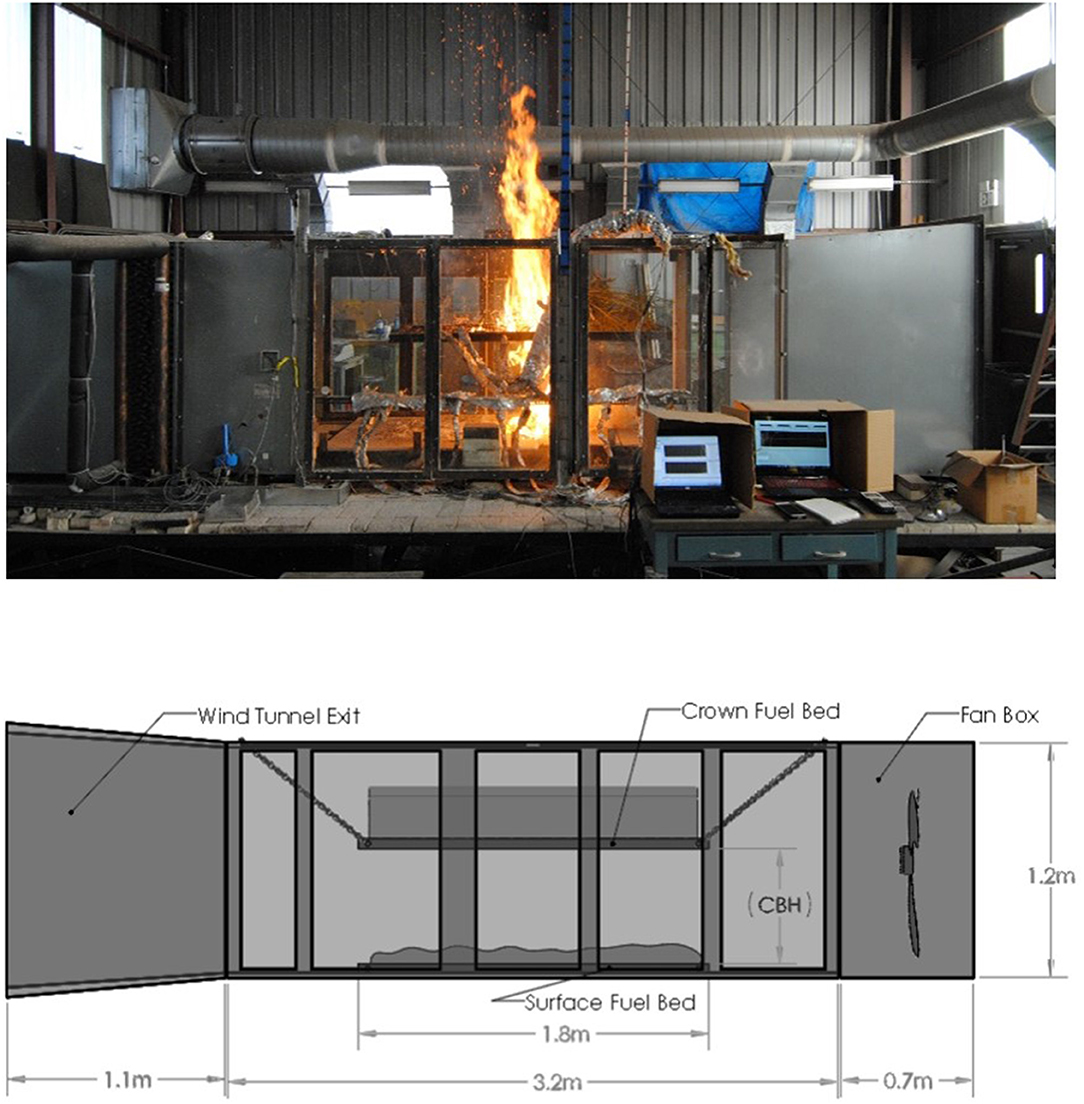
Figure 1. Photograph with wind tunnel configuration with crown base height (CBH), flame height (H) and experimental configuration labels (top). Schematic of wind tunnel with major dimensions labeled (bottom).

Before explaining the properties that were measured using the image processing techniques here, it is necessary to note some basics of flame geometry. In microgravity, experiments have shown and demonstrated that a laminar diffusive flame has a spherical shape. When gravity is applied, a good approximation is to assume that gravity forces will stretch the spherical shape of the flame like a candle and the resulting shape will be an ellipsoidal. Following the same logic, when analyzing the shape of a turbulent diffusive flame, an ellipsoidal (in the case of 2D projection, an ellipse) can be used as a reference for flame characteristics such as flame length and flame tilt.

Flame geometry was obtained from video recordings obtained using a Sony Handicam¹ at 30 frames per s. We used two different algorithms for video data processing: one for flame height, H, see Figure 1, and another one for flame tilt angle, θ_f, and flame length, L_f, see Figure 2F. The flame height algorithm was generated in MATLAB. The script was designed to convert raw red-green-blue (RGB) images to black and white images through thresholding in order to isolate the flame and generate a flame perimeter image. Flame height was obtained from the flame perimeter image. Video data was resampled from 30 to 1 Hz. Once the datum were re-sampled, flame height was obtained at 1 s intervals. The resulting data were used to obtain one absolute maximum flame height value for each experiment. The complete flame height dataset included both the surface and crown flame. Therefore, for the purposes of the analysis shown here, the surface flame height was cropped out. Computationally, this was done by identifying the vertical location of the crown fuel bed in a sample image of the experimental setup. The pixel value at this location was extracted and selected as a threshold. A script was developed to filter out values falling under the threshold thus isolating the crown fuel bed.

FIGURE 2

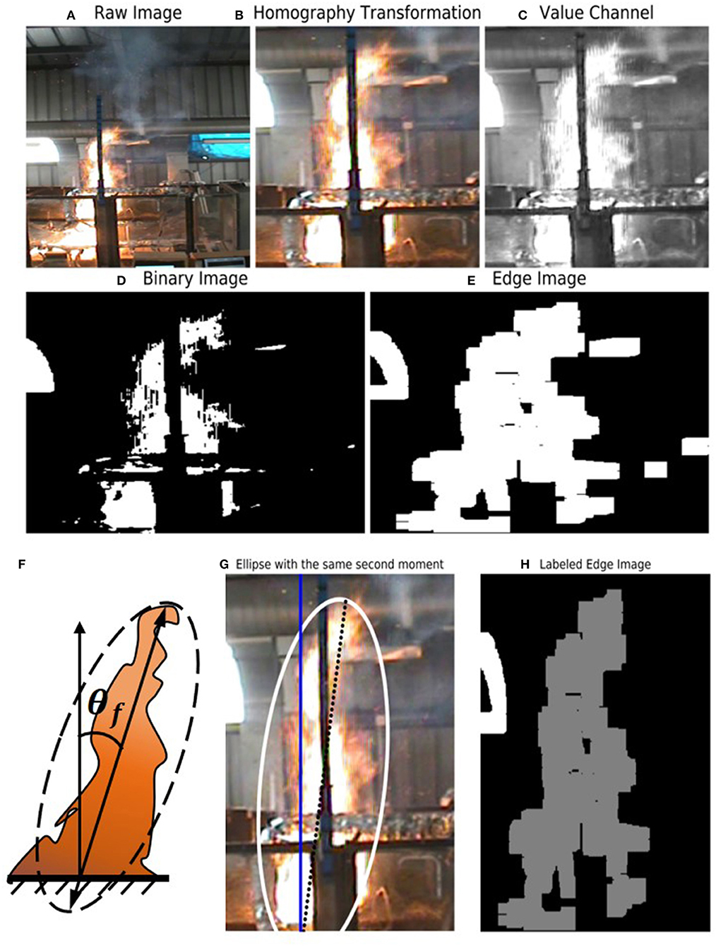
Figure 2. Flame tilt computer vision algorithm image processing steps and schematic (clockwise from the leftmost top corner): (A) raw image (B) homographic transformation (C) value channel extraction (D) binary image (E) edge image (H) labeled edge image (G) ellipsoid generated from the processed image overlapped in RGB raw image (F) schematic with flame length and flame tilt angle labeled.

An algorithm based on computer vision was developed to obtain flame tilt angle and flame length from an experiment video. The use of this methodology is motivated by advancements in computer vision over the past decade through which image processing for fire imaging has improved. Edge detection has been used to identify flame edge contours (e.g. Gupta and Gaidhane, 2014). The fundamental parameters that can be obtained from visual images are flame height, flame tilt, and flame length. The algorithm and process used here to obtain such parameters follow. At first, images were preprocessed to obtain edges of the flame. To do so, first, a homography and prospective transformation was applied to the raw image. The transformation corrected the perspective of the images. Later, the RGB channeled image was converted to hue-saturation-value images (HSV) format and the value channel (V) was extracted from the image. Subsequently, a threshold value was selected to convert the images to a binary image. Once the image was converted to binary, the flame edge, or perimeter was obtained using an edge detection algorithm, Sobel edge detection.

After obtaining the flame edge, the binary or edge images (Figures 2D,E) were labeled and segmented into discrete flames (Figure 2F) (in case of both surface and crown fuel flames) distinct from each other and the background. This step essentially established what were known in image processing as regions. The regions, the crown flame and surface flame, region 1, and region 2, were now the computational objects of interest. Once the regions were established, the image features, flame length and orientation, were computed. This was done by calculating the moments of the region as described by Burger and Burge (2008). Calculations of the second moment returned orientation and major axis of the region. The coordinates and dimensions of the major axis and orientation were used to produce an ellipsoid using the OpenCV (Bradski, 2000) library in Python. This produced an ellipsoid which enveloped the flame and had a major axis equal to the flame length and an orientation equal to the flame tilt angle. The last processing step leading up to the generation of the ellipsoid was visualized in Figure 2G. For the purposes of the study here, only region 1, the crown flame was analyzed.

Modeling Techniques

Data obtained experimentally was compared to predictions from existing semi-empirical models to be described in this section. The goal was to assess whether currently available models accurately describe the chaparral crown fire system modeled. Flame geometry properties were defined according to naming and measuring conventions described by Figures 1, 2. Predicted flame height was calculated from heat release rate (Q). Theoretical heat release rate was obtained from mass loss rate according to Equation (1)

$\begin{array}{ll}\begin{array}{c}\dot{Q}=h\left(\frac{dm}{dt}\right),\end{array}& (1)\end{array}$

where h represented the low heat of combustion (for chamise h = 14.71 KJ/g). Following Zukoski et al. (1980), we modeled flame height using a semi-empirical power-law correlation of the forms in Equations 2 and 3,

$\begin{array}{ll}\begin{array}{c}{H}_{max}=0.2{\dot{Q}}_{max}^{\frac{2}{5}},\end{array}& (2)\end{array}$

where H_max and ${\dot{Q}}_{max}$ represented maximum flame height and maximum heat release rate, respectively. The second approach was to use the power-law correlation proposed by Sun et al. (2006)

$\begin{array}{ll}\begin{array}{c}{H}_{max}=0.17{\dot{Q}}_{max}^{0.43}.\end{array}& (3)\end{array}$

We obtained maximum heat release rate using the two methods proposed by Sun et al. (2006) which, for consistency, we name following their convention such that in Method 1, maximum heat release rate was defined as the heat loss rate occurring at the time of maximum mass loss rate (${\dot{Q}}_{max,Method1}~\dot{m}(t_{{\dot{m}}_{max}})$). In Method 2, maximum heat release rate was defined as the heat loss rate occurring at the time of maximum flame height ${\dot{Q}}_{max,Method2}~\dot{m}(t_{flameheight,max})$. In addition to flame height, we estimated flame tilt from power law and log-log correlations.

Next, we obtained predicted flame tilt values. Predicted flame tilt as a function of Froude number, a dimensionless measure of the relative importance of buoyant and inertial forces Williams (Williams, 1985), was compared to experimental data. The general form for Froude number is given by

$\begin{array}{ll}\begin{array}{c}Fr=\frac{U^2}{gD},\end{array}& (4)\end{array}$

where U is the gas velocity, g is the gravitational constant and D is the characteristic length (Drysdale, 2011). To correlate Froude number to flame tilt angle, some have used flame height, H, as a characteristic length (Albini, 1981) while others have used flame length, L_f, (Putnam, 1965). In the approach here the latter was used, hence the resulting Froude number expression used was of the final form given by Equation (5)

$\begin{array}{ll}\begin{array}{c}Fr=\frac{U^2}{g{L}_f}.\end{array}& (5)\end{array}$

The empirical correlation between flame tilt angle, θ_f, and Froude number, Fr, was of the form given by Equation (6) (Albini, 1981; Nelson and Adkins, 1986; Weise and Biging, 1996)

$\begin{array}{ll}\begin{array}{c}tan({\theta }_f)=\alpha F{r}^{\beta }.\end{array}& (6)\end{array}$

In Equation 5, θ_f is the flame tilt angle as measured from the vertical as presented in Figure 2B. The coefficient α and power dependence β can be estimated following the regression analysis in Weise and Biging (1996) (Figure 2F).

Coefficients to fit Equation (6) to the data from chaparral crown fire experiments were obtained through regression analysis.

Error Analysis

Agreement between the observed and predicted values of flame height and flame tilt was quantified using the measures identified in Cruz and Alexander (2013) and Weise et al. (2018b). These error analysis schemes have been previously used in analyzing results from wildland fire behavior studies (Cruz and Alexander, 2013). Perhaps the most elemental form of difference is simply the difference between observed and predicted values or

$\begin{array}{ll}\begin{array}{c}d=(P_i-O_i),\end{array}& (7)\end{array}$

where we have adopted notation from Willmott (1982) to represent observed values by O and predicted values by P. If N is the number of samples, then the mean bias of the error (MBE), the mean absolute error (MAE) and the root mean square error (RMSE) can be given as

$\begin{array}{ll}MBE=N^{-1}{\displaystyle {\sum }_{i=1}^N\left(P_i-O_i\right),}& (8)\end{array}$

$\begin{array}{ll}MAE=N^{-1}{\displaystyle {\sum }_{i=1}^N\left|P_i-O_i\right|,}& (9)\end{array}$

$\begin{array}{ll}\begin{array}{c}\begin{array}{c}RMSE={\left[N^{-1}{\displaystyle {\sum }_{i=1}^N{\left(P_i-O_i\right)}^2}\right]}^{0.5}.\end{array}\end{array}& (10)\end{array}$

Willmott (1982) qualified RMSE and MAE as the best measures of model performance and claimed that MBE is not a sufficient measure of error as it is simply an expression of the difference between mean values. Here we included RMSE and MAE as the primary measures of difference. MBE was used as a supplemental measure as it provided a sense of over prediction or under prediction of experimental results. Moreover, we calculated the normalized root mean square error (NRMSE) by normalizing RMSE with the mean of the observed values

In this way we aimed to provide RMSE as a percentage error. The mean absolute percent error (MAPE), Equation 12, was also measured and it provides an additional form of percentage error

$\begin{array}{ll}\begin{array}{c}NRMSE=\left(\frac{RMSE}{O}\right)·100.\end{array}& (11)\end{array}$

$\begin{array}{ll}\begin{array}{c}MAPE=N^{-1}\left[{\displaystyle {\sum }_{i=1}^N\left(\frac{P_i-O_i}{O_i}\right)}\right]·100.\end{array}& (12)\end{array}$

According to Cruz and Alexander (2013), percentage error as measured by MAPE is optimized as it nears zero and an acceptable range for good values is 10%.

Experiment Classification

Four experiment classes were used to quantify the effect of wind and the separation distance between the surface and crown fuel layer, which following Van Wagner (1977) is called crown base height (CBH) in this work. Table 1 summarizes the conditions for each experimental class.

TABLE 1

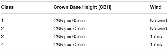
Table 1. Table of experiment classes.

The effect of wind and crown base height on flame height was examined for all experimental classes. A total of 18 experiments were considered for flame height analysis. Flame tilt was primarily observed in wind driven flame spread, experiment classes 1 and 2. For this stage of the study, we focused only on the effect of wind on flame tilt, therefore we focused only on one experimental class for the flame tilt analysis, class 4. Two experiments conducted on the same day were examined. This enabled greater uniformity in fuel conditions as fuels burned for both experiments were collected on the same day under the same ambient conditions. Experiment A (experiment burn time = 171 s, RH = 52%, FMC = 54%) was the first experiment analyzed, Experiment B (experiment burn time = 385 s, RH = 28%, FMC = 54%) was the second.

Results

Flame Height

Data from experiments with and without wind with two crown base height values (CBH₁ = 60 cm and CBH₂ = 70 cm) were considered for the analysis. Power law relationships as described by Equations (2) and (3) were used to estimate maximum flame heights from maximum heat release rates for each experiment. For flame height analysis, experiments from all classes were considered.

Comparison of the data with Equations (2) and (3) did not show significant differences between models which is not surprising (Figure 3). When comparing observed values to theoretical values using Method 1 to estimate maximum heat release rate (Figure 3A), it was observed that just under 70% of experiments were over-estimated by the model. Theoretical values estimated using method 2, over 75% of experiments considered were under-estimated (Figure 3B). Comparison of observed and predicted values showed that for Method 1, only 10% of experiments fell outside 70% of accuracy (Figure 4A). In the case of power law predictions using method 2, 17% of experiments fell outside the bounds of 70% of accuracy (Figure 4B).

FIGURE 3

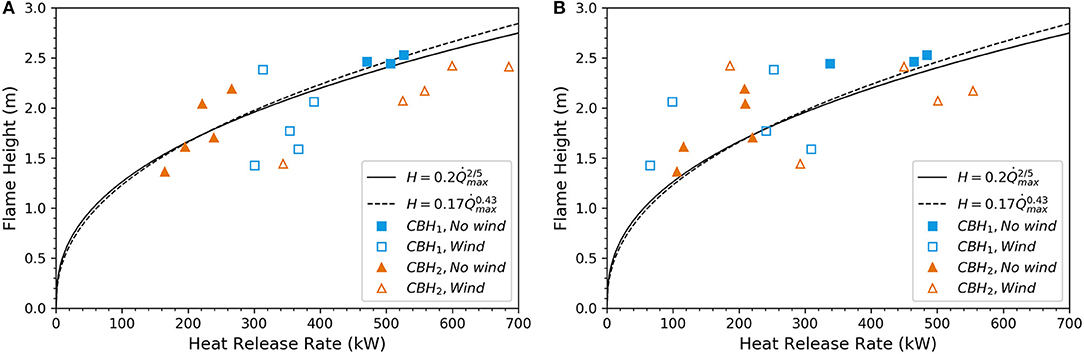
Figure 3. Maximum flame height per experiment as a function of heat release rate plotted against two-fifths power law and Sun et al. power law for chaparral fuels burned in fall season. Maximum heat flux estimated using: (A) Method 1, ${\dot{Q}}_{max}$ obtained from ṁ_max [${\dot{Q}}_{max,Method1}~\dot{m}(t_{{\dot{m}}_{max}})$]. (B) Method 2, ${\dot{Q}}_{max}$ obtained from $\dot{m}(t_{H_{max}}){\dot{Q}}_{max,Method2}~\dot{m}(t_{flameheight,max})$ (n = 18).

FIGURE 4

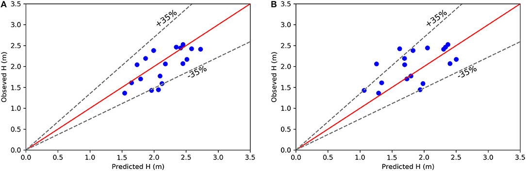
Figure 4. Comparison between predicted and observed flame height values using (A) two-fifths power law and ${\dot{Q}}_{max}$ obtained from ṁ_max [method 1 of Sun et al. (2006)] (B) two-fifths power law and ${\dot{Q}}_{max}$ obtained from ṁ(t_Hmax) [method 2 of Sun et al. (2006)] (n = 18).

Model statistics resulting from the power-law predictions of maximum flame height using method 1 and method 2 are shown in Table 2. For Method 1, the power law correlation had an MAE of 0.1303 (MAPE = 8.61%) with a MBE of 0.1303. For Method 1 MAE is 0.1303, for Method 2 it is 0.1627 (MAPE = 6.83%). Method 2 had a lower MAE using these numbers. A negative MBE was calculated for Method 2, −0.1627. RMSE was lower for Method 2, RMSE = 0.2098 (20.4209 %) than for Method 1, RMSE = 0.3218 (NRMSE = 16.0380%).

TABLE 2

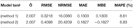
Table 2. Error statistics for maximum flame height power-law correlations using method 1, ${\dot{Q}}_{max}$ obtained from ṁ_max and method 2, ${\dot{Q}}_{max}$ obtained from ṁ(t_Hmax) (n = 18).

Predicted Flame Tilt

Experimental flame tilt angle was obtained from videos by using the computer vision algorithm described in the Methods section. The analysis here represents flame tilts in wind-blown flames. Only configurations with CBH₂ are included. We explored derivation of new semi-empirical correlations applicable for flame tilt angles in chaparral crown fire. Two experiments of wind-blown flames with CBH₂ were analyzed. Power law regression coefficients were obtained from linear regression performed on a log-log plot computed using the Python scipy stats linear regression library. In the first experiment analyzed, hereby called experiment A, the power-law relationship obtained was,

$\begin{array}{ll}\begin{array}{c}tan{\theta }_f=11F{r}^{4.6},R^2=0.85\end{array}& (13)\end{array}$

Observations compared against the power-law given by Equation (13) are presented in Figure 5A. A log-log plot of the data with the corresponding correlation is presented in Figure 5C. A linear regression was performed on the log-log plot in order to obtain the required coefficients.

FIGURE 5

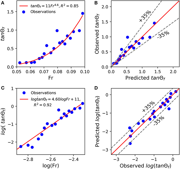
Figure 5. Experiment A, (A) Power-law fit (B) Predicted vs. Observed values based on power law fit (C) log-log fit (D) Predicted vs. observed values based on log-log fit.

The curve shown in Figure 5A shows reasonable agreement between the power-law fit given by Equation (13) and observed data (R² = 0.85). Moreover, observed-vs.-predicted analysis showed that only 10% of flame tilt samples considered fell outside of the 70% accuracy bounds when using this modeling method, see Figure 5B. A sound degree of agreement was consequentially also observed for the log-log analysis (Figures 5C,D).

In the second experiment analyzed, hereby called experiment B, the power-law relationship obtained was,

$\begin{array}{ll}\begin{array}{c}tan{\theta }_f=10F{r}^4,R^2=0.84\end{array}& (14)\end{array}$

Observations compared against the power-law given by (14) are presented in Figure 6A. A log-log plot of the data with the corresponding correlation is presented in Figure 6C. Similarly, to Experiment A, a linear regression on the log-log plot was used to obtain the required coefficients for modeling.

FIGURE 6

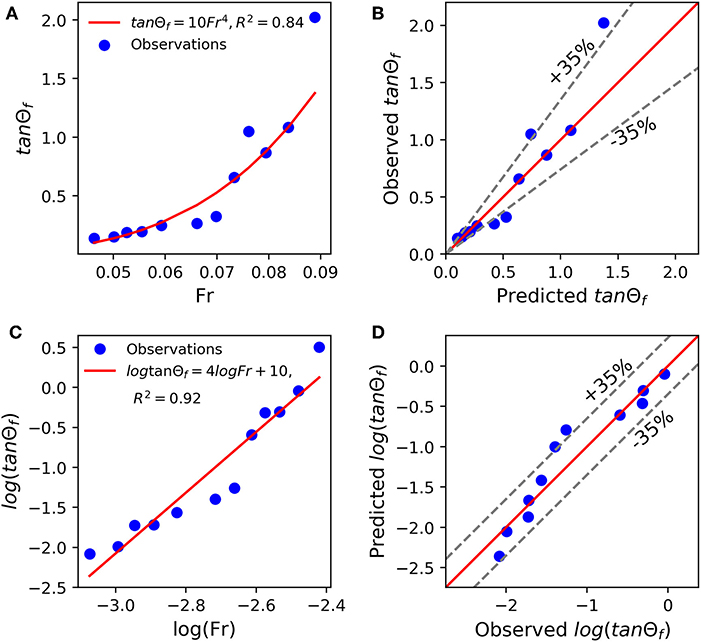
Figure 6. Experiment B (A) Power-law fit (B) Predicted vs. Observed values based on power law fit (C) log-log fit (D) Predicted vs. observed values based on log-log fit.

The power-law correlation represented in Figure 6, shows a reasonable correlation between observed values for Experiment B and Equation (14) (R² = 0.84). Evaluation of observed-vs-predicted values showed that only 30% of flame tilt samples considered fell outside the model 70% accuracy bounds. Reasonable agreement was also observed in the log-log analysis.

Model statistics resulting from the power-law fit on Experiment A and Experiment B are shown in Table 3. For Experiment A, MAE of 0.023 (MAPE = 2.12 %) and an MBE of −0.023 were calculated, hence the model exhibits underprediction of the observed values. For Experiment B, MAE of 0.054 (MAPE = 2.29%) and an MBE of −0.054 were calculated, hence similarly to the model in Experiment B, underpredicting observed values. In addition, RMSE was optimized for the model in Experiment A, where RMSE was 0.14 (NRMSE = 25.23%) as compared to the RMSE for Experiment B which was 0.22 (NRMSE = 36.72).

TABLE 3

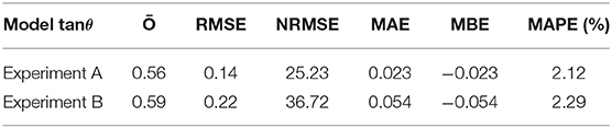
Table 3. Error statistics of flame tilt angle tanθ as a function of Equation 13 for Experiment A and Equation 14 for Experiment B.

Discussion

Flame height results are discussed in terms of model choice and method of heat release rate calculation. In terms of model choice, we evaluated the use of the two-fifths power law given in Equation 2, and the power law derived for dead Fall fuels proposed by Sun et al. (2006) given in Equation 3. Both power laws express flame height in terms of heat release rate. Our results indicate good agreement between flame height values observed experimentally and predicted flame height. Little variation between the two empirical models (Equations 2 and 3) was observed as exemplified by the almost coinciding curves in Figure 3. This suggests the validity of the Fall fuels model, Equation 3, proposed by Sun et al. (2006) for experiments conducted in fire season for chaparral fires modeled as chaparral crown fires.

In terms of heat release calculation method, results showed some variation with respect to flame height obtained from power-law correlations of heat release rate using the time at maximum mass loss rate, Method 1 (${\dot{Q}}_{max,Method1}~\dot{m}(t_{{\dot{m}}_{max}})$), and the time at maximum flame height as a reference, Method 2 (${\dot{Q}}_{max,Method2}~\dot{m}(t_{flameheight,max})$. When using Method 1, only 10% of experiments fell outside the 70% error bounds, whereas this number increased to 17% when using Method 2. Error analysis also reflected slightly larger error measures for Method 2. RMSE was larger for Method 2 than for Method 1. MBE exhibited a negative value only for Method 2, thus potentially hinting at the underprediction of the observed values.

Next, we discuss flame tilt results in terms of two representative experiments analyzed. Overall, we found that for the experiments considered, power-law correlations derived had reasonable accuracy, as exhibited by the calculated R² coefficient of over 0.80 for both experiments. Moreover, over two thirds of samples fell inside the 70% accuracy bounds. Comparison of predicted flame tilt values to values observed experimentally resulted in negative MBE values for Experiment A and Experiment B which could indicate that models obtained for both experiments underrepresented the data. Moving on to MAPE, this measure of error varied by under 1.0 % between the two models. Perhaps the largest variation between statistical error measures of predicted flame tilt was found when assessing RMSE which for Experiment A had a normalized value of 25.23% while for Experiment B this number increased to 36.72%. The difference in RMSE may indicate that model derived using the dataset from Experiment A yielded a closer fit to observed values.

From the analysis presented here, it can be argued that like in other fire spread applications, power-law semi-empirical models may be used to represent fire spreading in the crown fuel layer of chaparral crown fires. The relatively low variation in error between the two models derived here indicate that with further optimization and by considering an expanded dataset, a unified power-law correlation of flame tilt as a function of Froude number could be derived for flames in chaparral crown fires. In assessing results on flame tilt, it was also observed that when estimating flame tilt angle as a function of Froude number in the form given by Equation (6), wind speed did not change and hence, the only varying parameter was flame length or flame height.

Moreover, our results exhibited what could be considered small Froude numbers Fr << 1. The small values points to the dominance of buoyancy forces in governing flame structure. Establishing this feature of fire behavior for the fire system modeled here is significant as it provides information on the modes of heat transfer governing fire spread behavior. This is important as in recent years a great deal of attention has been invested to studying the role of convective and radiative heat transfer in wildland fire behavior. Recent studies examining this aspect of wildfire behavior include those by Finney et al. (2015), Morvan and Frangieh (2018), and Maynard et al. (2016). Results from our work may thus follow others in indicating the role of buoyancy forces driving flame structure and consequently fire behavior. Particular to the work here is a diagnosis on chaparral crown fire fuel beds which illustrates the influence of buoyancy forces on the specific case of crown fire spread and flame behavior in the chaparral. To further understand the role of buoyancy forces in this chaparral crown fire system, future work would benefit from flow visualization such as Schlieren which has been recently used for visualization of convective flow in wildland fire systems (Aminfar et al., 2019).

Summary and Conclusions

The work here aimed to serve as proof of concept on the applicability of certain established models of flame properties to spreading chaparral crown fires. Predictions of flame geometry, particularly flame height and flame tilt angle, were compared to observed values obtained from wind tunnel experiments. Maximum flame height was predicted as a function of maximum heat release rate using power law correlations. Additionally, following Sun et al. (2006), we used two methods to calculate maximum heat release rate. Method 1 where maximum heat release is defined at the time of maximum mass loss rate [${\dot{Q}}_{max,Method1}~\dot{m}(t_{{\dot{m}}_{max}})$] and Method 2 where maximum heat release rate is defined at the time of maximum flame heat ${\dot{Q}}_{max,Method2}~\dot{m}(t_{flameheight,max})$. A good degree of agreement was found between the two-fifths power law correlation of maximum flame height as a function of maximum heat release rate. Similar agreement was found when considering the power-law derived for Fall fuels proposed by Sun et al. (2006).

Error and statistical analysis reflected the positive agreement between predicted and observed values and highlighted some nuances in the predictive potential of the models. Particularly, it was found that Method 1 and Method 2 for maximum heat release estimation showed similar results, but that Method 2 resulted in some degree of underprediction of observed values. However, most other measures of error showed reasonable agreement with observed data. For this reason, it may be concluded that for the conditions tested here, it was shown that the two-fifths power law may in fact be used to predict flame height from maximum heat release rate in chaparral crown fire spread. Fundamental work in studies including that of Thomas (1963) have successfully applied two-fifths power law correlation to spreading natural fires (without wind). More recent studies have successfully applied of these correlations in chamise chaparral burns in pool fire configurations. Despite the fact that the study here was not conducted for pool fire configurations but instead investigated spread fire, the wind conditions tested (1 m/s) are potentially fit for ensuring that for the conditions tested and the fuels considered, the two fifths power law correlation relating flame height to heat release rate does not fail. In future work it would be worth examining whether increasing wind speed would effect any changes in the applicability of this type of correlation. Additionally, here we considered wind-driven and non-wind driven flames as well as two experimental CBH configurations in our assessment of flame height prediction, future work should examine differences in model agreement between the different experimental conditions.

We derived two sample power-law correlations from selected experiments. Error analysis of flame tilt angle predictions obtained from these new power-law correlations showed good agreement between observed and predicted values. The findings in our study lead to the conclusion that in fact, new semi-empirical power-law correlations may be used to express flame height in spreading crown fires as a function of heat release rate. Finally, the results presented here were obtained from selected experiments and as such are representative of the particular conditions tested. We recognize that the models tested and derived here may be limited to the operational conditions assessed and described in the methodologies section of this work. Nonetheless, they represent important steps toward the derivation of new flame property models for chaparral crown fire applications.

Data Availability

The datasets generated for this study are available on request to the corresponding author.

Author's Note

This manuscript was prepared, in part, by a U.S. Government employee on official time, is not subject to copyright and subject to copyright is in the public domain.

Author Contributions

JC-I designed and conducted the experimental study and analyzed data. AA developed codes and computer vision algorithms. DW and MP provided guidance in experimental design and data analysis.

Funding

This work was supported in part by agreement 13JV11272167–062 between USDA Forest Service PSW Research Station and the University of California–Riverside. This research was partially supported by funding from the DOD/DOE/EPA Strategic Environmental Research and Development Program project RC-2640 administered through agreement 16JV11272167026 between the USDA Forest Service PSW Research Station and the University of California, Riverside.

Conflict of Interest Statement

The authors declare that the research was conducted in the absence of any commercial or financial relationships that could be construed as a potential conflict of interest.

Acknowledgments

The authors here would like to thank Gloria Burke and Joey Chong for their assistance during experiments. We would also like to acknowledge and thank Albertina Zuniga, Alejandro Gonzalez, Matthew Choi, Ivan Herrera, and Jake Eagan for their help in experiments and in developing the diagrams presented here.

Footnotes

1. ^The use of trade or firm names in this publication is for reader information and does not imply endorsement by the U.S. Department of Agriculture of any product or service.

References

Albini, F. A. (1981). A model for the wind-blown flame from a line fire. Combust. Flame 43, 155–174. doi: 10.1016/0010-2180(81)90014-6

CrossRef Full Text | Google Scholar

Albini, F. A. (1985). A model for fire spread in wildland fuels by- radiation. Combust. Sci. Technol. 42, 229–258. doi: 10.1080/00102208508960381

CrossRef Full Text | Google Scholar

Alexander, M. E., and Cruz, M. G. (2012). Interdependencies between flame length and fireline intensity in predicting crown fire initiation and crown scorch height. Int. J. Wildl. Fire 21, 95–113. doi: 10.1071/WF11001

CrossRef Full Text | Google Scholar

Aminfar, A., Cobian-iñiguez, J., Ghasemian, M., Espitia, R., Weise, D. R., and Princevac, M. (2019). Using background-oriented schlieren to visualize convection in a propagating wildland fire using background-oriented schlieren to visualize convection in a propagating wildland fire. Combust. Sci. Technol. 0, 1–21. doi: 10.1080/00102202.2019.1635122

CrossRef Full Text | Google Scholar

Barro, S. C., and Conard, S. G. (1991). Fire effects on California chaparral systems: an overview. Environ. Int. 17, 135–149. doi: 10.1016/0160-4120(91)90096-9

CrossRef Full Text | Google Scholar

Bradski, G. (2000). The OpenCV Library. Dr. Dobb's J. Softw. Tools.

Google Scholar

Burger, W., and Burge, M. J. (2008). Principles of Digital Image Processing-Core Algorithms. Berlin: Springer.

Byram, G. M. (1959). “Combustion of forest fuels,” in Forest Fire: Control and Use, ed K. P. Davis (New York, NY: McGraw-Hill, 61–89.

Google Scholar

Cobian-Iñiguez, J., Aminfar, A., Chong, J., Burke, G., Zuniga, A., Weise, D., et al. (2017). Wind tunnel experiments to study chaparral crown fires. J. Vis. Exp. 129, 1–14. doi: 10.3791/56591

CrossRef Full Text | Google Scholar

Cruz, M. G., and Alexander, M. E. (2013). Uncertainty associated with model predictions of surface and crown fire rates of spread. Environ. Model. Softw. 47, 16–28. doi: 10.1016/j.envsoft.2013.04.004

CrossRef Full Text | Google Scholar

Drysdale, D. (2011). An introduction to Fire Dynamics. Second Edition. New York, NY: John Wiley & Sons.

Google Scholar

Fernandes, P. M., Botelho, H. S., Rego, F. C., and Loureiro, C. (2009). Empirical modelling of surface fire behaviour in maritime pine stands. Int. J. Wildl. Fire. 18, 698–710. doi: 10.1071/WF08023

CrossRef Full Text | Google Scholar

Fernandes, P. M., Catchpole, W. R., and Rego, F. C. (2000). Shrubland fire behaviour modelling with microplot data. Can. J. For. Res. 30, 889–899. doi: 10.1139/x00-012

CrossRef Full Text | Google Scholar

Finney, M. A., Cohen, J. D., Forthofer, J. M., McAllister, S. S., Gollner, M. J., Gorham, D. J., et al. (2015). Role of buoyant flame dynamics in wildfire spread. Proc. Natl. Acad. Sci. U.S.A. 112, 9833–9838. doi: 10.1073/pnas.1504498112

PubMed Abstract | CrossRef Full Text | Google Scholar

Gang, C., Ji, J., Zhen, Y., and Ingason, H. (2017). Experimental study of sidewall effect on flame characteristics of heptane pool fires with different aspect ratios and orientations in a channel. Proc. Combust. Inst. 36, 3121–3129. doi: 10.1016/j.proci.2016.06.196

CrossRef Full Text | Google Scholar

Gupta, P., and Gaidhane, V. (2014). “A new approach for flame image edges detection,” in International Conference on Recent Advances and Innovations in Engineering (ICRAIE-2014) (Jaipur: IEEE), 1–6. doi: 10.1109/ICRAIE.2014.6909178

CrossRef Full Text | Google Scholar

Heskestad, G. (1983). Luminous heights of turbulent diffusion flames. Fire Saf. J. 5, 103–108. doi: 10.1016/0379-7112(83)90002-4

CrossRef Full Text | Google Scholar

Heskestad, G. (1984). Engineering relations for fire plumes. Fire Saf. J. 7, 25–32. doi: 10.1016/0379-7112(84)90005-5

CrossRef Full Text | Google Scholar

Maynard, T., Princevac, M., and Weise, D. R. (2016). A study of the flow field surrounding interacting line fires. J. Combust. 2016:12. doi: 10.1155/2016/6927482

CrossRef Full Text | Google Scholar

Morvan, D. (2007). A numerical study of flame geometry and potential for crown fire initiation for a wildfire propagating through shrub fuel. Int. J. Wildl. Fire 16, 511–518. doi: 10.1071/WF06010

CrossRef Full Text | Google Scholar

Morvan, D., and Frangieh, N. (2018). Wildland fire behaviour: wind kW meffect versus Byram's convective number and consequences on the regime of propagation. Int. J. Wildl. Fire 27, 636–641. doi: 10.1071/WF18014

CrossRef Full Text | Google Scholar

Nelson, R. M. (1980). Flame Characteristics for Fires in Southern Fuels. Research Paper SE-RP-205. Asheville, NC: USDA-Forest Service, Southeast Forest Experiment Station, 14. doi: 10.2737/SE-RP-205

CrossRef Full Text

Nelson, R. M., and Adkins, C. W. (1986). Flame characteristics of wind-driven surface fires. Can. J. For. Res. 16, 1293–1300. doi: 10.1139/x86-229

CrossRef Full Text | Google Scholar

Nelson, R. M., Butler, B. W., and Weise, D. R. (2012). Entrainment regimes and flame characteristics of wildland fires. Int. J. Wildl. Fire 21, 127–140. doi: 10.1071/WF10034

CrossRef Full Text | Google Scholar

Padhi, S., Shotorban, B., and Mahalingam, S. (2016). Computational investigation of flame characteristics of a non-propagating shrub fire. Fire Saf. J. 81, 64–73. doi: 10.1016/j.firesaf.2016.01.016

CrossRef Full Text | Google Scholar

Putnam, A. A. (1965). A model study of wind-blown free-burning fires. Symp. Combust. 10, 1039–1046. doi: 10.1016/S0082-0784(65)80245-4

CrossRef Full Text | Google Scholar

Rothermel, R. C., and Philpot, C. W. (1973). Predicting changes in chaparral flammability. J. For. 71, 640–643.

Google Scholar

Steward, F. R. (1970). Prediction of the height of turbulent diffusion buoyant flames. Combust. Sci. Technol. 2, 203–212. doi: 10.1080/00102207008952248

CrossRef Full Text | Google Scholar

Sun, L., Zhou, X., Mahalingam, S., and Weise, D. R. (2006). Comparison of burning characteristics of live and dead chaparral fuels. Combust. Flame 144, 349–359. doi: 10.1016/j.combustflame.2005.08.008

CrossRef Full Text | Google Scholar

Tachajapong, W., Lozano, J., Mahalingam, S., and Weise, D. R. (2014). Experimental modelling of crown fire initiation in open and closed shrubland systems. Int. J. Wildl. Fire. 23, 451–462. doi: 10.1071/WF12118

CrossRef Full Text | Google Scholar

Thomas, P. H. (1963). The size of flames from natural fires. Symp. Combust. 9, 844–859. doi: 10.1016/S0082-0784(63)80091-0

CrossRef Full Text

Thomas, P. H., Webster, C. T., and Raftery, M. M. (1961). Some experiments on buoyant diffusion flames. Combust. Flame 5, 359–367. doi: 10.1016/0010-2180(61)90117-1

CrossRef Full Text | Google Scholar

Van Wagner, C. E. (1977). Conditions for the start and spread of crown fire. Can. J. For. Res. 7, 23–34. doi: 10.1139/x77-004

CrossRef Full Text | Google Scholar

Weise, D. R., and Biging, G. S. (1996). Effects of wind velocity and slope on flame properties. Can. J. For. Res. 26, 1849–1858. doi: 10.1139/x26-210

CrossRef Full Text | Google Scholar

Weise, D. R., Cobian-Iñiguez, J., and Princevac, M. (2018a). “Surface to Crown Transition,” in Encyclopedia of Wildfires and Wildland-Urban Interface (WUI) Fires, ed. S. L. Manzello (Cham: Springer), p. 1–5.

Google Scholar

Weise, D. R., Fletcher, T. H., Cole, W., Mahalingam, S., Zhou, X., Sun, L., et al. (2018b). Fire behavior in chaparral–evaluating flame models with laboratory data. Combust. Flame 191, 500–512. doi: 10.1016/j.combustflame.2018.02.012

CrossRef Full Text | Google Scholar

Williams, F. A. (1985). Combustion Theory, 2nd Edn. Reading, MA: CRC Press.

Google Scholar

Willmott, C. J. (1982). Some comments on the evaluation of model performance. J. Online 63, 1309–1313. doi: 10.1175/1520-0477(1982)063<1309:SCOTEO>2.0.CO;2

CrossRef Full Text | Google Scholar

Zhou, Y., Bu, R., Gong, J., Yan, W., and Fan, C. (2018). Experimental investigation on downward fl ame spread over rigid polyurethane and extruded polystyrene foams. Exp. Therm. Fluid Sci. 92, 346–352. doi: 10.1016/j.expthermflusci.2017.12.009

CrossRef Full Text | Google Scholar

Zukoski, E. E., Kubota, T., and Cetegen, B. (1980). Entrainment in fire Plumes. Fire Safe. J. 3, 107–121. doi: 10.1016/0379-7112(81)90037-0

CrossRef Full Text | Google Scholar

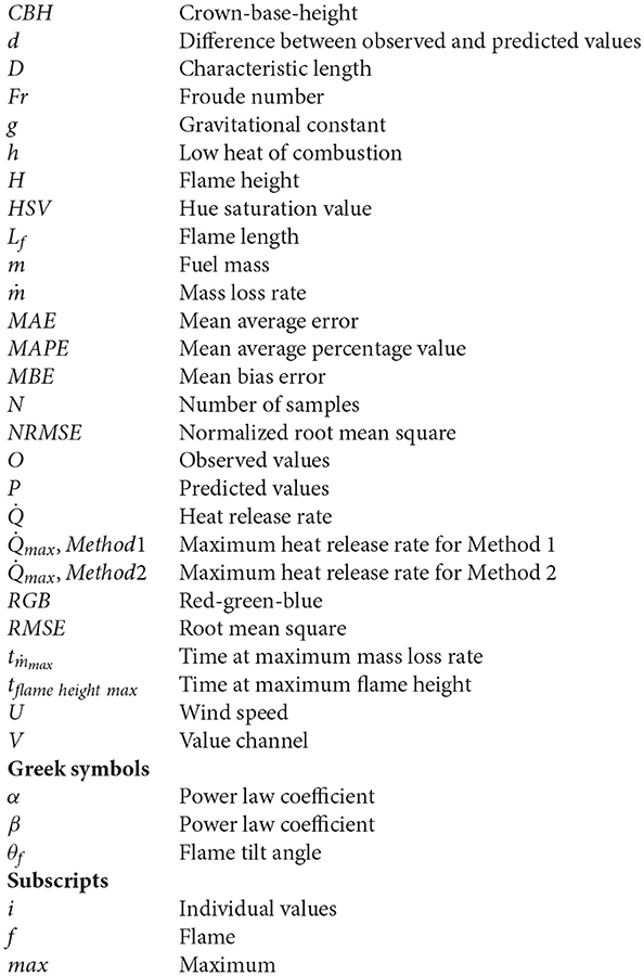
Nomenclature