Modeling Pollutant Emissions of Flameless Combustion With a Joint CFD and Chemical Reactor Network Approach

Introduction

Combustion of fossil fuels and industrial processes were estimated to contribute with around 65% of all anthropogenic greenhouse gases emissions in 2010, while being responsible for ~85% of anthropogenic CO₂ emissions (IPCC, 2014). While there have been efforts to reduce emissions, the global CO₂ emissions have been increasing every year (International Energy Agency, 2018). Most scenarios developed for the future energy supply largely involve the combustion of biofuels, biomass, synthetic fuels, or hydrogen (Ellabban et al., 2014; Scarlat et al., 2015; Nastasi and Basso, 2016). Therefore, progress in combustion technology is necessary for the energy transition and also for the long term solutions that are being considered (Paltsev et al., 2018).

Motivation

Even though the major species of combustion are primarily dictated by the fuel that is being used, the emission of minor pollutant species is dictated by the combustion process. The emission of minor pollutants (CO, NO_x, soot, and unburnt hydrocarbons) have a significant influence on local as well as the global environment. Carbon monoxide (CO) is a harmful substance usually present in flue gases when hydrocarbon or alcohol fuels are employed. Other typical pollutants are nitrogen oxides (NO_x). When air is used as an oxidizer, the formation of NO_x tends to occur during combustion as the N₂ contained in air dissociates in the combustion reactions (Glarborg et al., 2018). The NO_x emission from aircraft cruising in the upper layers of the troposphere or in the lower layers of the stratosphere is responsible for the formation of ozone (Grewe et al., 2012). At lower altitudes, the NO_x emission is directly linked to respiratory diseases (World Health Organization, 2013), and is responsible for the acidification of water and rain that harms vegetation and wildlife (Camargo and Alonso, 2006). Therefore, there are tight regulations for the emission of CO and NO_x and future restrictions on these emissions are being tightened, thereby posing challenges to designers of combustion systems.

One of the promising combustion technologies to lower pollutant emissions is the Flameless Combustion (FC) regime. Despite the fact that the FC regime does not have a clear and universally accepted definition, or that its physics are not yet fully understood (Perpignan et al., 2018a), it is clear that the regime has potential to substantially decrease emissions. Usually characterized by distributed reaction zones with lower temperature and species gradients, FC was shown to yield low NO_x emissions while maintaining low CO (Kruse et al., 2015).

The modeling of FC is still challenging. Particularly, modeling tools able to predict pollutant emissions are required in order to assess, design and improve devices reliant on the regime. The use of Computational Fluid Dynamics (CFD) for modeling combustion largely relies on the use of simplified chemistry, as detailed chemical reaction mechanisms composed of hundreds of species and reactions cannot be accommodated at reasonable computational costs. Apart from the sheer number of reaction, solving detailed chemistry also adds the complexity of dealing with the wide range time-scales of the various chemical reactions, which causes the systems of equations to be stiff. Usually, the focus and strength of CFD has been on predicting reaction zone structures, temperatures and velocities, and not pollutant emissions.

CRNs for Emission Prediction

The lack of detailed chemical schemes has been pointed out as the main cause of discrepancy often seen between CFD and experimental results in emissions (Lyra and Cant, 2013). Because of that, the use of Chemical Reactor Networks (CRNs) to predict pollutant emissions has gained attention. A CRN is a set of ideal chemical reactors, in which detailed chemical reaction mechanisms can be applied at relatively low computational costs. On the other hand, most approaches developed for CRNs neglect turbulence-chemistry interaction and complex flow structures.

The design of CRNs manually has provided valuable results. The designs are usually based on experimental results or CFD simulations. The work of Lebedev et al. (2009) presented a CRN composed of six reactors to model a gas turbine combustor. The authors defined the CRN based on the mixture fraction field predicted via CFD. Likewise, utilizing velocity, temperature and species fields coming from CFD simulations, Park et al. (2013) developed a CRN to model a lean-premixed gas turbine combustor and obtained good matches with respect to experimental data.

More recently, Prakash et al. (2018) studied the effect of exhaust gas recirculation (EGR) on the emissions of a lean premixed gas turbine combustor using a manually designed CRN. The adoption of EGR might cause the required conditions for FC to occur, as O₂ concentrations drop and initial temperatures rise. Studying FC, the work of Perpignan et al. (2018b) showed the results of a CRN manually built based on CFD made with the Flamelet Generated Manifolds (FGM) approach, which is also employed in the present work. The authors achieved better agreement with CO and NO_x experimental data using the CRN than with the reacting CFD. The focus was on a gas turbine combustor designed to operate under the FC regime. The detailed chemistry enabled the analysis of the NO_x formation pathways, showing that the thermal pathway is not as important as the prompt, NNH and N₂O pathways. This showcases the capability of in-depth chemistry analysis when utilizing CRNs.

The application of CRNs to predict emissions from FC systems has, in principle, advantages when compared to conventional combustion systems (Perpignan et al., 2018a). The highly distributed reaction zones, as well as lower gradients of species and temperatures, are better represented by ideal reactors (Cavaliere and de Joannon, 2004). However, this observation is valid for the largest scales, as there is evidence FC might be composed highly interactive flamelets at the smaller scales (Minamoto et al., 2013, 2014; Minamoto and Swaminathan, 2014).

The manual generation of CRNs is, nonetheless, particularly reliant on the experience of the designer and suffers from the lack of repeatability as a significant amount of trial and error approach is involved. Additionally, creating networks manually impedes the reproducibility of results and hampers systematic studies. As an attempt to avoid these issues, strategies to generate CRNs automatically based on CFD solutions have been developed.

Early applications of automatic CRN generation were employed in simulations for analyzing furnaces (Benedetto et al., 2000; Faravelli et al., 2001; Falcitelli et al., 2002). Promising results were achieved as 3D CFD simulations were post-processed. The works utilized temperature and stoichiometry to define the ideal reactors, which could be PSRs or PFRs, based on the angle of the velocity vector. The underlying assumption was that the simplified chemistry models employed in the CFD were enough to predict temperature, velocity and major species. Moreover, these works provided insights into important variables to be taken into account when clustering CFD cells: temperature, a variable capturing the flow direction, and at least one measure of composition.

The same computational tool (with the same clustering criteria) was employed by Frassoldati et al. (2005) in the case of the swirling flame of the TECFLAM burner test case. The authors showed the effect of varying the number of reactors on the result of NO_x emissions. For that specific case, having 300 reactors proved to be enough to guarantee no significant variation with a further increase in the number of reactors. Good agreement with the outlet value of NO_x was shown, as only one operating condition was simulated.

Fichet et al. (2010) presented another strategy to use a CFD solution as an input to build a CRN. The authors utilized a gas turbine combustor to showcase the capabilities of the approach. They opted for discarding the temperatures calculated with CFD and recalculated the temperatures based on the heat release of the chemical reactions predicted by the CRN. There was no systematic study on the advantages and disadvantages of this approach. The authors reported good agreement between measured and simulated NO_x emissions. However, only one operating condition was available.

Similarly, Monaghan et al. (2012) utilized the Sandia Flame D as a test case and post-processed a CFD solution to build CRNs. The authors reported improved results for minor species (OH and NO) with respect to the initial CFD solution. The strategy to cluster CFD computational cells into reactors involved using mixture fraction, temperature and the axial coordinate.

In yet another example, Cuoci et al. (2013) utilized a few test cases to explore their computational tool, including the one utilized in the present work, presented in section The Test Case. The authors analyzed one of the operating conditions to which they reported improved NO_x predictions, while CO was overpredicted to some extent. According to the authors, the source of deviation in NO was the incorrect temperatures predicted by the CFD simulations.

Despite the valuable developments, the full potential and limitations of using both CFD and CRN are not fully known. For example, the effect of different clustering criteria on the final solution is not clear, and that is one of the objectives of the present work. Additionally, there are other unknowns in the approach, as the effect of neglecting turbulence chemistry-interaction or taking it into account (via a PaSR—Partially Stirred Reactor approach, for example), or the pros and cons of solving the energy equation in the CRN step.

For these reasons, Automatic Generation of Networks for Emission Simulation (AGNES) (Sampat, 2018) was developed at the Delft University of Technology. The computational tool uses Cantera (Goodwin et al., 2018), an open-source software dedicated to chemical kinetics as a framework. Yousefian et al. (2017) reviewed the available hybrid computational tools based on CRNs for emissions predictions. In their evaluation of the different available solvers for CRNs, the authors highlighted two of the characteristics of Cantera that made it attractive for the development of AGNES: the capability of solving the energy equation and the fact that it is a free and open source solver, as further discussed in section Chemical Reactor Networks. Being able to modify and control the code was essential for the development of AGNES.

In the present paper, AGNES is utilized to simulate a test case related to the FC regime, in order to showcase its capabilities, limitations, and improvement opportunities. Additionally, the analysis of the results aims to clarify the reasons for the emission behavior in the chosen test case. The unique contribution of the present research is the assessment of different clustering criteria on the outlet emissions of an FC system that has a complex NO_x behavior with varying equivalence ratio, as shown in section The Test Case.

The Test Case

In order to evaluate the performance of AGNES, a test case was chosen based on the available information and the relevance to FC. Data availability on emission characteristics of the combustor for various operating conditions was a stringent requirement in making the selection. The test case described by Veríssimo et al. (2011) was chosen as a test case. The combustor was developed to study FC in a non-premixed combustion mode. The combustor consists of a cylindrical combustion chamber with a central air jet surrounded by 16 fuel jets in the burner head. This configuration is a variation of the most common jet-induced recirculation geometry in which a central fuel jet is surrounded by air jets (Hosseini and Wahid, 2013). The inlet air was preheated to 673.15 K, while the fuel (pure methane) was at room temperature.

The equivalence ratio was varied by maintaining the fuel mass flow (heat input of 10 kW) and altering the air mass flow. Data on OH^* chemiluminescence, flue-gas temperatures and, more importantly, emissions of CO and NO_x were acquired for all operating conditions. The equivalence ratio was varied from ϕ = 0.455–0.909 and the behavior of CO and NO_x emissions was found to be non-monotonic. The authors reported a peak in NO_x around ϕ = 0.53, while CO was practically undetectable for the runs at ~ϕ = 0.53 and 0.59 (see Figure 1).

FIGURE 1

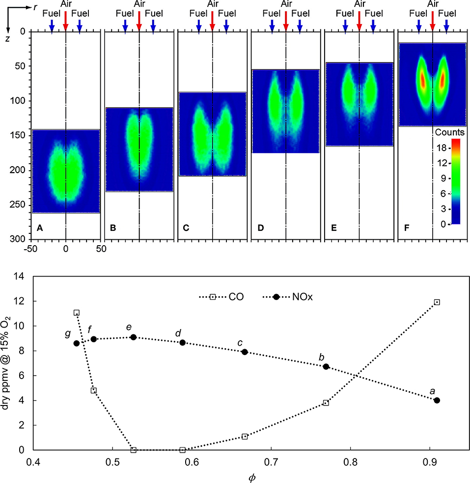
Figure 1. Mean OH* images for diverse global equivalence ratio values. From left to right, ϕ ≅ 0.91, 0.77, 0.67, 0.59, 0.53, 0.48 (Above). Emissions of NO_x and CO in dry volumetric ppm adapted from Veríssimo et al. (2011) (Below).

This behavior was explained by the authors based on a combined effect of the global equivalence ratio and the mixing characteristics of the combustor. Starting from condition a in Figure 1 and going toward leaner conditions, more air flow was added. The higher central air jet momentum was responsible, according to the authors, for quicker and stronger entrainment of the fuel, which had weaker jets. The stronger mixing of fresh reactants caused more intense reaction zones (as shown in Figure 1), while not allowing as much mixing of combustion products prior to the reactions. The result was then higher NO_x and lower CO. This trend was dominant up to conditions e or f , in which the usual pattern of having lower NO_x and higher CO as going leaner becomes dominant over the mixing characteristics.

In a more recent study, Zhou et al. (2017) performed OH and CH₂O PLIF on the same setup, and referred to operating conditions a, c, and e as flameless, transition and conventional modes, respectively. They support that conditions e and f behave like conventional diffusion flames, as mixing with combustion products is apparently minimal and combustion is dictated by the mixing between fuel and air. As mixing with combustion products is allowed by the weaker entrainment of fuel by the air jet, the combustion regime transitions to FC. A summary of the operating conditions with ϕ, air mass flow rate and outlet O₂ concentration is shown in Table 1.

TABLE 1

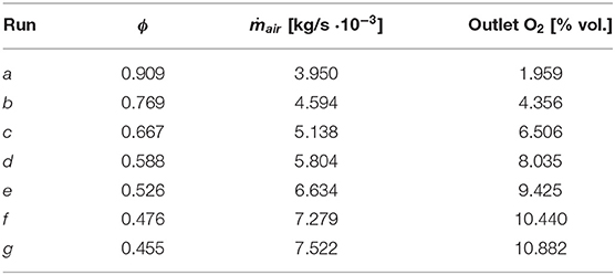
Table 1. Operating conditions investigated by Veríssimo et al. (2011).

For conditions b and d, Veríssimo et al. (2011) provided point-measurements at various radial stations. Temperatures, major species (CO₂ and O₂) and pollutants (CO, UHC, and NO_x) were measured at 10 radial positions at each of the 10 stations.

The test case was simulated before, by Cuoci et al. (2013) and Lamouroux et al. (2014), for example. However, the focus of these previous works was on local values and a single operating condition for the former, and on the effect of including heat losses on local values for the latter. The focus of the present work is instead on the outlet emissions of CO and NO_x across different operating conditions.

Computational Modeling

In an attempt to overcome the challenges in predicting emissions at affordable computational costs, a three-step approach is adopted in the current research: (1) solution of the flow-field with CFD using simplified chemistry and a turbulence-chemistry interaction model, (2) clustering of computational cells into ideal reactors based on criteria imposed to the CFD solution, and (3) solution of the generated CRN with detailed chemical reaction mechanisms. In the following subsections, the details of these steps are presented.

The specific objectives of the performed modeling are:

i. Evaluating the performance of the chosen CFD modeling

ii. Evaluating the performance of the developed computational tool

iii. Comparing the results obtained with CFD and CRNs

iv. Obtaining minor species concentration more accurately than those obtained with the CFD simulations used as input to the CRN simulations

v. Analyzing the NO_x formation pathways for different operating conditions of the combustor

Computational Fluid Dynamics

The simulations were performed in order to assess the performance of CFD in predicting pollutant emissions and, more importantly, to generate the inputs for the subsequent modeling steps. The RANS (Reynolds Averaged Navier-Stokes) approach was adopted along two different turbulence-chemistry interaction models: EDM (Eddy Dissipation Model) (Magnussen and Hjertager, 1976) and FGM (van Oijen and De Goey, 2000). All simulations were performed in ANSYS Fluent^®. The EDM was chosen to perform a comparison with FGM. The assumption behind the model is that reactions are chemically fast and are controlled by turbulent mixing. Therefore, it was not expected that the EDM would perform accurately, at least not for all the operating conditions of the chosen test case. The EDM is possibly the simplest turbulence-chemistry interaction model and the objective of utilizing it was to assess how the quality of the CFD simulation utilized as input affects the results obtained solving the resulting CRNs.

A two-step reaction mechanism was adopted for CH₄ combustion, as shown by Equations (1) and (2). The EDM determines the reaction rates based on large turbulence time scales (k/ε), as shown in Equation (3) (Magnussen and Hjertager, 1976).

$\begin{array}{ll}{\text{CH}}_4+\text{1}.\text{5 }{\text{O}}_2\leftrightarrow \text{CO}+\text{2 }{\text{H}}_2\text{O}& (1)\end{array}$

$\begin{array}{ll}\text{CO + 0}.\text{5 }{\text{O}}_2\leftrightarrow {\text{CO}}_2& (2)\end{array}$

$\begin{array}{l}{R}_{i,r}=\left(4C_{i,r}{M}_i\rho \frac{\epsilon }{k}\right)\min [{\min }_{reac.}\left(\frac{Y_{reac.}}{C_{reac.,r}{M}_{reac}}\right),\\ 0.5\frac{{\displaystyle {\sum }_{prod}{Y}_{prod.}}}{{\displaystyle {\sum }_{prod}^N{C}_{prod.,r}{M}_{prod.}}}]& (3)\end{array}$

The choice for FGM was based on its relatively low computational cost with respect to other models (Eddy Dissipation Concept, Conditional Source-term Estimation or transported-PDF, for example), and on its performance for various combustion systems (Verhoeven et al., 2012; van Oijen, 2018). This approach has shown to be promising for the modeling of FC, provided the progress and control variables are adequately chosen (Perpignan et al., 2018a). The approach allows the use of detailed chemistry in the pre-calculation generation of flamelets. Non-premixed flamelets were chosen due to the nature of the analyzed burner, and were solved using the GRI 3.0 chemical reaction mechanism (Smith et al.). Tests were performed utilizing the GRI 2.11 (Bowman et al.) and the POLIMI C1-C3 (Ranzi et al., 2012) mechanisms, but no significant differences were observed.

The underlying assumption of the FGM model, or any flamelet-based approach for turbulent combustion, is that a turbulent flame can be represented as an ensemble of laminar flames. The flamelets were calculated in the mixture fraction space according to Equation (4), for species, and Equation (5), for temperature, according to the formulation of van Oijen and De Goey (2000). The pre-calculated flamelet quantities were then tabulated based on mixture fraction, a predefined progress variable and enthalpy, which are the variables that require transport equations. A presumed β shape PDF was employed to account for the turbulence-chemistry interaction, which was a function of the mean and variance of the mixture fraction.

$\begin{array}{ll}\rho \frac{\partial Y_i}{\partial t}=\frac{\rho \chi }{2}\frac{{\partial }^2{Y}_i}{\partial f^2}+S_i& (4)\end{array}$

$\begin{array}{ll}\rho \frac{\partial T}{\partial t}=\frac{\rho \chi }{2}\frac{{\partial }^{2}T}{\partial f^2}-\frac{1}{c_p}{\displaystyle \sum _i}{S}_i{H}_i+\frac{\rho \chi }{2c_p}\left[\frac{\partial c_p}{\partial f}+{\displaystyle \sum _i}{c}_{p,i}\frac{\partial Y_i}{\partial f}\right]\frac{\partial T}{\partial f}& (5)\end{array}$

The adopted progress variable as assumed to be dependent on the mass fraction of CO and CO₂. Tests performed including H₂O and H₂ in the definition of the progress variable, species adopted by previous works, did not provide better results for this case. In order to calculate NO_x species from the CFD simulations to perform a comparison with the results of AGNES, additional transport equations for NO, HCN, N₂O, and NH₃ were included. Reactions representing the thermal, prompt, and N₂O pathways were considered. Reaction rates of NO_x species accounted for the temperature fluctuations by means of a β-PDF.

The closure for the RANS equations was achieved using the k-ε turbulence model. Since the burner has round air and fuel jets, the C_ε1 constant was adjusted to 1.6 to correct for the well-known round jet anomaly (Pope, 1978; Shih et al., 1995). Tests using a Reynolds Stress model did not provide superior results.

The modeling of heat loss is extremely important for the prediction of the temperature and the resulting emissions. The modeling of radiation was performed with the Discrete Ordinates model along with the weighted-sum-of-gray-gases approach to determine the required fluid properties. Heat conduction through the walls was imposed via wall temperature profiles. The profiles were determined partially based on the reported temperature values 5 mm from the walls for conditions b and d, as well as the outlet temperature. The profiles were first estimated by extrapolating the available data at the radial locations to the wall location. Subsequently, the resulting profile at the wall was multiplied by a factor to meet the outlet temperatures obtained in the experiments, thereby resulting in the same overall heat loss. For conditions in which local measurements were not available, linear interpolations and extrapolations of the profiles were performed, based on the equivalence ratio.

The computational mesh used was fully hexahedral and a 45° sector was simulated, which included two fuel ports, as shown in Figure 2. The angle was adopted to guarantee a good mesh quality in terms of skewness. The mesh refinement was defined based on monitoring the outlet values of chemical species, as well as mid-plane averaged quantities, to guarantee no significant changes were attained with further refinement. The initial mesh size was ~1 million elements and other four mesh sizes were tested until the difference in outlet species and averaged quantities was negligible. The final mesh was composed of ~2.5 million elements.

FIGURE 2

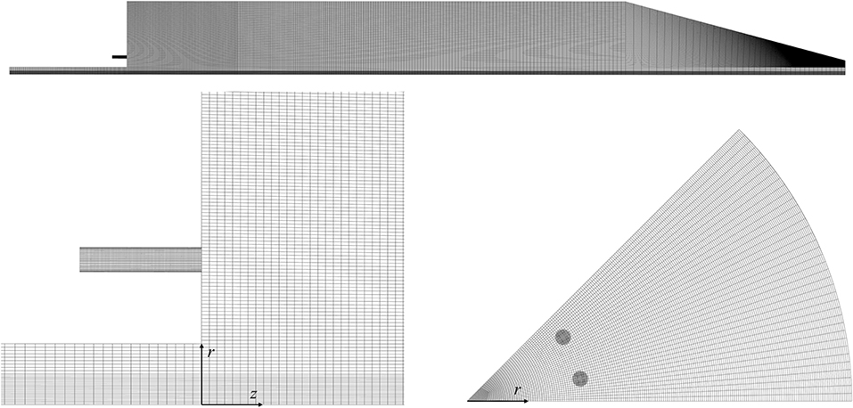
Figure 2. Hexahedral mesh employed for CFD simulations.

Periodicity was imposed on the lateral boundaries. The first set of simulations was performed with mass flow inlets of air and fuel with uniform profiles. As the effect of having a developed flow velocity profile imposed as the boundary was shown to influence the results, this was adopted for the simulations herein reported. The developed flow velocity profile was assumed to follow Equation (6), a power-law velocity profile. The turbulence intensity was assumed to be 5% of the mean velocity. Tests with increased intensity did not significantly affect the results. Turbulence length scale at the boundaries was estimated based on the pipe diameters for both air and fuel, as it was imposed to be 7% of these dimensions. The outlet boundary condition was imposed to have zero static gauge pressure.

$\begin{array}{ll}\frac{u}{u_{max}}={\left(1-\frac{r}{(D/2)}\right)}^{\frac{1}{7}}& (6)\end{array}$

Chemical Reactor Networks

In order to simulate combustion with detailed chemistry at affordable computational costs, AGNES was employed. Having the results from the CFD simulations, the tool first clusters computational cells into reactors based on user-defined criteria. Clustering is executed with a Breadth First Search (BFS) algorithm used to traverse the computational domain. Such a domain traversal algorithm was chosen to ensure that the clustered cells are indeed connected to each other in the mesh, forming a continuous domain, and preventing the clustering of discontinuous pockets of cells satisfying the criteria. The clustering process proceeds until the total number of reactors (clusters) reaches the set-point imposed by the user, or until the specified maximum tolerance is attained. The quantity range value α is defined as shown in Equation (7), and it is dependent on a certain tolerance δ. The new local value, calculated by averaging the clustered cells, is allowed to deviate from the original local value as expressed by Equation (8). Several variables can be used simultaneously as criteria and every criterion must be satisfied for a cell to be included in a cluster.

$\begin{array}{ll}\alpha =\delta (c_{max}-c_{min})& (7)\end{array}$

$\begin{array}{ll}\alpha \ge |c_{cluster}-c_{cell}|& (8)\end{array}$

The resulting reactors have their properties assigned based on the properties of the CFD cells that compose the reactors. When maintaining temperatures as obtained from the CFD solution, which is the case for the present paper, averaged static temperatures are assigned, although total values are used during clustering to guarantee total enthalpy conservation.

The mass flow exchanged between reactors is calculated based on the mass flow between cells in the CFD solution. There is an inherent mass imbalance due to the precision of the CFD solution which needs to be corrected to ensure consistent mass conservation. This is done by accounting for the mass flow between any two reactors as a fraction of the total outflow from the source reactor and assembling a system of equations. The boundary conditions of total inflow and outflow are accounted for in the system. The system of equations (mass, species, and energy conservation) is solved for, giving a vector of total outflow from each reactor and the “corrected” mass flow between reactors is recalculated using this vector and the matrix of outflow fractions. The mass exchange between reactors is also stored and maintained when solving the CRN simulation.

The system of ODEs is characterized by non-linearity and stiffness. The stiffness of the system is attributed to the wide range of time scales encountered for the reactions involved. Some reactions, such as those responsible for heat release, are much faster than those responsible for the formation of minor species such as that of NO_x. This makes it difficult to integrate as the fast reactions require a small time step to be captured whereas the slow reactions need to be integrated over a larger time scale. Therefore, two levels of solvers are implemented, a local and a global. The local solver treats each reactor individually, whereas the global solver treats all the reactors simultaneously as a system. Cantera is used in the following ways:

i. As a chemistry book keeping tool, in which Cantera ensures a consistent physical and chemical state of the reactors in the form of their temperature, density, and species mass fraction and storing the chemical reaction mechanism with all its thermodynamic properties.

ii. It can also be used to solve a reactor network, in which Cantera calls SUNDIALS to perform ODE integration of a stiff system of equations, while treating it as a dense matrix.

At the local solver level, both features are used, whereas at the global solver level Cantera is used only as a chemistry book keeping tool, as shown in Figure 3. This is due to Cantera's solver limitations of being unable to simultaneously handle large number of reactors, hence the governing equations are written explicitly and solved using SciPy, a Python-based ecosystem for mathematics, science, and engineering, to solve a sparse matrix equation for the entire network of reactors.

FIGURE 3

Figure 3. Flowchart of AGNES.

As previously mentioned, both a local and a global solver are employed. Locally, the solver available in Cantera is used to advance each reactor individually, changing its state and that of its connected reservoirs. This solver employs a different time-step to each reactor, based on its residence time. The global solver employs Cantera only to maintain the consistency of the chemical states, while all reactors are solved simultaneously with the sparse solver.

All reactors were considered to be PSRs. No turbulence fluctuation was taken into account in the CRNs. They were neglected because approaches with and without the inclusion of fluctuations are still being successfully employed (Yousefian et al., 2017) and a logical first step in the development of AGNES was to start without them. Moreover, this first application of AGNES is aimed at investigating the effect of clustering criteria on the solution. The inclusion of fluctuations may be important in some cases, as shown by Cuoci et al. (2013). For this reason AGNES will be modified to be capable of including fluctuations in the future.

The results herein presented were obtained by imposing a 3% tolerance. This resulted in different numbers of reactors for each test condition and imposed clustering criteria. Simulations were performed with both GRI 3.0 and GRI 2.11 mechanisms, to investigate the effect on NO_x formation, as it has been shown that there are relevant differences in the NO_x formation pathways under FC conditions (Perpignan et al., 2018b).

Several tests with various clustering criteria were performed in order to evaluate their efficacy to the present test case (Sampat, 2018). Apart from the obvious choice of temperature as a criterion, it was observed that the inclusion of velocity direction as a criterion was fundamental to capture the recirculation within the combustor, a key for capturing the chemistry within FC. Additionally, a variable acting as a tracer of the fuel, as well as a variable indicating the progress of reactions were required. In the present work, these are the Y_CH4 and Y_H2O, respectively. Two sets of criteria are explored, one with the aforementioned variables, and one with the inclusion of Y_O2.

Results

In this section, the results obtained from CFD simulations are presented and discussed. The extent to which the CFD modeling was able to replicate the experimental data is shown, in terms of temperatures, major species and pollutant emissions. Subsequently, the results obtained with AGNES are thoroughly analyzed.

CFD Results

As expected, the FGM simulations showed better results when compared to the EDM, as shown in Figure 4. The temperature rise occurs earlier in FGM, better representing the experimental data points. It is worth noting the discrepancy between experimental and simulation values in the data point (z/D = 0.11). This difference might be attributed to the heating of the burner head and its piping, which might have caused the pre-heating of air to a temperature higher than that reported by the authors. Another hypothesis would be the effect of radiation on the thermocouple, although the authors assessed this effect. The error in temperature measurements was estimated by Veríssimo et al. (2011) to be around 5% (as is shown by the error bars in Figure 4).

FIGURE 4

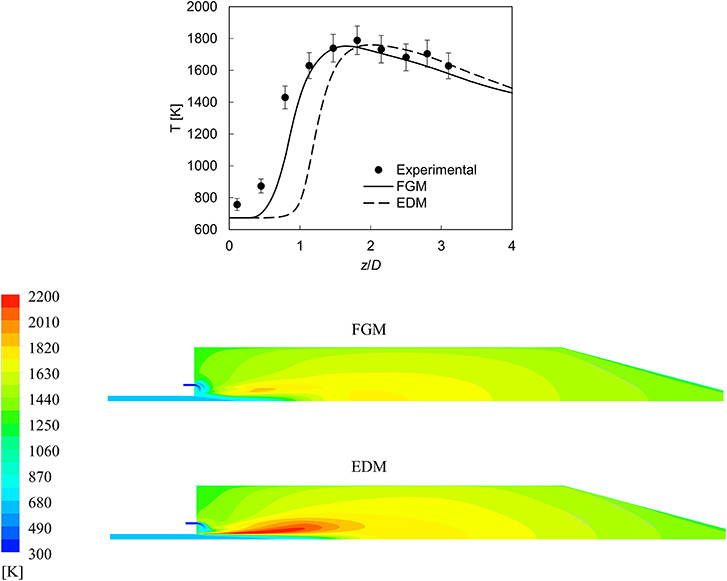
Figure 4. Experimental and CFD temperature results along the centerline of the combustor (Above) and temperature contour plots (Below) for condition b (ϕ ≅ 0.77) using FGM and EDM.

Although the centerline values of temperature shown in Figure 4 depict that FGM was superior, the extent of that is not well-represented. The peak temperatures attained in the combustor are not located at the centerline, but at the region where fuel and air mix. In this region, EDM peak temperatures are much higher than those predicted by FGM, as seen in the contours of Figure 4. Additionally, looking only at the centerline values shown in Figure 4 it may seem that reactions with FGM occur faster than with EDM, but that is not the case.

A major difficulty in simulating the case at hand is the uncertainties related to heat losses. Radiative heat losses play a role in the combustor, as well as conduction through the walls. The total heat loss can be derived by the reported values of outlet temperatures, although the exact location where the temperatures were measured is not fully clear. Therefore, a wall temperature profile was imposed based on the results available at 5 mm from the wall (r/D = 0.45), attempting to maintain them as close as possible. Temperature at this position is, however, not only dependent on the wall temperatures, but also on the reaction rates, recirculation, and radiation. The extent to which the simulations are able to reproduce these values is shown in Figure 5.

FIGURE 5

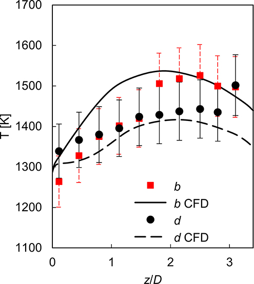
Figure 5. Experimental and CFD temperature results along the axial line where r = 45 mm for conditions b (ϕ ≅ 0.77) and d (ϕ ≅ 0.59).

The centerline values of O₂ and CO₂ shown in Figure 6 indicate that predictions for condition d were more accurate than for the condition b. The reasons for this may be related to the fact that condition d is, according to Veríssimo et al. (2011) and Zhou et al. (2017), closer to a conventional diffusion flame, while condition b would be more representative of FC, making it more difficult to model, as a control variable representing vitiated recirculated gases may be required for the representation of FC with FGM (Huang et al., 2017). However, the values of CO₂ and O₂ close to the outlet should not be dependent on the combustion regime or the type of modeling. As also shown in Figure 7, simulations for condition b have higher CO₂ and lower O₂ values at the outlet. The discrepancy between simulations and experimental values on the O₂ values close to the outlet for condition b has been shown before in the results of Cuoci et al. (2013). The experimental uncertainty of 10% in the composition data does not justify the difference alone. Therefore, the uncertainty of the reported mass flows is probably causing the discrepancies.

FIGURE 6

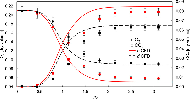
Figure 6. Experimental and CFD results along the centerline of the combustor for O₂ and CO₂ concentrations for conditions b (ϕ ≅ 0.77) and d (ϕ ≅ 0.59).

FIGURE 7

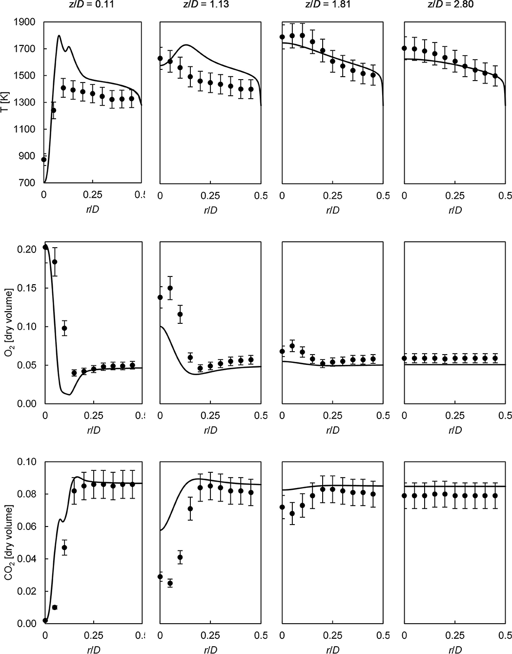
Figure 7. Comparisons of experimental and CFD (FGM) parameters: temperature, O₂ concentration, and CO₂ concentration results along radial lines for condition b (ϕ ≅ 0.77).

The overall agreement between experimental data and the FGM simulations is good (Figures 7, 8). The largest deviations for temperatures occur closer to the burner head (z/D = 0.11), especially for condition b. Further downstream in the combustion chamber, the agreement is better. Simulations presented the overall characteristic of retaining lower temperatures near the centerline for longer axial distances, while combustion was more progressed (i.e., lower O₂ and higher CO₂ concentrations). This can be explained by a possible imperfect prediction of the mixing between burnt gases and reactants, as well as the effect that burnt gases have on the incoming reactants. Moreover, the aforementioned apparent inconsistency in temperature modeling (or measurements) close to the burner head, as well as the uncertainty related to mass flows might also have contributed.

FIGURE 8

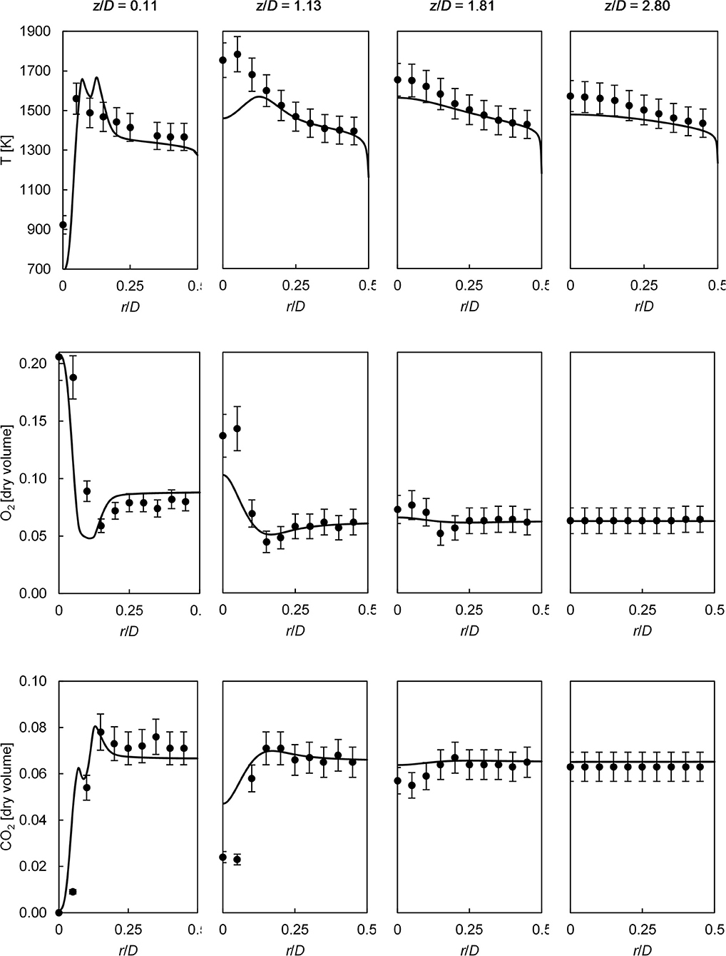
Figure 8. Comparisons of experimental and CFD (FGM) parameters: temperature, O₂ concentration, and CO₂ concentration results along radial lines for condition d (ϕ ≅ 0.59).

The radial profiles (Figures 7, 8) show that the effects of the central jet spreading rate seem to be overpredicted in the simulations. This can be noticed by the fact that the gradients of the profiles tend to be lower than those obtained in the experiments for intermediate axial positions (z/D = 1.13 and 1.81). This was also the case in the reported previous computational works on the same test case (Cuoci et al., 2013; Lamouroux et al., 2014). However, the discrepancies could also be a result of poor prediction of reaction rates or heat transfer, instead of an artifact of the jet spreading prediction.

The predictions of pollutant emissions from the CFD modeling is poor, both in terms of the absolute values as well as in the trends (Figure 9). The emission of CO is highly overpredicted, in some conditions up to two orders of magnitude. The NO prediction is, on the other hand, underpredicted. The trend of NO is also not captured, as values increase monotonically with increasing ϕ. These results were to a certain extent expected, as the accurate prediction of CO with FGM is challenging (Ramaekers et al., 2010) and the NO_x species modeling was not based on a detailed chemical reaction mechanism.

FIGURE 9

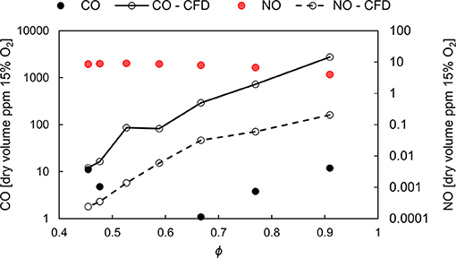
Figure 9. Outlet CO and NO results from CFD performed with FGM compared with experimental values.

Finally, the CFD results based on FGM performed reasonably well in order to be used as an input to the CRN simulations. Most of the variables have a good level of agreement (apart from pollutants). Better results could be expected by utilizing an FGM approach that is more suitable for modeling FC, such as the diluted-FGM, developed by Huang et al. (2017). Perhaps the mixing in the combustor has unsteady characteristics which can be captured adequately only by LES. However, previous attempts of simulating the test case with LES along with tabulated chemistry did not provide improved results (Lamouroux et al., 2014).

AGNES Results

The results obtained from the CRN simulations performed with AGNES are discussed herein with respect to the combustion model obtained from the CFD input (FGM or EDM), to the clustering criteria, and chemical reaction mechanism.

The CO predictions are improved significantly with respect to the CFD simulations performed with FGM, regardless of the clustering criteria (Figure 10). The same is valid for simulations based on the EDM, in which the main difference with respect to FGM is in the predictions of CO for conditions closer to stoichiometry. All results predict the trend of CO and have fairly similar values. Additionally, no significant difference between GRI 3.0 and GRI 2.11 can be noticed.

FIGURE 10

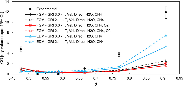
Figure 10. Outlet CO results from AGNES compared with experimental results. Different input simulations for AGNES (FGM or EDM) and post-processing options (GRI 3.0 or GRI 2.11, as well as clustering criteria).

The calculated NO_x values based on the EDM simulations are overpredicted, as expected (Figure 11). The high peak temperatures attained with the modeling are responsible for the results being up to one order of magnitude higher. The results obtained from FGM are more complex to analyze (Figure 12). When temperature, velocity direction, Y_CH4 and Y_H2O are employed as clustering criteria, the NO_x trend obtained with GRI 2.11 reaction mechanism is monotonic and its slope is the opposite of the experimental data: condition a had the highest NO_x value. For GRI 3.0, overall values are higher than those of GRI 2.11 (a behavior previously reported by Perpignan et al., 2018b), but condition a has a lower value than condition b, making the overall trend non-monotonic. The values, however, are not in good agreement with experiments for both chemical reaction mechanism.

FIGURE 11

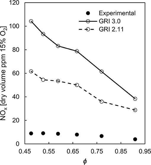
Figure 11. Outlet NO_x results from AGNES having CFD simulations performed with EDM as input compared with experimental results.

FIGURE 12

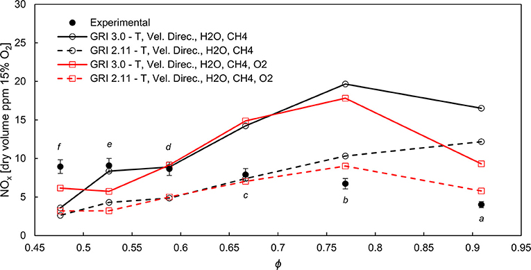
Figure 12. Outlet NO_x results from AGNES having CFD simulations performed with FGM as input compared with experimental results. Two different clustering criteria sets.

The inclusion of Y_O2 as a clustering criterion is fundamental to attain a trend closer to experimental data with respect to the non-monotonic behavior of the emissions. The results using GRI 2.11 have values in the same order of magnitude as the experimental values (below 10 ppm). Such difference highlights that the choice of clustering criteria has an effect on the accuracy of the solution. The computational time can also be affected by the choice of criteria, as the required number of reactors changes. Additionally, the variables available from the CFD input can potentially influence the choice for a given CFD modeling approach, provided it has advantageous variables to be employed as clustering criteria.

One should bear in mind that all experimental values were below 10 ppm, and such low values pose a significant challenge for computational simulations. The improvement with respect to the values predicted directly via CFD is remarkable, and that enables the use of AGNES to aid the design of FC combustors. The peak of NO_x emissions is, however, not predicted by any simulation. While experiments reported the highest values of NO_x for the condition e, simulations had maximum values for the condition b, which are also closer to experimental values for the case of GRI 2.11 that included Y_O2 as a clustering criterion.

The analysis of local NO_x values for condition b presented in Figure 13 shows that there are significant discrepancies. Similarly to the results from CFD (Figure 7), the radial profiles have larger differences between central (r/D ~ 0) and peripheral (r/D ~ 0.5) locations than the experimental profiles for locations close to the burner head. Further downstream (z/D = 1.81 and 2.80), the opposite is true, as computations have flatter profiles than experiments. On the other hand, the centerline profile shows that the results are satisfactory and certainly represent an improvement with respect to the original CFD calculations. The overprediction of temperatures in locations close to the burner head (as shown in Figure 7) also play a role, as NO_x values are increased at z/D = 0.11. The fact that NO_x formation takes place in a relatively short axial region (around z/D = 1.13) and then stays relatively constant is remarkable, as seen in both simulations and experiments.

FIGURE 13

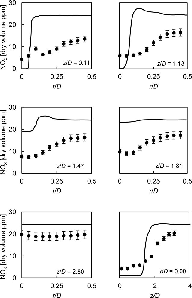
Figure 13. NO_x values at selected local profiles. Comparison between experimental data and AGNES results obtained using an FGM simulation as input, GRI 2.11 and T, velocity direction, Y_H2O, Y_CH4, and Y_O2 as clustering criteria for condition b (ϕ ≅ 0.77).

Additionally, some features should be further investigated. The fact that the GRI 2.11 can be more accurate raises doubts regarding the prompt NO_x formation, as discussed by Perpignan and Rao (2019). The GRI 2.11 is supposedly inferior to its successor, GRI 3.0, but the apparent better representation of the prompt NO_x pathway might be related to different reaction rates in vitiated environments. The chemistry of NO_x formation was shown to be different in previous literature, not only because of thermal NO_x abatement (Nicolle and Dagaut, 2006; Fortunato et al., 2018).

In order to understand what causes the non-monotonic behavior of NO_x, the rates of formation by each pathway were estimated. The rates of the reactions responsible for NO formation at the end of each pathway were taken into account. It is important to highlight that the pathways are not independent and interact with each other. Therefore, isolating their respective contributions is not entirely possible. Nonetheless, the analysis herein performed serves as an indication. The largest source of uncertainty is concerning the thermal and prompt pathways. The N atoms that are products along the prompt pathway tend to react via the second reaction of the Zeldovich pathway (Lefebvre and Ballal, 2010). Therefore, the NO formation coming from the second and third reactions of the Zeldovich pathway was neglected. The thermal NO contribution is considered to be that of the first equation (O + N₂ ↔ NO + N), which is the rate limiting step of the pathway (Glarborg et al., 2018).

As far as the prompt pathway is concerned, the GRI 2.11 mechanism considers the route to follow the HCN → CN → NCO → NO pathway, which was for long believed to be pathway through which the reactions progressed (Lefebvre and Ballal, 2010). Currently, it is known that the NCN route is active instead (Glarborg et al., 2018). In the present analysis, the prompt pathway is considered as it was in the development of GRI 2.11. Therefore, the NO forming reactions shown in Equations (9)–(13) were taken into account to calculate the NO formation rate.

$\begin{array}{ll}\text{N}\text{C}\text{O}+\text{O}\leftrightarrow \text{N}\text{O}+\text{C}\text{O}& (9)\end{array}$

$\begin{array}{ll}\text{N}\text{C}\text{O}+\text{O}\text{H}\leftrightarrow \text{N}\text{O}+\text{H}+\text{C}\text{O}& (10)\end{array}$

$\begin{array}{ll}\text{N}\text{C}\text{O}+{\text{O}}_2\leftrightarrow \text{N}\text{O}+\text{C}{\text{O}}_2& (11)\end{array}$

$\begin{array}{ll}\text{C}\text{H}+\text{N}\text{O}\leftrightarrow \text{H}\text{C}\text{N}+\text{O}& (12)\end{array}$

$\begin{array}{ll}\text{C}\text{H}+\text{N}\text{O}\leftrightarrow \text{H}+\text{N}\text{C}\text{O}& (13)\end{array}$

The contribution of the N₂O pathway was calculated by the NO formation rates of Equations (14)–(16). On Equation (15), it is clear that the N₂O pathway interacts with the prompt pathway via the formation of NCO. That interaction, however, does not directly interfere with the calculation of the NO formation rate, as N₂O and NCO are on opposite sides of the reaction.

$\begin{array}{ll}{\text{N}}_2\text{O}+\text{O}\leftrightarrow 2\text{N}\text{O}& (14)\end{array}$

$\begin{array}{ll}\text{N}\text{C}\text{O}+\text{N}\text{O}\leftrightarrow {\text{N}}_2\text{O}+\text{C}\text{O}& (15)\end{array}$

$\begin{array}{ll}\text{N}\text{H}+\text{N}\text{O}\leftrightarrow {\text{N}}_2\text{O}+\text{H}& (16)\end{array}$

Finally, the NNH pathway was taken into account with the only reaction forming NO in the pathway present in GRI 2.11 (Equation 17).

$\begin{array}{ll}\text{N}\text{N}\text{H}+\text{O}\leftrightarrow \text{N}\text{H}+\text{N}\text{O}& (17)\end{array}$

In Figure 14, a comparison between the NO formation rates for conditions a, b, and e is displayed for the case with GRI 2.11 and Y_O2 included as a clustering criterion. The figure displays the results along an axial line at the radial position r = 15 mm. This position was found to have the highest rates of formation and, therefore, it was selected. Several conclusions can be drawn from this analysis. The first important fact is that thermal NO decreases as ϕ is reduced (going from condition a–f). In fact, the rates of thermal NO reduces as much as 3 orders of magnitude from condition a to f , showing that the contribution of thermal NO cannot explain the overall trend.

FIGURE 14

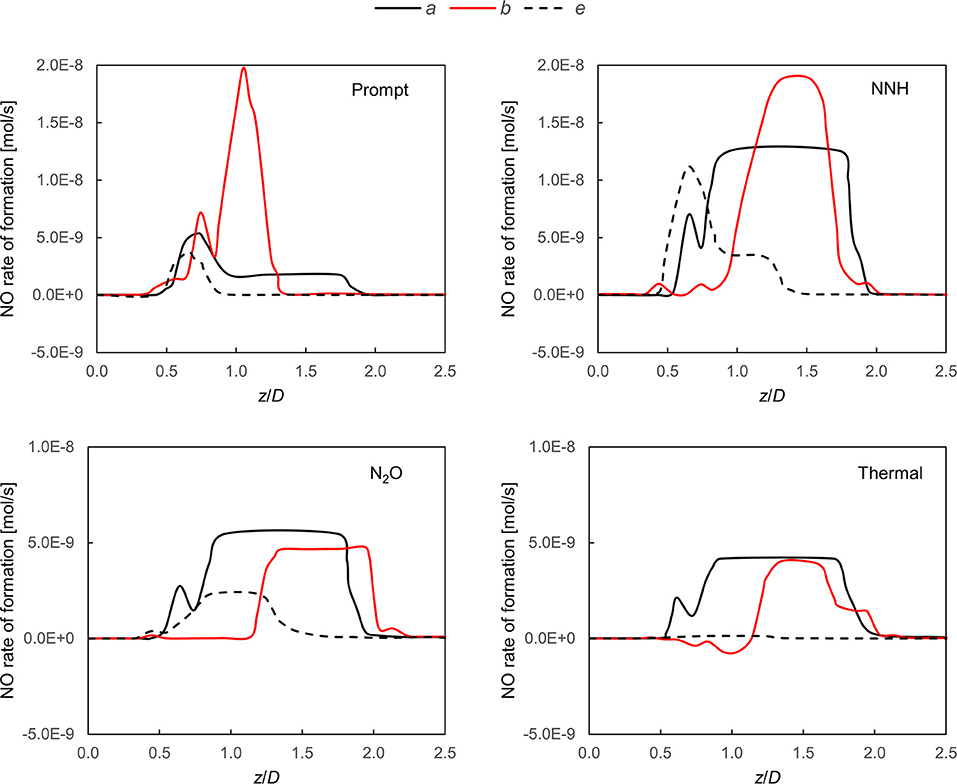
Figure 14. NO formation rates at r = 15 mm along the axial direction for the different formation pathways. Values presented for conditions a (ϕ ≅ 0.91), b (ϕ ≅ 0.77), and e (ϕ ≅ 0.53).

Secondly, the role of the prompt pathway is shown to be important. The rates of NO production by prompt peak for condition b, which explains why this condition has the highest total value of NO_x. Possibly, this peak was predicted for condition b in the simulations while it occurs for condition e according to the experimental data. The prompt pathway was previously shown to be responsible for the peak in NO at lean values for systems operating under FC or with high recirculation (Perpignan et al., 2018b; Perpignan and Rao, 2019).

Thirdly, the role of the NNH pathway is also prominent. Its peak NO formation value is higher at condition b than at condition a. It should be noted that reactions tend to occur further downstream for condition b if compared to the other two conditions. This is an indication of how important the predictions of jet development, recirculation and entrainment coming from the CFD solutions are, since NO formation via pathways other than thermal is dependent on slight variations in composition.

Conclusions and Recommendations

The current work presented CFD and CRN simulations of a combustor developed to investigate FC. The FGM model and the EDM were employed in RANS simulations for simulating several operating conditions of the combustor. The CFD results were post-processed and CRNs were built via clustering of the mesh cells and solved with AGNES.

The following conclusions can be drawn from the study:

• The RANS CFD simulations performed with FGM are able to replicate experimental data to a good extent. The main discrepancies were found near the burner head region.

• CFD simulations performed slightly better for the condition in which a conventional combustion regime was attained (d) if compared to the condition with FC (b).

• The CO emission predictions of all simulations performed with AGNES had a fairly good agreement. The proposed approach can achieve good predictions of CO even with computationally cheap and robust CFD modeling as the EDM.

• The use of AGNES significantly improved the NO_x predictions with respect to CFD, and a reasonable agreement with experiments was achieved.

• Simulations showed that, remarkably, the NO_x is formed in a relatively narrow region (from z/D = 1.5–2.0, approximately).

• The variables chosen as clustering criteria proved to have a significant influence on the obtained results. For a given case, a certain set of criteria could prove to be necessary or optimal with respect to the number of reactors. To the best of our knowledge, this finding has not been previously presented in the literature.

• NO formation in the combustor seems to be dictated by the prompt and NNH pathways. The variation of prompt NO_x is responsible for the non-monotonic behavior of NO_x with ϕ.

Further investigations should be carried out to improve or clarify the following issues:

• The proposed method should be explored further in order to optimize clustering criteria.

• The reproduction of outlet emissions for the employed case may require the use of a CFD model able to perform both in the FC regime as well as in conventional combustion, as different operating conditions result in different combustion regimes.

• The validation and subsequent use of chemical reaction mechanisms for highly vitiated conditions would probably aid the performance of AGNES.

• The assessment on the effect of including turbulent fluctuations on the CRN is recommendable. This can be done by clustering the computational cells based on fluctuation values and/or by employing a Partially Stirred Reactor approach.

• The prompt pathway should be investigated under FC and highly vitiated environments due its key role.

Data Availability Statement

All datasets generated for this study are included in the article.

Author Contributions

AP conceived the idea behind the paper, performed CFD simulations, and took the lead in the writing of the paper. RS wrote the code for AGNES, performed CRN simulations, and actively contributed with the writing. AG supervised the performed worked, was fundamental in discussions about the methods and results, and actively contributed with the writing.

Funding

AP had his PhD research funded by CNPq (National Counsel of Technological and Scientific Development—Brazil) via the Science without Borders program.

Conflict of Interest

The authors declare that the research was conducted in the absence of any commercial or financial relationships that could be construed as a potential conflict of interest.

Acknowledgments

The authors would like to thank CNPq (National Counsel of Technological and Scientific Development—Brazil) support via the Science without Borders program. RS would like to thank Mitsubishi Turbocharger and Engine Europe B.V. (MTEE) for the opportunity of a MSc thesis during which AGNES was developed and Ir. Eline ter Hofstede, R&D Engineer at MTEE, for providing guidance during the project.

References

Benedetto, D., Pasini, S., Falcitelli, M., La Marca, C., and Tognotti, L. (2000). Emission prediction from 3-D completemodelling to reactor network analysis. Combust. Sci. Technol. 153, 279–294. doi: 10.1080/00102200008947265

CrossRef Full Text | Google Scholar

Bowman, C. T., Hanson, R. K., Davidson, D. F., Gardiner W.C. Jr., Lissianski, V., Smith, G. P., et al. Available online at: http://www.me.berkeley.edu/gri_mech/ (accessed February 01, 2019).

Google Scholar

Camargo, J. A., and Alonso, Á. (2006). Ecological and toxicological effects of inorganic nitrogen pollution in aquatic ecosystems: a global assessment. Environ. Int. 32, 831–849. doi: 10.1016/j.envint.2006.05.002

PubMed Abstract | CrossRef Full Text | Google Scholar

Cavaliere, A., and de Joannon, M. (2004). Mild combustion. Prog. Energy Combust. Sci. 30, 329–366. doi: 10.1016/j.pecs.2004.02.003

CrossRef Full Text | Google Scholar

Cuoci, A., Frassoldati, A., Stagni, A., Faravelli, T., Ranzi, E., and Buzzi-Ferraris, G. (2013). Numerical modeling of NO_x formation in turbulent flames using a kinetic post-processing technique. Energy Fuels 27, 1104–1122. doi: 10.1021/ef3016987

CrossRef Full Text | Google Scholar

Ellabban, O., Abu-Rub, H., and Blaabjerg, F. (2014). Renewable energy resources: current status, future prospects and their enabling technology. Renew. Sustain. Energy Rev. 39, 748–764. doi: 10.1016/j.rser.2014.07.113

CrossRef Full Text | Google Scholar

Falcitelli, M., Tognotti, L., and Pasini, S. (2002). An algorithm for extracting chemical reactor network models from CFD simulation of industrial combustion systems. Combust. Sci. Technol. 174, 27–42. doi: 10.1080/713712951

CrossRef Full Text | Google Scholar

Faravelli, T., Bua, L., Frassoldati, A., Antifora, A., Tognotti, L., and Ranzi, E. (2001). A new procedure for predicting NO_x emissions from furnaces. Comput. Chem. Eng. 25, 613–618. doi: 10.1016/S0098-1354(01)00641-X

CrossRef Full Text | Google Scholar

Fichet, V., Kanniche, M., Plion, P., and Gicquel, O. (2010). A reactor network model for predicting NO_x emissions in gas turbines. Fuel 89, 2202–2210. doi: 10.1016/j.fuel.2010.02.010

CrossRef Full Text | Google Scholar

Fortunato, V., Mosca, G., Lupant, D., and Parente, A. (2018). Validation of a reduced NO formation mechanism on a flameless furnace fed with H₂-enriched low calorific value fuels. Appl. Therm. Eng., 144, 877–889. doi: 10.1016/j.applthermaleng.2018.08.091

CrossRef Full Text | Google Scholar

Frassoldati, A., Frigerio, S., Colombo, E., Inzoli, F., and Faravelli, T. (2005). Determination of NO_x emissions from strong swirling confined flames with an integrated CFD-based procedure. Chem. Eng. Sci. 60, 2851–2869. doi: 10.1016/j.ces.2004.12.038

CrossRef Full Text | Google Scholar

Glarborg, P., Miller, J. A., Ruscic, B., and Klippenstein, S. J. (2018). Modeling nitrogen chemistry in combustion. Prog. Energy Combust. Sci. 67, 31–68. doi: 10.1016/j.pecs.2018.01.002

CrossRef Full Text | Google Scholar

Goodwin, D. G., Speth, R. L., Moffat, H. K., and Weber, B. W. (2018). Cantera: An Object-Oriented Software Toolkit for Chemical Kinetics, Thermodynamics, and Transport Processes. Version 2.4.0. Available online at: https://www.cantera.org

Google Scholar

Grewe, V., Dahlmann, K., Matthes, S., and Steinbrecht, W. (2012). Attributing ozone to NO_x emissions: implications for climate mitigation measures. Atmos. Environ. 59, 102–107. doi: 10.1016/j.atmosenv.2012.05.002

CrossRef Full Text | Google Scholar

Hosseini, S. E., and Wahid, M. A. (2013). Biogas utilization: experimental investigation on biogas flameless combustion in lab-scale furnace. Energy Convers. Manag. 74, 426–432. doi: 10.1016/j.enconman.2013.06.026

CrossRef Full Text | Google Scholar

Huang, X., Tummers, M. J., and Roekaerts, D. J. E. M. (2017). Experimental and numerical study of MILD combustion in a lab-scale furnace. Energy Procedia 120, 395–402. doi: 10.1016/j.egypro.2017.07.231

CrossRef Full Text | Google Scholar

International Energy Agency. (2018). World Energy Outlook 2018.

Google Scholar

IPCC (2014). Climate Change 2014: Synthesis Report. Contribution of Working Groups I, II and III to the Fifth Assessment Report of the Intergovernmental Panel on Climate Change, eds Core Writing Team, R. K. Pachauri, and L. A. Meyer. (Geneva: IPCC), 151.

Google Scholar

Kruse, S., Kerschgens, B., Berger, L., Varea, E., and Pitsch, H. (2015). Experimental and numerical study of MILD combustion for gas turbine applications. Appl. Energy 148, 456–465. doi: 10.1016/j.apenergy.2015.03.054

CrossRef Full Text | Google Scholar

Lamouroux, J., Ihme, M., Fiorina, B., and Gicquel, O. (2014). Tabulated chemistry approach for diluted combustion regimes with internal recirculation and heat losses. Combust. Flame 161, 2120–2136. doi: 10.1016/j.combustflame.2014.01.015

CrossRef Full Text | Google Scholar

Lebedev, A. B., Secundov, A. N., Starik, A. M., Titova, N. S., and Schepin, A. M. (2009). Modeling study of gas-turbine combustor emission. Proc. Combust. Inst. 32, 2941–2947. doi: 10.1016/j.proci.2008.05.015

CrossRef Full Text | Google Scholar

Lefebvre, A. H., and Ballal, D. R. (2010). Gas Turbine Combustion: Alternative Fuels and Emissions. Boca Raton, FL: CRC press. doi: 10.1201/9781420086058

CrossRef Full Text | Google Scholar

Lyra, S., and Cant, R. S. (2013). Analysis of high pressure premixed flames using Equivalent Reactor Networks for predicting NO_x emissions. Fuel 107, 261–268. doi: 10.1016/j.fuel.2012.12.066

CrossRef Full Text | Google Scholar

Magnussen, B. F., and Hjertager, B. H. (1976). On mathematical modeling of turbulent combustion with special emphasis on soot formation and combustion. Symp. Int. Combust. 16, 719–729. doi: 10.1016/S0082-0784(77)80366-4

CrossRef Full Text | Google Scholar

Minamoto, Y., Dunstan, T. D., Swaminathan, N., and Cant, R. S. (2013). DNS of EGR-type turbulent flame in MILD condition. Proc. Combust. Inst. 34, 3231–3238. doi: 10.1016/j.proci.2012.06.041

CrossRef Full Text | Google Scholar

Minamoto, Y., and Swaminathan, N. (2014). Scalar gradient behaviour in MILD combustion. Combust. Flame 161, 1063–1075. doi: 10.1016/j.combustflame.2013.10.005

CrossRef Full Text | Google Scholar

Minamoto, Y., Swaminathan, N., Cant, R. S., and Leung, T. (2014). Reaction zones and their structure in MILD combustion. Combust. Sci. Technol. 186, 1075–1096. doi: 10.1080/00102202.2014.902814

CrossRef Full Text | Google Scholar

Monaghan, R. F., Tahir, R., Cuoci, A., Bourque, G., Füri, M., Gordon, R. L., et al. (2012). Detailed multi-dimensional study of pollutant formation in a methane diffusion flame. Energy Fuels 26, 1598–1611. doi: 10.1021/ef201853k

CrossRef Full Text | Google Scholar

Nastasi, B., and Basso, G. L. (2016). Hydrogen to link heat and electricity in the transition towards future Smart Energy Systems. Energy 110, 5–22. doi: 10.1016/j.energy.2016.03.097

CrossRef Full Text | Google Scholar

Nicolle, A., and Dagaut, P. (2006). Occurrence of NO-reburning in MILD combustion evidenced via chemical kinetic modeling. Fuel 85, 2469–2478. doi: 10.1016/j.fuel.2006.05.021

CrossRef Full Text | Google Scholar

Paltsev, S., Sokolov, A., Gao, X., and Haigh, M. (2018) Meeting the Goals of the Paris Agreement: Temperature Implications of the Shell Sky Scenario. Joint Program Report Series Report 330, 10p. Available online at: http://globalchange.mit.edu/publication/16995

Google Scholar

Park, J., Nguyen, T. H., Joung, D., Huh, K. Y., and Lee, M. C. (2013). Prediction of NO x and CO emissions from an industrial lean-premixed gas turbine combustor using a chemical reactor network model. Energy Fuels 27, 1643–1651. doi: 10.1021/ef301741t

CrossRef Full Text | Google Scholar

Perpignan, A. A. V., Rao, A. G., and Roekaerts, D. J. (2018a). Flameless combustion and its potential towards gas turbines. Prog. Energy Combust. Sci. 69, 28–62. doi: 10.1016/j.pecs.2018.06.002

CrossRef Full Text | Google Scholar

Perpignan, A. A. V., and Rao, A. G. (2019). Effects of chemical reaction mechanism and NO_x formation pathways on an inter-turbine burner. Aeronaut. J. doi: 10.1017/aer.2019.12. [Epub ahead of print].

CrossRef Full Text | Google Scholar

Perpignan, A. A. V., Talboom, M. G., Levy, Y., and Rao, A. G. (2018b). Emission modeling of an interturbine burner based on Flameless Combustion. Energy Fuels 32, 822–838. doi: 10.1021/acs.energyfuels.7b02473

PubMed Abstract | CrossRef Full Text | Google Scholar

Pope, S. B. (1978). An explanation of the turbulent round-jet/plane-jet anomaly. AIAA J. 16, 279–281. doi: 10.2514/3.7521

CrossRef Full Text | Google Scholar

Prakash, V., Steimes, J., Roekaerts, D. J. E. M., and Klein, S. A. (2018). “In modelling the effect of external flue gas recirculation on NO_x and CO emissions in a premixed gas turbine combustor with chemical reactor networks,” in Proceedings of ASME Turbo Expo (Oslo). doi: 10.1115/GT2018-76548

CrossRef Full Text | Google Scholar

Ramaekers, W. J. S., Van Oijen, J. A., and De Goey, L. P. H. (2010). A priori testing of flamelet generated manifolds for turbulent partially premixed methane/air flames. Flow Turbul. Combust. 84, 439–458. doi: 10.1007/s10494-009-9223-1

CrossRef Full Text | Google Scholar

Ranzi, E., Frassoldati, A., Grana, R., Cuoci, A., Faravelli, T., Kelley, A. P., et al. (2012). Hierarchical and comparative kinetic modeling of laminar flame speeds of hydrocarbon and oxygenated fuels. Prog. Energy Combust. Sci. 38, 468–501. doi: 10.1016/j.pecs.2012.03.004

CrossRef Full Text | Google Scholar

Sampat, R. P. (2018). Automatic generation of chemical reactor networks for combustion simulations (Master of Sciences Thesis). Delft: Delft University of Technology.

Google Scholar

Scarlat, N., Dallemand, J. F., Monforti-Ferrario, F., and Nita, V. (2015). The role of biomass and bioenergy in a future bioeconomy: policies and facts. Environ. Dev. 15, 3–34. doi: 10.1016/j.envdev.2015.03.006

CrossRef Full Text | Google Scholar

Shih, T. H., Liou, W. W., Shabbir, A., Yang, Z., and Zhu, J. (1995). A new k-ϵ eddy viscosity model for high reynolds number turbulent flows. Comp. Fluids 24, 227–238. doi: 10.1016/0045-7930(94)00032-T

CrossRef Full Text | Google Scholar

Smith, G. P., Golden, D. M., Frenklach, M., Moriarty, N. W., Eiteneer, B., Goldenberg, M., et al. Available online at: http://www.me.berkeley.edu/gri_mech/ (accessed February 01, 2019).

Google Scholar

van Oijen, J. A. (2018). “Modeling of turbulent premixed flames using flamelet generated manifolds,” in Modeling and Simulation of Turbulent Combustion, eds S. De, A. K. Agarwal, S. Chaudhuri, and S. Sen (Singapore: Springer), 241–265. doi: 10.1007/978-981-10-710-3_7

CrossRef Full Text | Google Scholar

van Oijen, J. A., and De Goey, L. P. H. (2000). Modelling of premixed laminar flames using flamelet-generated manifolds. Combust. Sci. Technol. 161, 113–137. doi: 10.1080/00102200008935814

CrossRef Full Text | Google Scholar

Verhoeven, L. M., Ramaekers, W. J. S., Van Oijen, J. A., and De Goey, L. P. H. (2012). Modeling non-premixed laminar co-flow flames using flamelet-generated manifolds. Combust. Flame 159, 230–241. doi: 10.1016/j.combustflame.2011.07.011

CrossRef Full Text | Google Scholar

Veríssimo, A. S., Rocha, A. M. A., and Costa, M. (2011). Operational, combustion, and emission characteristics of a small-scale combustor. Energy Fuels 25, 2469–2480. doi: 10.1021/ef200258t

CrossRef Full Text | Google Scholar

World Health Organization. (2013). Review of Evidence on Health Aspects of Air Pollution–REVIHAAP Project. Copenhagen: World Health Organization.

PubMed Abstract | Google Scholar

Yousefian, S., Bourque, G., and Monaghan, R. F. (2017). “Review of hybrid emissions prediction tools and uncertainty quantification methods for gas turbine combustion systems,” in Proceedings of ASME Turbo Expo (Charlotte, NC).

Google Scholar

Zhou, B., Costa, M., Li, Z., Aldén, M., and Bai, X. S. (2017). Characterization of the reaction zone structures in a laboratory combustor using optical diagnostics: from flame to flameless combustion. Proc. Combust. Inst. 36, 4305–4312. doi: 10.1016/j.proci.2016.06.182

CrossRef Full Text | Google Scholar

Nomenclature