Modeling Vorticity-Driven Wildfire Behavior Using Near-Field Techniques

1. Introduction

Fire spread simulators are an essential component in the assessment of wildfire risk. Given the requisite information on weather, topography and fuels, they provide fire management end-users with a way to map the likely evolution of an active wildfire across a landscape. Fire spread simulators can also be used to evaluate the effectiveness of different suppression options, as part of a technical assessment of individual fires, or they can be used to inform hazard reduction programs (e.g., prescribed burning or mechanical thinning) as part of broader strategic objectives. The effectiveness of a fire spread simulator, however, is critically dependent on: (i) the accuracy of the information that is used as its input; and (ii) the ability of the underpinning fire spread models and propagation algorithms to faithfully represent the main processes driving fire propagation. This second dependence becomes critical when a fire exhibits dynamic behaviors, which arise in response to multi-scale interactions between the fire and the local fire environment, namely the fuel, weather and topography.

In fact, the current suite of operational fire spread simulators (e.g., Phoenix Rapidfire, FARSITE) are poorly suited to modeling dynamic fire propagation. This is mainly due to their reliance on the assumption that a fire will spread at a quasi-steady rate uniquely determined by environmental conditions, and the assumption that different parts of a fire line propagate independently. This latter assumption, for example, is implicit in propagation algorithms such as those based on Huygens' Principle, which is often used in operational fire spread simulators (Finney, 2004; Tolhurst et al., 2008). Given that several modes of dynamic fire propagation are now known to influence the development of a fire, the limitations of current operational fire spread simulators constitute a significant gap in operational capability.

Documented examples of dynamic fire propagation include that exhibited by junction fires (Viegas et al., 2012; Thomas et al., 2017; Raposo et al., 2018), eruptive fires (Viegas and Pita, 2004; Viegas, 2006), and vorticity-driven lateral spread (VLS) (Sharples et al., 2012; Simpson et al., 2013, 2014, 2016). These modes of dynamic fire propagation are driven by complex interactions between the fire and the atmosphere, or between different parts of the fire itself. For example, VLS arises due to wind-terrain-fire interactions that produce vertical vorticity, which rapidly propagates a fire across steep, leeward slopes in a direction nearly perpendicular to the ambient wind direction (Simpson et al., 2013). Figure 1 provides a clear illustration of how a fire burning on a leeward slope can produce pyrogenic vertical vorticity.

FIGURE 1

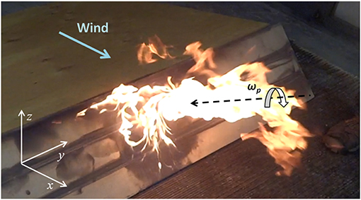
Figure 1. Experimental fire in a wind tunnel showing a fire whirl (vortex) on the leeward slope of an idealized ridge. Note that the vortex is on the left flank of the fire and has components ω_x, ω_z < 0. The pyrogenic vorticity ω_p and its orientation are indicated in the figure. The figure has been adapted from Sharples et al. (2015).

At present it is only possible to accurately model phenomena like VLS using three-dimensional coupled fire-atmosphere models. While such an approach is useful for providing insights into the physical processes that drive such behaviors, their computational cost makes them impractical for operational use. Sharples et al. (2017) modified a two-dimensional fire spread simulator using a specific parameterization that forced the model to emulate the dynamic fire behavior observed in connection with VLS. While this approach permitted faster than real time simulations that captured the main characteristics of VLS and improved the overall accuracy of simulations, the lack of a physical basis for the modifications raises questions about the applicability of such an approach in general.

In this paper we consider a recently developed approach to modeling fire spread (Hilton et al., 2018a), which relaxes the assumptions that rate of spread is quasi-steady and that different parts of a fire burn independently. Although this approach is still manifestly two-dimensional, it has been used to successfully model a number of different modes of dynamic fire spread such as the behavior of junction fires. The two-dimensional nature of the model means that it is able to run much faster than real time, yet is still able to reproduce fire spread features that have previously required fully coupled fire-atmosphere models to resolve. Specifically, we demonstrate how this two-dimensional approach can be extended to accommodate vorticity effects, and use it to model the VLS phenomenon.

We begin by giving a more detailed account of the VLS phenomenon in the next section, before outlining the model extension and its application in a number of specific examples.

2. Vorticity-Driven Lateral Spread

McRae (2004) first noted the presence of atypical modes of fire propagation in multispectral line-scan data from the 2003 Canberra bushfires. These instances, initially referred to as “lee-slope channeling,” are characterized by rapid lateral fire spread across the top of a steep leeward slope in a direction approximately perpendicular to the synoptic wind direction. The upwind edge of the region of lateral spread is constrained by a major break in topographic slope, such as a mountain ridge line. It is also common for the active flaming zone to extend hundreds of meters downwind of the lateral spread region, most likely due to enhanced spotting. Additional features include distinctively darker smoke and vigorous convection associated with the laterally advancing flank of the fire. The rapidity of the lateral spread in a direction that is at odds with the direction a fire would normally be expected to spread, means that this atypical mode of fire propagation can pose a significant danger to firefighter and civilian safety. Indeed, this mode of fire spread has since been implicated in the development of violent pyroconvection (McRae et al., 2015) and in firefighter entrapments (Lahaye et al., 2017).

Subsequent investigation of the phenomenon by Simpson et al. (2013, 2014) using a coupled fire-atmosphere model, indicated that the atypical lateral spread was driven by a three-way interaction between the synoptic winds, the terrain and an active fire. Specifically, it was found that the ambient horizontal vorticity created by flow separation over steep leeward slopes, could be titled and stretched by the rising plume of a fire on the leeward slope to produce strong vertical vorticity, which could then carry the fire laterally across the slope (Sharples et al., 2015). It is of interest to note that the propensity for strong vertical vorticity to form over leeward slopes had been noted much earlier by Countryman (1971). The critical role of pyrogenic vorticity in driving the lateral spread prompted a change in terminology, with the phenomenon subsequently referred to as “vorticity-driven lateral spread” or VLS.

Sharples et al. (2012) identified a number of environmental conditions that were necessary for VLS occurrence. Specifically, they noted that VLS occurrence typically required: a leeward slope angle in excess of about 20–25°; a leeward aspect that aligns to within 30–40° of the wind direction; and wind speeds in excess of about 20 km h⁻¹. In addition, VLS has been observed to occur almost exclusively in heavier fuels (e.g., forest fuels of the order of 15–20 t ha⁻¹). The conditions relating to topography and wind direction can be combined in a simple filter model that identifies parts of the landscape prone to VLS occurrence under a specified wind direction. The VLS filter takes the form of a binary variable, χ, which assumes a value of 1 in regions prone to VLS occurrence and 0 elsewhere. Mathematically, this can be expressed as follows:

$\begin{array}{ll}\chi (\sigma ,\delta )=\{\begin{array}{ll}1,\hfill & \text{if }\frac{{180}^{°}}{\pi }{\tan }^{-1}(||\nabla h||)>\sigma \text{ and }\theta <\delta ;\hfill \\ 0,\hfill & \text{otherwise.}\hfill \end{array}& (1)\end{array}$

Here h is the ground elevation and θ is the angle between the downslope direction and the normalized local wind vector $\widehat{\text{w}}$, defined by:

$\begin{array}{ll}\theta =\{\begin{array}{ll}\frac{{180}^{°}}{\pi }{\cos }^{-1}\left(-\frac{\nabla h·\widehat{\text{w}}}{||\nabla h||}\right),\hfill & \text{if }||\nabla h||>0;\hfill \\ {180}^{°},\hfill & \text{otherwise.}\hfill \end{array}& (2)\end{array}$

The parameters σ and δ, which define the VLS filter, represent threshold values for the topographic slope and θ, respectively. Only parts of the landscape with slopes greater than σ and with θ less than δ are prone to VLS. The values σ = 16° and δ = 40° were found to be appropriate for a digital elevation model of 90 m resolution, but may not be optimal for digital elevation models of different spatial resolution. While this is an important issue, which is currently the focus of ongoing research, it will not affect the results presented in the following sections.

While the VLS filter is useful for identifying slopes that are prone to VLS occurrence, laboratory experiments, wildfire observations and numerical simulations have revealed that the rapid lateral spread associated with VLS really only occurs in a relatively narrow portion of the leeward slope near the top of the hill (Quill and Sharples, 2015; Raposo et al., 2015; Simpson et al., 2016). This region could be better identified using a second-order VLS filter, based on the second-derivative of elevation, but for the idealized cases considered in sections 3 and 4, a crude approximation will suffice. We therefore use a refined version of the first-order filter χ to define VLS prone regions. Specifically, we consider parts of the landscape VLS-prone only if χ = 1 and they are within 100 meters of the ridge line.

Unfortunately, the fact that VLS arises due to a strong coupling between the fire and the atmosphere, means that it is not possible to model VLS using existing two-dimensional fire spread simulators. These simulators, which are based on the notion of a quasi-steady rate of spread and the assumption that different points along a fire line can be treated essentially as independent source fires, are fundamentally unable to account for the dynamic interactions that drive VLS. While it is possible to model the VLS phenomenon using coupled fire-atmosphere models, their computational demand means that they are not feasible as operational tools. Hence, from the operational perspective, the possible effects of VLS on the overall propagation of a wildfire remain unresolved. Indeed, until computational resources evolve to the point that fully coupled fire-atmosphere simulations can be conducted in the order of minutes (rather than hours or days), there appears to be only two possible approaches to incorporating dynamic effects such as VLS in operational fire spread prediction:

(i) Develop parameterizations of the dynamic behaviors, which then facilitate the use of specially tailored sub-models to emulate the observed behaviors; or

(ii) Develop reduced models that capture the main processes governing the dynamic behaviors, but which can be implemented in a highly computationally efficient manner.

Sharples et al. (2017) presented an example of the first of these approaches, using the VLS filter (1) to switch between a standard fire propagation model and one that specifically includes an additional lateral spread component. This model essentially forces the fire to spread laterally in regions identified as prone to VLS, and while this approach was able to improve the accuracy of the fire spread simulator, the lack of a physical basis remains somewhat dissatisfying.

In the remainder of this manuscript we follow the second approach, and discuss a reduced model that accounts for pyroconvective coupling between the fire and the atmosphere in a very straightforward manner.

3. Incorporating Near-Field Effects in Fire Spread Modeling

3.1. Mathematical Model for Local Vorticity Effects

Hilton et al. (2018a) detailed a two-dimensional fire spread model that uses a potential flow formulation to account for local air flows induced by the fire. The so-called “pyrogenic potential” model simulates the pyrogenic air flow close to the ground (mid-flame height), which is assumed to flow horizontally until it reaches the fire, whereupon it moves vertically upwards with the fire's plume. Essentially the model treats the fire as a sink to the induced horizontal flow, the strength of which is related to the intensity of the fire. Once determined, the pyrogenic flow u_p can be added to the ambient wind field, and this net wind field can be used to model the evolution of the fire. In the present work we use a level-set method to simulate the evolution of the fire perimeter, as implemented in the Spark fire simulation framework (Miller et al., 2015).

To determine the pyrogenic flow u_p, we invoke the Helmholtz Decomposition, which states that a twice continuously differentiable vector field with compact support can be expressed as the sum of an irrotational (curl-free) vector field and a solenoidal (divergence-free) vector field (Arfken and Weber, 1999). That is, if a vector field is sufficiently smooth and vanishes as distance r → ∞, then we may write it as the sum of an irrotational vector field ∇ψ and a solenoidal vector field ∇ × η. We refer to ψ as the scalar potential and η as the vector potential.

Considering the flow u_p induced by a fire, it is reasonable to assume that u_p → 0 sufficiently far away from the fire. Hence if we make the assumption that u_p is sufficiently smooth, we can then write:

$\begin{array}{ll}{\text{u}}_p=\nabla \psi +\nabla \times \eta ,& (3)\end{array}$

for some scalar ψ and some vector η. Hilton et al. (2018a) discuss how ψ and η can be determined as solutions of the Poisson equations:

$\begin{array}{ll}{\nabla }^2\psi =\nu ,{\nabla }^2\eta =\omega ,& (4)\end{array}$

where ν = −∂_zu_z, which represents the derivative of the plume updraft, and ω represents sources of vertical, z, vorticity. Once ψ and η are known, the pyrogenic flow u_p can be determined to account for the effects of the fire on the local atmosphere – we refer to these as near-field effects.

In particular, the model can be used to account for potential sources of vertical vorticity via the solenoidal term in (3), reducing the vector Poisson Equation (4) to:

$\begin{array}{ll}{\nabla }^2{\eta }_z={\omega }_z,& (5)\end{array}$

and the resulting flow in the ground plane to:

$\begin{array}{ll}{u}_{px}=\frac{\partial \psi }{\partial x}+\frac{\partial {\eta }_z}{\partial y},u_{py}=\frac{\partial \psi }{\partial y}-\frac{\partial {\eta }_z}{\partial x},& (6)\end{array}$

3.2. Numerical Implementation of Fire Spread

The spread of a fire over a landscape can be modeled using a two-dimensional approach where the fire is represented as an interface between burnt and unburnt regions (Miller et al., 2015). The growth of this interface, or fire perimeter, can be calibrated to data gathered from experimental fires giving an empirical fire spread rate as a function of variables such as fuel type, wind speed and local topography (Sullivan, 2009). The computational representation for the perimeter can be implemented in several forms. Here we use the level set approach to represent the perimeter (Sethian, 1999), in which the signed distance from the perimeter ϕ is updated over time using the level set equation:

$\begin{array}{ll}\frac{\partial \varphi }{\partial t}+s|\nabla \varphi |=0& (7)\end{array}$

where s is the speed normal to the fire perimeter. The perimeter is identified by finding the contour for which ϕ = 0. For the applications in this study a simple first-order rate-of-spread model (Hilton et al., 2016) consisting of a constant outward spread rate, s_c, plus a term depending on the wind field, u was used:

$\begin{array}{ll}s=s_c+max(\text{u}·\widehat{\text{n}},0)& (8)\end{array}$

where $\widehat{\text{n}}$ is the outward normal vector at the perimeter. To couple the pyrogenic and fire spread models we used u = u_a + s_wu_p, where u_a is an ambient wind vector, u_w is the wind vector created by vorticity sources, given in Equation (6), and s_w is an arbitrary constant governing the effect of the vortex-generated wind speed on the fire.

An example simulation using the pyrogenic vector potential coupled to a wildfire spread simulation is shown in Figure 2 with s_c = 0.5 and s_w = 0.5 in Equation (8). These constants were chosen arbitrarily for illustration. The fire was started from a single start point of radius 4 m located 200 m in the horizontal and vertical directions away from a pyrogenic source term. This source term was a single point with ω_z = 5 at the indicated location. No ambient wind speed was used in the simulation with u_a = 0. The resolution was set to 1 m and run for 200 s. The solid black lines show the position of the fire perimeter every 20 s time and the local wind vectors resulting from the pyrogenic model are shown as grayscale arrows. The effect of the vortex point source is to draw the fire perimeter in a circular path due to the resultant circulating flow around the source in the ground plane. The simulation took approximately 15 s to run on a NVidia GTX 1060 graphics processing unit.

FIGURE 2

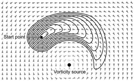
Figure 2. Example application of the pyrogenic potential model with vortex source term to a dynamic wildfire simulation. The black lines show isochrones of a fire perimeter and the arrows show the resultant wind field from the vorticity source.

3.3. Analytical Solution for Vortex Roll Interaction

The key challenge in modeling VLS is to determine a way of translating the ambient horizontal vorticity that forms over a leeward slope due to flow separation, into vertical (pyrogenic) vorticity, ω_z. Specifically, we seek a closed-form solution for the components of the ambient horizontal vortex roll lofted by a buoyant fire plume.

The set-up under consideration is shown in Figure 3, where separation of the flow creates horizontal vorticity over the leeward slope. We require the vortex components ω for the pyrogenic model:

$\begin{array}{ll}\text{u}=\nabla \psi +\nabla \times \eta ,& (9)\end{array}$

where

$\begin{array}{ll}{\nabla }^2\eta =\omega .& (10)\end{array}$

FIGURE 3

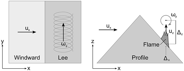
Figure 3. Schematic set-up of model.

We make the following assumptions for the flow dynamics on the lee slope:

(a) The flow can be approximated as steady state using the general steady-state inviscid vorticity equation as the outward spread of the fire is much slower than the wind flow. This is given by (Vallis, 2017):

$\begin{array}{ll}(\text{u}·\nabla )\omega =(\omega ·\nabla )\text{u}+\text{s},& (11)\end{array}$

where u is the flow field, ω is the vorticity vector and s is a source term.

(b) The dominant flow is the vertical lofting flow created by the fire plume; that is, u_z ≫ u_x, u_y. This allows the u_x and u_y components to be neglected in Equation (11).

(c) The flow over the ridge results in a vortex that can be modeled as a prescribed source term. With no loss of generality, this can be aligned with the y-axis so ω_x = 0. The source term is assumed to be a localized line source of the form:

$\begin{array}{l}{s}_y=a\delta (x-{\Delta }_x)\delta (z-{\Delta }_z),\end{array}$

where a is a constant and Δ_x and Δ_z are the x and z coordinates of the vortex line source.

(d) The assumption in the scalar model (Hilton et al., 2018a), ν = −∂_zu_z, is carried over so that u_z = νz with the standard no-flow boundary condition at ground level, u_z = 0 at z = 0.

With these assumptions, Equation (11) reduces to:

$\begin{array}{ll}{u}_z\frac{\partial {\omega }_y}{\partial z}=s_y& (12)\end{array}$

and

$\begin{array}{ll}{\omega }_y\frac{\partial u_z}{\partial y}+{\omega }_z\frac{\partial u_z}{\partial z}=u_z\frac{\partial {\omega }_z}{\partial z}.& (13)\end{array}$

Rewriting Equation (12) using assumptions (c) and (d) gives:

$\begin{array}{ll}\frac{\partial {\omega }_y}{\partial z}=\frac{a}{\nu z}\delta (x-{\Delta }_x)\delta (z-{\Delta }_z).& (14)\end{array}$

Equation (14) can now be solved for ω_y using Laplace transforms. The solution so obtained is:

$\begin{array}{ll}{\omega }_y(z)=\frac{a}{\nu {\Delta }_z}\delta (x-{\Delta }_x)H(z-{\Delta }_z)+b,& (15)\end{array}$

where H(z) is the Heaviside unit step function and b is some constant. This function is sketched in Figure 4—the solution simply has an optional constant vorticity at ground level of magnitude b, undergoes a step change at the line source and is constant thereafter.

FIGURE 4

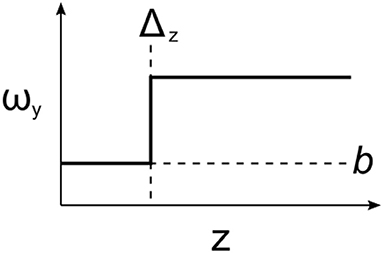
Figure 4. Vorticity ω_y as a function of height z.

Rearranging Equation (13) gives:

$\begin{array}{ll}z\frac{\partial {\omega }_z}{\partial z}-{\omega }_z=\frac{{\omega }_y}{\nu }\frac{\partial u_z}{\partial y},& (16)\end{array}$

and substitution of Equation (15) yields

$\begin{array}{ll}z\frac{\partial {\omega }_z}{\partial z}-{\omega }_z=\frac{1}{\nu }\frac{\partial u_z}{\partial y}\left(\frac{a}{\nu {\Delta }_z}\delta (x-{\Delta }_x)H(z-{\Delta }_z)+b\right).& (17)\end{array}$

This equation has an analytic solution of the form:

$\begin{array}{ll}{\omega }_z(z)=A\delta (x-{\Delta }_x)H(z-{\Delta }_z)\left(\frac{z}{{\Delta }_z}-1\right)-B+Cz,& (18)\end{array}$

where C is some constant and

$\begin{array}{ll}A=\frac{a}{{\nu }^2{\Delta }_z}\frac{\partial u_z}{\partial y},B=\frac{b}{\nu }\frac{\partial u_z}{\partial y}.& (19)\end{array}$

Equation (18) has the form of a ramp function starting at Δ_z. The solution supports a linear term Cz representing the vertical advection of any non-zero ω_z source terms at z = 0. For C = 0 the function is constant for b ≠ 0 and ∂_yu_z ≠ 0. In the simplest possible case of B = 0 and C = 0 the z component of the vorticity will be generated above the line source and linearly scale with height, as shown in Figure 5. Both the ramp function and Cz terms are linearly proportional to z, which is unphysical since ω_z → ∞ as z → ∞. However, these unbounded terms arise from the assumption in the scalar model of ν = −∂_zu_z and realistically Equation (18) only applies to regions below the free stream and above the flame source where the plume is accelerating.

FIGURE 5

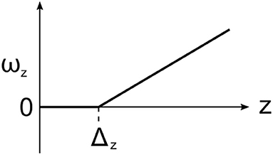
Figure 5. Vorticity ω_z as a function of height z for B = 0 and C = 0.

The pyrogenic model is applied at a nominal mid flame height z₀. At z = z₀ + Δ_z and with b = 0 and C = 0, Equation (18) reduces to:

$\begin{array}{ll}{\omega }_{z0}=k\delta (x-{\Delta }_x)\frac{\partial u_z}{\partial y},& (20)\end{array}$

where:

$\begin{array}{ll}k=\frac{a{z}_0}{{\nu }^2{\Delta }_z^2}& (21)\end{array}$

This result can be generalized to the case of a line source given by a vector equation of the form p + s_xy:

$\begin{array}{ll}{\omega }_{z0}=k\delta (|\text{x}-{\text{x}}^{\prime }|)(\nabla u_z·{\text{s}}_{xy}),& (22)\end{array}$

where x′ is the nearest point on the line source to x. In the case of a plume with constant u_z within a localized region and u_z = 0 outside the region ω_z will only be produced at the intersection of the line source s_xy and the edges of the region. This will give rise to a source term where ∇u_z · s_xy > 0 and a sink where ∇u_z · s_xy < 0 resulting in two counter-rotating vortices, as illustrated in Figure 6.

FIGURE 6

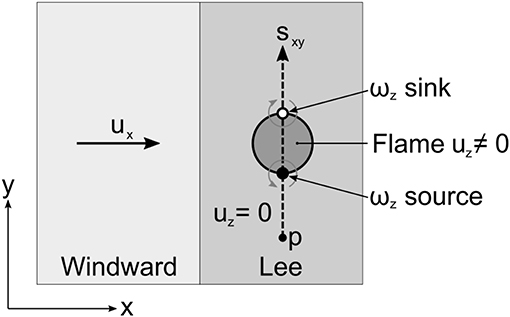
Figure 6. Resultant vorticity in the z direction and circulation in the x-y plane from an idealized plume.

In this case the expression for the vertical vorticity can undergo a final simplification:

$\begin{array}{ll}{\omega }_{z0}=k^{\prime }\delta (|\text{x}-{\text{x}}^{\prime }|)\delta (\varphi )(\widehat{\text{n}}·{\text{s}}_{xy}),& (23)\end{array}$

where $k^{\prime }=u_{z}k$, ϕ is the distance from the fire perimeter and $\widehat{\text{n}}$ is the outward normal of the perimeter.

4. Two-Dimensional Simulation of VLS

In this section we implement the two-dimensional model described in the previous section and evaluate its ability to capture the patterns of dynamic fire propagation associated with VLS. Moreover, we compare the performance of the two-dimensional model with output from a more sophisticated coupled fire-atmosphere model. To this end, we begin by giving a brief overview of the coupled modeling results.

4.1. Coupled Fire-Atmosphere Model

Simpson et al. (2013) conducted idealized large eddy simulations of the VLS phenomenon using the WRF-Fire coupled fire-atmosphere model (Skamarock et al., 2008). The basic configuration considered was an idealized hill with a triangular profile and a height of ~ 1 km. The ridge line at the top of the hill was aligned in a north-south direction. A westerly wind of 20 ms⁻¹ (at the surface) was allowed to flow over the hill, which had a windward slope angle of 20° and a leeward slope angles of 35°. A fire was initiated as a line ignition near the bottom of the leeward slope and allowed to spread. Full details of the simulations are provided by Simpson et al. (2013). It is also of interest to note that Simpson et al. (2015) used similar methods to model a real case, in which VLS had influenced the propagation of the fire, with good agreement between the observed and simulated fire progression.

The idealized simulations were conducted with the fire-atmosphere feedback turned off or turned on. When the fire-atmosphere feedback was turned off, the fire simply propagated back up the leeward slope toward the ridge line and spread laterally at a roughly uniform rate. An example of an uncoupled simulation can be seen in Figures 7A–C. By contrast, when the fire-atmosphere coupling was turned on, the fire spread up the slope until it neared the ridge, at which point it exhibited distinct and rapid lateral growth in a relatively narrow band in the immediate lee of the ridge line. This situation is depicted in Figures 7D–F. These simulations clearly indicate that the rapid lateral spread in the lee of the ridge line associated with VLS is a form of dynamic fire propagation driven by fire-atmosphere coupling.

FIGURE 7

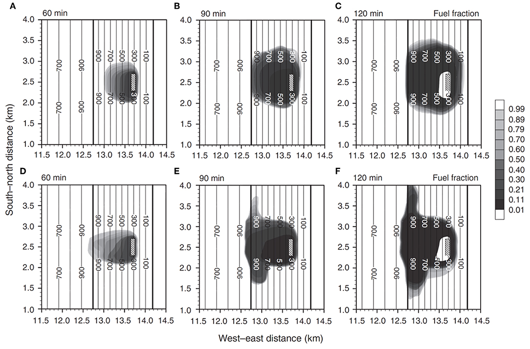
Figure 7. Coupled fire-atmosphere model output of a fire burning on a leeward slope at times of 60, 90, and 120 min into the simulation. Panels (A–C) show model output when the fire-atmosphere coupling is turned off, while panels (D–F) show model output when the fire-atmosphere coupling is turned on. The gray shading indicates the instantaneous fuel fraction remaining. White shading is applied to regions where the fuel fraction remaining is over 99% or under 1%. Terrain contour lines are given at 100-m intervals and the solid black lines represent the ridge line of the hill and the base of the leeward slope. The fire ignition region is indicated by the dash-filled region. The figure has been adapted from Simpson et al. (2013).

It is also important to note that the simulations conducted by Simpson et al. (2013) were computationally intensive, with each 2 h simulation taking around 8–10 h to run on a HPC platform.

4.2. Pyrogenic Potential Model

The pyrogenic potential model was implemented in the Spark framework, a software system for simulating wildfires (Hilton et al., 2018b). Spark consists of a core computational module for simulating the spread of fire over a landscape based the a level set method along with a set of additional modules for simulating additional types of fire behavior, such as terrain effects, firebrand dynamics and near-field effects of the fire on the local atmosphere. The use of a scalar potential to simulate the near-field effect of the plume on the local air flow was presented in Hilton et al. (2018a). As described in section 3 the extension to a vector potential is straightforward, resulting in a vector Poisson equation.

For the purposes of the two-dimensional simulations the horizontal vorticity generated by the flow over the hill was assumed to be static and steady state. This is not a requirement of the model, but simplifies calculations as the assumption of a steady state vortex allows the backwards flow in the lee side of a hill to be imposed as a steady wind condition. The vertical vorticity is assumed to be the dominant component affecting the lateral spread of the fire in the ground plane and is dynamically calculated. The assumption reduced the vector Poisson equation (4) to the scalar Poisson Equation (5). The vertical vorticity in Equation (5) is calculated from Equation (23). The equation is numerically solved using a multigrid method (Hilton et al., 2018b).

A dynamic simulation under the idealized conditions given above is shown in Figure 8. The domain consisted of a ridge 1 km high with a slope of 20° on the windward side and 35° on the lee slope – the same configuration as used by Simpson et al. (2013). The ignition was initiated as a line 400 m in length and 50 m in width perpendicular to the ridge at a distance of 750 m down the leeward slope. The domain size was 5 × 5 km with a simulation resolution of 10 m, and the simulation was run for a period of 2 h. The wind direction was perpendicular to the ridge with a speed was 10 ms⁻¹ on the windward slope. The re-circulation was prescribed by setting the wind speed to -1 ms⁻¹ on the lee slope. The fire rate-of-spread, R, used the Rothermel equation (Rothermel, 1972) with fuel type 13 (Anderson, 1982) with a fuel moisture content of 8%, a fuel load of 13.024 tons acre⁻¹ and a surface to volume ratio of 1159 ft⁻¹. The vorticity was prescribed as a line source with p = (−100, 0), s_xy = (0, 1) and k′ = 2000. Note that the position of the vortex line is consistent with the definition of VLS prone parts of the landscape, as discussed in section 2.

FIGURE 8

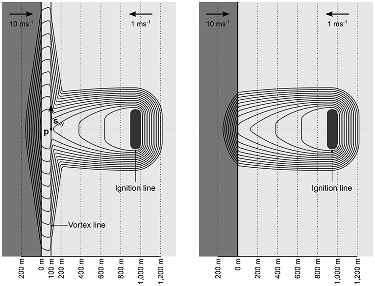
Figure 8. Dynamic calculation in Spark using idealized conditions of B = 0 and C = 0, using the pyrogenic potential model (left) and without (right). The solid lines are fire isochrones at ten minute intervals.

The Dirac function was represented using a smoothed function:

$\begin{array}{ll}\delta (\varphi )=\frac{2ϵ}{{(e^{ϵ\varphi }+e^{-ϵ\varphi })}^2}& (24)\end{array}$

where ϵ = 0.15 is a smoothing length scale, chosen to numerically smooth the Dirac function (Hilton et al., 2018a).

For the case with pyrogenic vorticity, left-hand side of Figure 8, the fire moves up the ridge under the effect of the imposed lee slope wind before spreading laterally along the ridge. The lateral spread occurs along the imposed vortex line. The degree of lateral spread is proportional to the term k′, and the value used in this simulation was manually chosen to match to the physics-based simulations. In the case of no pyrogenic vorticity, right-hand side of Figure 8, the fire moves up the lee slope and stops at the ridge line.

The pyrogenic potential model output compares favorably to the coupled fire-atmosphere model output. In particular, when the effects of pyrogenic vorticity are included, the two-dimensional model is able to produce patterns of fire propagation that are qualitatively similar to that produced by the coupled fire-atmosphere model (compare the left panel of Figure 8 with Figure 7F). Specifically, the two-dimensional model is able to reproduce the rapid lateral spread across the top of the hill in the immediate lee of the ridge line. Likewise, when the effects of pyrogenic vorticity are not included in the two-dimensional model, the model produces results that are qualitatively similar to the uncoupled simulations depicted in Figure 6C.

There are some notable differences between the two-dimensional model output and that of the fully coupled model. In particular, the lateral extent of the fire spread across the lower parts of the leeward slope, which are not prone to vorticity effects, is much less in the two-dimensional model output compared to that of the fully coupled model (even when the coupling is turned off). These differences are likely due to the influence of turbulence, which are not accounted for in the highly idealized two-dimensional pyrogenic potential model simulations.

Using the pyrogenic model imposed a modest computational overhead on the calculation. Using a NVidia GTX 1060 graphics processing unit the 2 h simulation took around 6 s to run with the pyrogenic vortex model and around 1 s without the model.

5. Discussion and Conclusions

Dynamic modes of fire propagation arising from coupling between a fire and the atmosphere pose a significant challenge to two-dimensional fire spread simulators. Currently, such models are not able to accurately account for such behaviors. Here we have presented a new two-dimensional model based on a pyrogenic vector potential formulation that is able to reproduce a specific mode of fire-atmosphere interaction, namely, rapid lateral spread associated with VLS. The model accomplishes this by incorporating near-field effects driven by pyrogenic indrafts and local interaction of the fire with ambient horizontal vorticity. As such, the model can be seen as a “reduced physics” model, in which fire-atmosphere coupling has been greatly simplified. Despite these simplifications, however, the model is able to capture many of the key features observed in connection with VLS and other forms of dynamic fire spread (Hilton et al., 2018a).

The pyrogenic potential model has a significant computational advantage over the fully coupled fire-atmosphere models that have previously been required to accurately model VLS. The pyrogenic potential model took only about 10 s on a standard desktop computer to simulate 2 h of the spread associated with VLS, whereas the fully coupled model required around 8–10 h of to run on a current state-of-the-art high performance computing platform. This increase in computational efficiency could allow the model to be used in scenarios where computational speed is crucial, such as operational fire spread predictions.

Use of the pyrogenic model in operational prediction systems could provide fire managers with the ability to better appreciate the full range of fire behaviors that could be expected, especially under extreme conditions. For example, the VLS phenomenon has been associated with the generation of mass spotting events and the formation of deep flaming zones, which pose a serious threat to firefighter safety and can enhance the likelihood of pyrocumulonimbus development (McRae et al., 2015). This type of modeling capability would therefore provide fire managers with an unprecedented ability to identify regions most at risk to extreme bushfire development and contribute to improvements in firefighter safety.

Although the model presented here constitutes significant progress in our ability to efficiently model dynamic fire propagation, there are still further modeling scenarios that need to be considered, and a number of improvements that could be implemented. For example, the model has been shown to perform reasonably for only a single wind-terrain configuration. Other configurations such as those considered by Raposo et al. (2015) and Simpson et al. (2016) must be considered. It would also be valuable to assess how the model performs against real cases where the effects of VLS were implicated, such as those presented by Quill and Sharples (2015), Simpson et al. (2015), and Sharples et al. (2017). These avenues of inquiry will be pursued in future work.

Data Availability Statement

The raw data supporting the conclusions of this article will be made available by the authors, without undue reservation, to any qualified researcher.

Author Contributions

The study was conceived and designed by both authors. JH conducted the numerical simulations and prepared the figures, with contributions from JS. The paper was written and reviewed by JS and JH.

Funding

This work was supported by funding from the Bushfire and Natural Hazards Cooperative Research Centre for the project Fire coalescence and mass spotfire dynamics: experimentation, modeling and simulation. Part of this work was also performed in the framework of Project Firewhirl, with reference PTDC/EMS-ENE/2530/2014, supported by the Portuguese Foundation for Science and Technology, with National Funds.

Conflict of Interest

The authors declare that the research was conducted in the absence of any commercial or financial relationships that could be construed as a potential conflict of interest.

Acknowledgments

The authors acknowledge the support of the Bushfire and Natural Hazards Cooperative Research Centre. Parts of the research presented was also undertaken with the assistance of resources and services from the National Computational Infrastructure (NCI), which is supported by the Australian Government.

References

Anderson, H. (1982). Aids to Determining Fuel Models for Estimating Fire Behaviour. General Technical Report INT-122, USDA Forest Service, Intermountain Forest and Range Experiment Station.

Google Scholar

Arfken, G. B., and Weber, H. J. (1999). Mathematical Methods for Physicists. San Diego, CA: AAPT.

Google Scholar

Countryman, C. (1971). Fire Whirls…Why, When, and Where. General technical report, USDA Forest Service, Pacific Southwest Forest and Range Experiment Station, Berkeley, CA.

Google Scholar

Finney, M. A. (2004). Farsite: Fire Area Simulator: Model Development and Evaluation. Research paper RMRS-RP-4 Revised, USDA Forest Service, Rocky Mountain Research Station.

Google Scholar

Hilton, J. E., Miller, C., and Sullivan, A. L. (2016). A power series formulation for two-dimensional wildfire shapes. Int. J. Wildland Fire 25, 970–979. doi: 10.1071/WF15191

CrossRef Full Text | Google Scholar

Hilton, J. E., Sullivan, A., Swedosh, W., Sharples, J., and Thomas, C. (2018a). Incorporating convective feedback in wildfire simulations using pyrogenic potential. Environ. Modell. Softw. 107, 12–24. doi: 10.1016/j.envsoft.2018.05.009

CrossRef Full Text | Google Scholar

Hilton, J. E., Sullivan, A. L., Swedosh, W., Cruz, M. G., Plucinski, M. P., Hurley, R. J., et al. (2018b). The Spark Wildfire Prediction System. Coimbra: Imprensa da Universidade de Coimbra.

Google Scholar

Lahaye, S., Sharples, J., Matthews, S., Heemstra, S., and Price, O. (2017). “What are the safety implications of dynamic fire behaviours?” in MODSIM2017, 22nd International Congress on Modelling and Simulation, eds G. Syme, D. Hatton MacDonald, B. Fulton, and J. Piantadosi (Modelling and Simulation Society of Australia and New Zealand), 1125–1130.

Google Scholar

McRae, R. (2004). “The breath of the dragon – observations of the January 2003 ACT bushfires,” in Proceedings of Bushfire 2004 – Earth, Wind & Fire: Fusing the Elements (Adelaide, SA).

Google Scholar

McRae, R., Sharples, J., and Fromm, M. (2015). Linking local wildfire dynamics to pyroCb development. Nat. Hazards Earth Syst. Sci. 15, 417–428. doi: 10.5194/nhess-15-417-2015

CrossRef Full Text | Google Scholar

Miller, C., Hilton, J., Sullivan, A., and Prakash, M. (2015). “Spark–a bushfire spread prediction tool,” in Environmental Software Systems. Infrastructures, Services and Applications. Vol. 448 of IFIP Advances in Information and Communication Technology, eds R. Denzer, R. Argent, G. Schimak, and J. Hřebíček (Springer International Publishing), 262–271.

Google Scholar

Quill, R., and Sharples, J. (2015). “Dynamic development of the 2013 aberfeldy fire,” in MODSIM2015, 21st International Congress on Modelling and Simulation, eds T. Weber, M. McPhee, and R. Anderssen (Modelling and Simulation Society of Australia and New Zealand), 284–290.

Google Scholar

Raposo, J., Cabiddu, S., Viegas, D., Salis, M., and Sharples, J. (2015). Experimental analysis of fire spread across a two-dimensional ridge under wind conditions. Int. J. Wildland Fire 24, 1008–1022. doi: 10.1071/WF14150

CrossRef Full Text | Google Scholar

Raposo, J., Viegas, D., Xie, X., Almeida, M., Figueiredo, A., Porto, L., et al. (2018). Analysis of the physical processes associated with junction fires at laboratory and field scales. Int. J. Wildland Fire 27, 52–68. doi: 10.1071/WF16173

CrossRef Full Text | Google Scholar

Rothermel, R. (1972). “A mathematical model for predicting fire spread in wildland fuels,” Research Paper INT-115 (Ogden, UT: U.S. Department of Agriculture, Intermountain Forest and Range).

Google Scholar

Sethian, J. A. (1999). Level Set Methods and Fast Marching Methods: Evolving Interfaces in Computational Geometry, Fluid Mechanics, Computer Vision, and Materials Science. Cambridge: Cambridge University Press.

Google Scholar

Sharples, J., Kiss, A., Raposo, J., Viegas, D., and Simpson, C. (2015). “Pyrogenic vorticity from windward and lee slope fires,” in MODSIM2015, 21st International Congress on Modelling and Simulation, eds T. Weber, M. McPhee, and R. Anderssen (Gold Coast, QLD: Modelling and Simulation Society of Australia and New Zealand), 291–297.

Google Scholar

Sharples, J., McRae, R., and Wilkes, S. (2012). Wind–terrain effects on the propagation of wildfires in rugged terrain: fire channelling. Int. J. Wildland Fire 21, 282–296. doi: 10.1071/WF10055

CrossRef Full Text | Google Scholar

Sharples, J., Richards, R., Hilton, J., Ferguson, S., Cohen, R., and Thatcher, M. (2017). “Dynamic simulation of the Cape Barren Island fire using the Spark framework,” in MODSIM2017, 22nd International Congress on Modelling and Simulation, eds G. Syme, D. Hatton MacDonald, B. Fulton, and J. Piantadosi (Hobart, TAS: Modelling and Simulation Society of Australia and New Zealand), 1111–1117.

Google Scholar

Simpson, C., Sharples, J., and Evans, J. (2014). Resolving vorticity-driven lateral fire spread using the WRF-fire coupled atmosphere–fire numerical model. Nat. Hazards Earth Syst. Sci. 14, 2359–2371. doi: 10.5194/nhess-14-2359-2014

CrossRef Full Text | Google Scholar

Simpson, C., Sharples, J., and Evans, J. (2015). “WRF-fire simulation of lateral fire spread in the Bendora Fire on 18 January 2003,” in MODSIM2015, 21st International Congress on Modelling and Simulation, eds T. Weber, M. McPhee, and R. Anderssen (Gold Coast, QLD: Modelling and Simulation Society of Australia and New Zealand), 305–311.

Google Scholar

Simpson, C., Sharples, J., and Evans, J. (2016). Sensitivity of atypical lateral fire spread to wind and slope. Geophys. Res. Lett. 43, 1744–1751. doi: 10.1002/2015GL067343

CrossRef Full Text | Google Scholar

Simpson, C., Sharples, J., Evans, J., and McCabe, M. (2013). Large eddy simulation of atypical wildland fire spread on leeward slopes. Int. J. Wildland Fire 22, 599–614. doi: 10.1071/WF12072

CrossRef Full Text | Google Scholar

Skamarock, W., Klemp, J., Dudhia, J., Gill, D., Barker, D., Duda, M., et al. (2008). A Description of the Advanced Research WRF Version. NCAR Technical Note 475, National Center for Atmospheric Research, Boulder, CO.

Google Scholar

Sullivan, A. L. (2009). Wildland surface fire spread modelling, 1990–2007. 3: Simulation and mathematical analogue models. Int. J. Wildland Fire 18, 387–403. doi: 10.1071/WF06144

CrossRef Full Text | Google Scholar

Thomas, C., Sharples, J., and Evans, J. (2017). Modelling the dynamic behaviour of junction fires with a coupled atmosphere–fire model. Int. J. Wildland Fire 26, 331–344. doi: 10.1071/WF16079

CrossRef Full Text | Google Scholar

Tolhurst, K., Shields, B., and Chong, D. (2008). Phoenix: development and application of a bushfire risk management tool. Austral. J. Emerg. Manage. 23:47.

Google Scholar

Vallis, G. K. (2017). Atmospheric and Oceanic Fluid Dynamics. Cambridge: Cambridge University Press.

Google Scholar

Viegas, D. X. (2006). Parametric study of an eruptive fire behaviour model. Int. J. Wildland Fire 15, 169–177. doi: 10.1071/WF05050

CrossRef Full Text | Google Scholar

Viegas, D. X., and Pita, L. P. (2004). Fire spread in canyons. Int. J. Wildland Fire 13, 253–274. doi: 10.1071/WF03050

CrossRef Full Text | Google Scholar

Viegas, D. X., Raposo, J. R., Davim, D. A., and Rossa, C. G. (2012). Study of the jump fire produced by the interaction of two oblique fire fronts. part 1. analytical model and validation with no-slope laboratory experiments. Int. J. Wildland Fire 21, 843–856. doi: 10.1071/WF10155

CrossRef Full Text | Google Scholar