Heat Release Rate Markers for the Adelaide Jet in Hot Coflow Flame

1. Introduction

The Heat Release Rate (HRR) is a key physical quantity in combustion processes. It represents the amount of heat released per unit of time and space due to chemical reactions. Its spatial distribution directly influences important physical phenomena such as flame-turbulence interactions, sound generation and its interaction with flames. This latter may results in combustion instabilities, thus affecting the behavior of practical devices, such as gas turbines (Nikolaou and Swaminathan, 2014).

The mathematical expression of HRR is:

$\begin{array}{ll}HRR={\displaystyle \sum _{\alpha =1}^N}{\stackrel{\cdot }{\omega }}_{\alpha }{h}_{f,\alpha }^0& (1)\end{array}$

where N is the number of species, ${\stackrel{\cdot }{\omega }}_{\alpha }$ is the reaction rate of the α-th chemical species, and $h_{f,\alpha }^0$ is its standard enthalpy of formation. Clearly, a direct measurement of the HRR would involve the accurate determination of a significant number of scalars simultaneously (Nikolaou and Swaminathan, 2014). Due to such a high complexity, it is more practical to measure a quantity that presents some correlation with this rate over the relevant range of flame and flow parameters (Najm et al., 1998b), to qualitatively estimate the local HRR.

Generally, chemiluminescence of natural excited species, e.g., OH*, CH*, (where *denotes an electronically excited state) and Laser-Induced Fluorescence (LIF) techniques (Najm et al., 1998a,b; Paul and Najm, 1998; Röder et al., 2013; Sidey and Mastorakos, 2015) are used to identify the reaction zone and its topology. However, the choice of the scalars able to identify the reaction region can be influenced by the specific chemical-physical behavior of the combustion process, determined in turn both by operative conditions and fuel mixture (Najm et al., 1998a,b; Nikolaou and Swaminathan, 2014). For instance, Vagelopoulos and Frank (2005) showed that the CH marker provides a reasonable correlation with the HRR only for undiluted reactant mixtures with equivalence ratios, ϕ, of 0.8–1.2, whereas Najm et al. (1998a,b) and Paul and Najm (1998) showed that the formyl radical, HCO, is a good HRR-marker for stoichiometric or slightly rich (ϕ = 1.2) methane and dimethyl ether-air laminar flames. Moreover, the flame stretch effects coming from flame-vortex interaction do not significantly influence this correlation (Najm et al., 1998b). According to the authors, the robust correlation between HRR and HCO concentration may be attributed to three main reasons: (1) HCO is a major intermediate species in oxydation of CH₄ to CO₂; (2) its concentration is directly dependent on its production rate; (3) HCO production is directly dependent on the concentration of CH₂O, that in turn directly depends on the reaction CH₃ + O <=> CH₂O + H, which shows the largest fractional influence on heat release rate (Paul and Najm, 1998). Nevertheless, Minamoto and Swaminathan (2014), Mulla et al. (2016), and Nikolaou and Swaminathan (2014) highlighted the difficulty of accurately measuring HCO concentration due to its low signal to noise ratio, thus suggesting to use the more reliable product of OH and CH₂O local signals. Indeed, such species are involved as reactants in HCO formation from formaldehyde through the reaction OH + CH₂O <=> HCO + H₂O. This reconstructed LIF-signal was demonstrated to be a clear HRR-marker for the investigated conditions. Up to now, a wide number of different analysis (Fayoux et al., 2005; Richter et al., 2005; Li et al., 2018) on flame topology has relied on this assumption. Sidey and Mastorakos (2015) compared the presence of OH and OH* with the flame primary heat release region under MILD conditions, suggesting that the sole OH may not be a comprehensive HRR marker for MILD regime.

In more recent studies, Nikolaou and Swaminathan (2014) and Mulla et al. (2016) re-examined the validity of this reaction rate as flame marker for a certain number of combustion conditions. In particular, using Direct Numerical Simulations (DNS) data, they investigated undiluted and diluted methane-air flames, and multicomponent fuel mixtures under both laminar and turbulent conditions. The diluted case operated in Moderate or Intense Low oxygen Dilution (MILD) conditions (Minamoto and Swaminathan, 2014). Remarkable findings shown were: (1) a large fractional contribution of a reaction to the HRR does not automatically imply that this will have a good correlation with the HRR (Nikolaou and Swaminathan, 2014); thus, the rate of the aforementioned reaction, CH₃ + O <=> CH₂O + H, which often shows a high fractional influence on HRR, is not necessarily well correlated with the HRR. (2) HRR correlation is strongly dependent on the equivalence ratio. As a consequence, alternative markers were proposed. The product of H and CH₂O concentrations, corresponding to reaction H + CH₂O <=> HCO + H₂, instead of OH and CH₂O ones was suggested for turbulent MILD and conventional premixed methane-air flames. The viability of H-CH₂O product LIF signal was demonstrated in Mulla et al. (2016).

The aim of this study is to add further understanding on the adequacy of the various HRR markers under diluted condition of a methane/hydrogen-air mixture for both MILD and not-MILD conditions. To this purpose, the widely studied Adelaide Jet in Hot Coflow (JHC) burner (Dally et al., 2002; Medwell et al., 2007; Wang et al., 2011) is modeled following Christo and Dally (2005); Aminian et al. (2012); Parente et al. (2016); Ferrarotti et al. (2019). Firstly, spatial correlations of chemical species and reaction rates with the local HRR are studied. Thence, appropriate combinations of species mole fractions are also taken into consideration and compared with conventional markers.

2. Methodology

2.1. Adelaide Jet in Hot Coflow Burner

The Adelaide JHC (Dally et al., 2002) has been extensively studied and modeled in literature because of its ability to emulate the MILD combustion regime as well as the large number of available experimental data. Hence, it represents a reference test case to validate computational models. For sake of clarity, a sketch of the burner is shown in Figure 1, together with numerical predictions of the OH radical for the two configurations investigated in this work. Inlet conditions are reported in Table 1. A central fuel jet made up of CH₄ and H₂ (50/50 by vol.) issues in a hot coflow (temperature of 1300K), made up of combustion products of fixed CO₂ and H₂O (mass fractions Y_CO2 = 6.5%, Y_H2O = 5.5%) and variable O₂ and N₂, coming from a secondary burner mounted upstream. The JHC burner is placed in a wind tunnel which feeds room temperature air at the same velocity of the coflow. In the configurations of interest for this study, namely HM1 and HM3 of Dally et al. (2002), coflow oxygen concentrations of 3% and 9% by mass, respectively, are considered. The same terminology of Dally et al. (2002) will be used in this paper for these two flames. The strong dilution kept in the HM1 configuration allows to emulate MILD combustion conditions in the first 100 mm of the flame (Medwell et al., 2007). After that, the entrained air from the surroundings changes the flame structure, which becomes closer to a standard diffusion flame, as shown in Figure 1B.

FIGURE 1

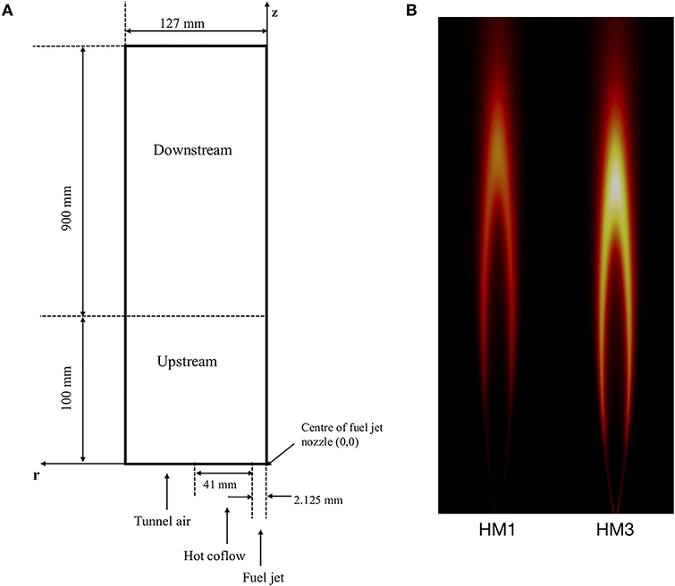
Figure 1. (A) 2D sketch of the Adelaide Jet in Hot Coflow (adapted from Li et al., 2018); (B) Numerical predictions of OH for HM1 and HM3 flames.

TABLE 1

Table 1. JHC inlet velocities and temperatures.

2.2. Numerical Model

Unsteady Favre-Averaged Numerical Simulations (uFANS) were performed using ANSYS Fluent R19.5. A two-dimensional axisymmetric grid, 0.6 m along axial direction and 0.2 m wide, of about 35k quadrilateral cells was employed. Two additional meshes were considered to evaluate the Grid Convergence Index (GCI), which was lower than 3% for temperature and major species. Moreover, a large refinement was set across the reaction zone to well capture gradients of composition and temperature. The standard k-ϵ with the first constant of the dissipation rate equation C_ϵ1 = 1.6 (hence modified for round jets as suggested by Pope, 1978; Christo and Dally, 2005) was chosen as turbulence model. Turbulence-chemistry interactions were modeled using the Partially Stirred Reactor (PaSR) model (Chomiak, 1990; Golovitchev and Chomiak, 2001). As with other reactor based models, the computational cell is split into two zones, one reactive and one in which only mixing occurs. The reactive zone mass fraction is estimated considering both the characteristic chemical and mixing time-scales τ_c and τ_mix:

$\begin{array}{ll}\kappa =\frac{{\tau }_c}{{\tau }_c+{\tau }_{mix}}.& (2)\end{array}$

The approach suggested by Ferrarotti et al. (2019) was used to express τ_mix: the mixing time-scale is proportional to the integral time-scale $\frac{\kappa }{ϵ}$:

$\begin{array}{ll}{\tau }_{mix}=C_{mix}\frac{\kappa }{ϵ}.& (3)\end{array}$

Based on previous studies (Ferrarotti et al., 2019), a constant C_mix of 0.5 was considered. A dynamic approach (Sanders and Gökalp, 1998; Raman and Pitsch, 2007; Ye, 2011; Li et al., 2018; Ferrarotti et al., 2019) was then followed: the mixing time-scale τ_mix is defined based on local properties of the flow field, as it is estimated as the ratio of the mixture fraction variance Z^″2 to the mixture fraction dissipation rate χ:

$\begin{array}{ll}{\tau }_{mix}=\frac{\widetilde{{Z^{″}}^2}}{\tilde{\chi }}.& (4)\end{array}$

Transport equations for the Favre average of the two variables can be written as:

$\begin{array}{ll}\frac{D\bar{\rho }\widetilde{{Z^{″}}^2}}{Dt}=\frac{\partial }{\partial x_j}(\rho (D_m+D_t)\frac{\partial \widetilde{{Z^{″}}^2}}{\partial x_j})+2\rho D_t{(\frac{\partial \tilde{Z}}{\partial x_j})}^2-\rho \tilde{\chi },& (5)\end{array}$

$\begin{array}{l}\frac{D\rho \tilde{\chi }}{Dt}=\frac{\partial }{\partial x_j}(\rho (D_m+D_t)\frac{\partial \tilde{\chi }}{\partial x_j})-C_{D_1}\bar{\rho }\frac{{\tilde{\chi }}^2}{\widetilde{{Z^{″}}^2}}-C_{D_2}\bar{\rho }\frac{\tilde{\chi }\widetilde{ϵ}}{\tilde{\kappa }}\\ +C_{P_1}\frac{\tilde{\chi }}{\widetilde{{Z^{″}}^2}}{P}_f+C_{P_2}\frac{\tilde{\chi }}{\tilde{\kappa }}{P}_k.& (6)\end{array}$

where Z is the mixture fraction, D_t is the turbulent diffusivity, $P_f=-2\bar{\rho }\widetilde{u_k^{″}{Z}^{″}}(\frac{\partial \tilde{Z}}{\partial x_k})$ is the production of scalar fluctuation and $P_k=-\bar{\rho }\widetilde{u_k^{″}{u}_i^{″}}(\frac{\partial \widetilde{U_i}}{\partial x_k})$ is the production of turbulent kinetic energy. The set of coefficients C_P1, C_P2, C_D1, C_D2 used is the one proposed by Ye (2011). The discrete ordinate (DO) method was used to solve the radiative transfer equation, estimating spectral properties of the gaseous medium with the Weighted Sum of Gray Gases Model (WSGGM). Detailed chemistry was taken into account using the GRI2.11 mechanism (Bowman et al., 2020), excluding nitrogen-containing species. A sub-mechanism assembled by Kathrotia et al. (2012) and used also by Doan et al. (2018) was added to the main mechanism, to account for the conventional HRR-marker OH (A²Σ⁺), namely OH*. OH* is generally accepted as a marker for the flame-front structure and heat release rate, therefore its inclusion in the mechanism should enhance the description of the phenomena. This sub-mechanism consists of twelve reactions, whose Arrhenius terms are taken from Kathrotia et al. (2010), Tamura et al. (1998), and Smith et al. (2002). The resulting mechanism contains 32 chemical species and 187 reactions. To reduce the computational time associated to detailed chemistry, the In situ Adaptive Tabulation (ISAT) method by Pope (1997) was adopted with an ISAT tolerance of 10⁻⁵.

2.3. Analysis

HRR, chemical species mole fraction (X_α, where α is the species index) and net reaction rate (${\stackrel{\cdot }{\omega }}_r$, where r is the reaction index) values were sampled along the radial direction at various axial distances from the burner nozzle. Each sampled profile is 50 mm long starting from the burner axis. Obtained data were used to estimate the metric Z(ν) at each axial location as proposed by Nikolaou and Swaminathan (2014), to appreciate how much a scalar ν is representative of the HRR. In particular, Z(ν) for the radial segment s is defined as:

$\begin{array}{ll}{Z}_s(\nu )={\displaystyle \sum _{n=1}^{Np}}{(\frac{|HR{R}_{n,s}|}{ma{x}_s(|HRR|)}-\frac{|{\nu }_{n,s}|}{ma{x}_s(|\nu |)})}^2.& (7)\end{array}$

In the equation above, Np indicates the number of points of the radial segment, max_s(|HRR|) and max_s(ν) are the maximum HRR and ν of that segment, respectively, while ν can be any scalar of interest. For the current case, it is either the mole fraction of the α chemical species X_α, or the reaction rate ${\stackrel{\cdot }{\omega }}_r$. Z_s(ν) was normalized as $Z_s^{+}=100·Z_s/max(Z_s)$, as explained by Nikolaou and Swaminathan (2014). The Z-metric gives an idea on how well a normalized scalar reproduces the spatially matched normalized HRR. At each radius, the lowest values of $Z_s^{+}(\nu )$ identifies the scalars that best correlate with the HRR. It is worth to repeat that the fractional contribution of a reaction to the HRR is not a good way to identify the best HRR markers, whereas the Z-metric is a more rigorous technique, and for this reason was chosen as benchmark for comparison. If the chosen scalar is the net reaction rate, it may have positive and negative contributions to Z, thus giving ambiguous results. However, the top-correlating reactions have either only positive or negative contributions, without influencing the adequacy of the above definition. The results obtained in terms of mole fractions and reactions are presented in Sections 3.1 and 3.2. In Section 3.3, the analysis is also performed substituting to ν appropriate combinations of mole fractions to verify if there are products of species concentrations that may be more suitable for HRR identification.

3. Results and Discussion

3.1. HM1 Case

The simulation results are first confronted with the experimental data from Dally et al. (2002), considering both static and dynamic approaches. Profiles of temperature, OH and CO at the axial locations of 30 and 120 mm, and along the axis are shown in Figure 2 for HM1 (A) and HM3 (B). It can be appreciated how the simulation well reproduce the experimental measurements, as reported in Ferrarotti et al. (2019). Only results from the dynamic approach are presented from here onwards.

FIGURE 2

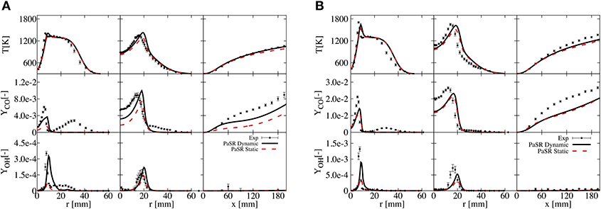
Figure 2. Comparison of T, OH, and CO for static and dynamic PaSR with experimental data at axial locations of 30 and 120 mm and along the axis for HM1 (A) and HM3 (B) configurations.

Figure 3 show $Z_s^{+}(X_{\alpha })$ values for the HM1 case (coflow Y_O2 = 3%), calculated according to Equation (7) when ν = X_α, namely for all the 32 species of the employed mechanism. Furthermore, the product mole fractions of OH and CH₂O proposed by Paul and Najm (1998), and of H and CH₂O suggested by Nikolaou and Swaminathan (2014) are also taken into consideration. Six graphics, one for the respective axial location, x, collect only the first twelve values of $Z_s^{+}(X_{\alpha })$ in ascending order. According to Equation (7), the lowest values are representative of best correlations with HRR. At this point, it is worth to remember that MILD combustion is achieved in the first 100 mm downstream of the burner exit for the HM1 case. After that, the entrained oxygen from the surrounding changes the combustion behavior. As shown in Figure 3A, for x = 30 mm all the species exhibit rather low values of $Z_s^{+}(X_{\alpha })$, as Z⁺ never exceeds 5. O, H, and the conventional HRR-markers OH and OH* provide the lowest values. At this axial location the flame brush is quite thin and the low $Z_s^{+}(X_{\alpha })$ for most of the scalars can be attributed to this reason. Figures 3B,C show a different species ranking for x = 60 mm and x = 90 mm: for the former H and OH* provide lower values of Z⁺, while O and OH are better correlated in the latter. However, at these locations, a clear selection of the best potential HRR markers cannot be made. Besides, $Z_s^{+}(X_{\alpha })$ is generally low (under 10) for all the listed species suggesting that different scalars could be used to detect the reaction zone. Nevertheless, this behavior changes moving further from the jet nozzle: at x = 120 mm (Figure 3D) the gap between the four radicals, O, OH, OH*, H and the others becomes higher while the values of $Z_s^{+}(X_{\alpha })$ grow. This difference is clear in Figure 3E where O, OH, OH* are unambiguously the top-three markers, while H usually presents a slightly lower matching with the HRR. At x = 550 mm (Figure 3F) and higher distances (not reported here) HRR decreases and all the correlations are lost rapidly. It is interesting to note that the formyl radical, HCO, conventionally used as marker with LIF techniques, displays higher values among the correlated species Moreover, contrary to what proposed by Najm et al. (1998b), the product of OH and CH₂O mole fractions does not seem to be a good HRR marker, since its $Z_s^{+}$ is not within the top-five species. This finding may be due to the different chemical pathway followed when methane is diluted with hydrogen and is consistent with results from Kathrotia et al. (2012).

FIGURE 3

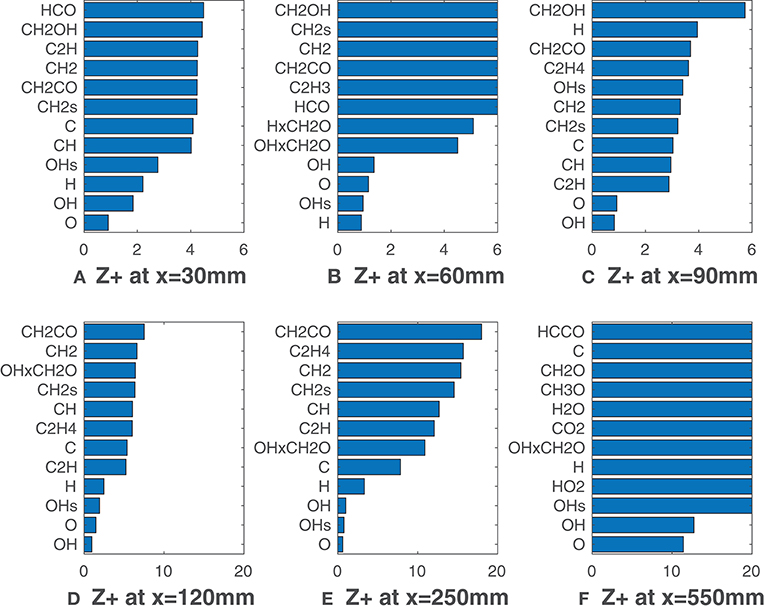
Figure 3. HM1 case: best correlated species at various axial locations. Lower $Z_s^{+}(X_{\alpha })$ values mean better correlation.

Figure 4 adds further insights in this behavior, showing the normalized Z-metric obtained in terms of reactions rates instead of species concentrations. Hence, in Equation (7) the scalar ν is substituted with the kinetic reaction rate, ${\stackrel{\cdot }{\omega }}_r$ (where the subscript r indicates the reaction). What stands out is that several reactions from the added OH(A²Σ⁺) sub-mechanism appear among the top correlated reactions at many axial locations, while the reactions O + CH₃ <=> H + CH₂O, OH + CH₂O <=> HCO + H₂O suggested by Najm et al. (1998b) and Paul and Najm (1998) and the reaction H + CH₂O <=> HCO + H₂ proposed by Nikolaou and Swaminathan (2014) are not present among the ones reported. This may be due to the fuel enrichment with hydrogen, since the cited literature refers to methane-only configurations. This is in line with the previous observations on mole fractions, which do not identify formaldehyde and formyl radical among the markers. Third-body reactions are present in the top ranking positions throughout the flame. The excitation reaction H + O + M <=> M + OH* (Kathrotia et al., 2012), together with CH + O₂ <=> OH* + O, is responsible for the formation of the common HRR marker (Sidey and Mastorakos, 2015; Doan et al., 2018). At x = 60 mm and x = 90 mm (Figures 4B,C) the third-body reaction of oxygen, 2O + M <=> O₂ + M, shows the lowest values of $Z_s^{(+)}({\omega }_r)$ and remains in the top-seven markers till the last sample. A conspicuous number of reactions involving the hydrogen peroxide, H₂O₂, and the hydroperoxyl radical, HO₂, replace the previous ones in the last sampled segment at x = 550 mm (Figure 4F). Moreover, at this axial location, the reactions H + HO₂ <=> 2OH and H + HO₂ <=> O + H₂O do not appear, even though their reaction rates were found to be good HRR indicators by Nikolaou and Swaminathan (2014) for lean to near-stoichiometric methane-air mixtures and especially at low value of HRR.

FIGURE 4

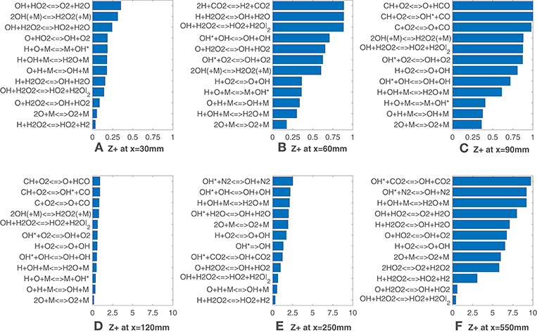
Figure 4. HM1 case: best correlated net reaction rates at various axial locations. Lower $Z_s^{+}({\stackrel{\cdot }{\omega }}_r)$ values mean better correlation.

3.2. Comparison With HM3 Case

Figure 5 reports $Z_s^{+}(X_{\alpha })$ relative to the coflow oxygen concentration of 9%, i.e., HM3 flame. With this configuration the flame is visible since its beginning (Figure 1B), and MILD conditions are not reached. Unlike Figures 3A–D, O, OH, OH* radicals show unambiguously greater correlation with HRR if compared to the other species. O and OH present slightly higher $Z_s^{+}(X_{\alpha })$-values throughout the entire domain. As previously underlined, at long distances HRR decades and $Z_s^{+}(X_{\alpha })$ increases fast for all the species. It is interesting to note that this last phenomena emerges a bit before if compared to the HM1 case. Indeed, in the HM1 configuration combustion is somewhat slowed down due to MILD conditions. This leads to a slightly longer flame for Y_O2 = 3%, explaining why the correlations drop down later with respect to the HM3 case. The product of OH and CH₂O mole fractions appears as well in Figure 5, always having a higher $Z_s^{+}(X_{\alpha })$ value. It is clear that the influence of oxygen concentration plays a significant role in determining the best HRR-markers. For the HM3 case the distinction between the top three markers O, OH, OH* and the others is noticeable from the beginning of the combustion process, whereas, for the 3% coflow case, this distinction becomes clearer only downstream of 100 mm of flame, due to the higher level of entrained oxygen from surroundings.

FIGURE 5

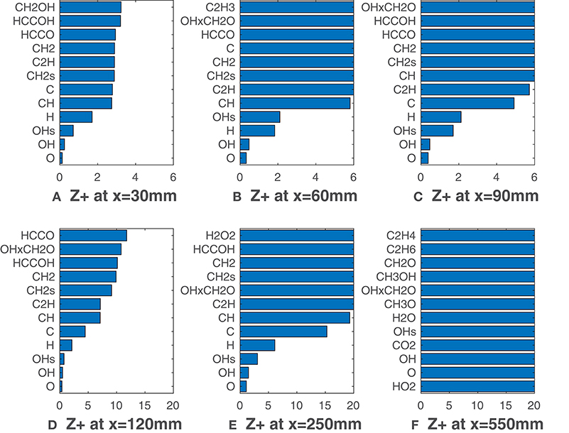
Figure 5. HM3 case: best correlated species at various axial locations. Lower $Z_s^{+}(X_{\alpha })$ values mean better correlation.

Looking now at Figure 6, it is interesting to note that values of $Z_s^{+}({\stackrel{\cdot }{\omega }}_r)$ are generally lower up to 90 mm if compared with the HM1 case. The OH* formation reaction appears again as a good indicator of heat release as several reactions from the sub-mechanism are listed. Also in this case, for x = 250 mm and x = 550 mm (Figures 6E,F), reactions involving hydroperoxyl radical show a very good agreement with the HRR. In the latter, OH + H2O2 <=> HO2 + H2O and O + H2O2 <=> OH + HO2 cover the first positions, suggesting that their rates could be good HRR markers at this location with the 9% coflow oxygen concentration.

FIGURE 6

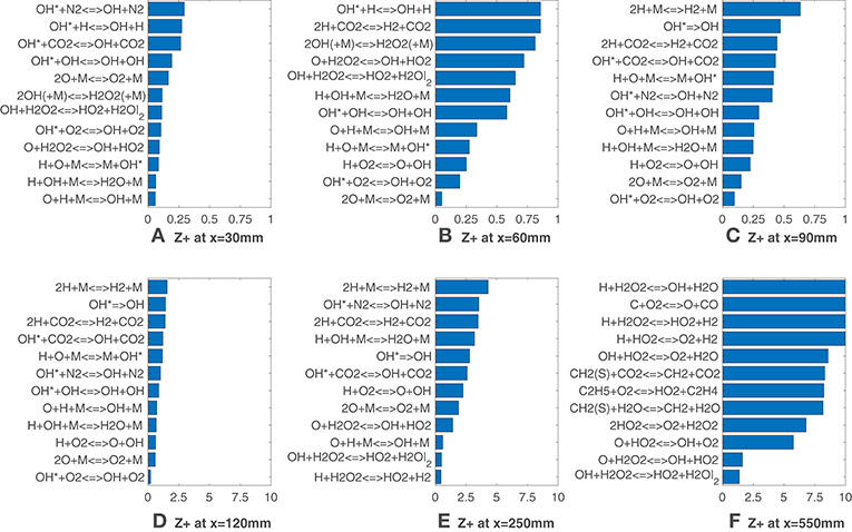
Figure 6. HM3 case: best correlated net reaction rates at various axial locations. Lower $Z_s^{+}({\stackrel{\cdot }{\omega }}_r)$ values mean better correlation.

3.3. Combinations of Mole Fractions

Figures 7, 8 report $Z_s^{+}(\nu )$ calculated substituting species mole fractions X_α and their combinations to ν. It is noteworthy that several combinations present values lower than the lowest ones recorded in Figures 3, 5. The product of O and OH shows a very good agreement with the HRR and is the solution of choice till x = 120 mm (Figure 7). This notable results may suggest that for MILD combustion under the conditions of interest, an appropriate combination of species can identify the reaction zone more precisely than a single species, thus with less uncertainty on the choice of the right scalar. Just above the combination OxOH (here x is the product symbol), combinations of H, O, OH and OH* show also a very good correlation metric. At higher distances, combinations of these 3 radicals with the major species H₂O and CO₂ are ranked first. As expected, this change occurs first for the HM3 configuration (Figure 8).

FIGURE 7

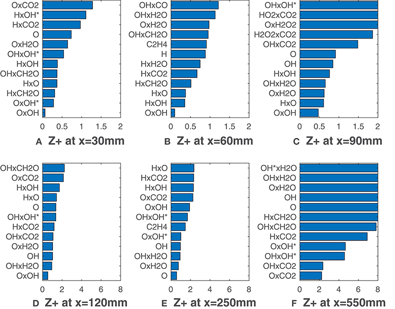
Figure 7. HM1 case: best correlated markers at various axial locations. Lower $Z_s^{+}(\nu )$ values mean better correlation. Here ν comprehends both X_α and their combinations.

FIGURE 8

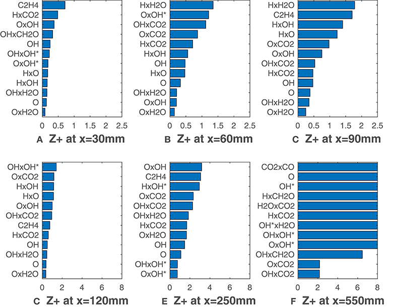
Figure 8. HM3 case: best correlated markers at various axial locations. Lower $Z_s^{+}(\nu )$ values mean better correlation. Here ν comprehends both X_α and their combinations.

The distributions of HRR, mole fraction and combinations are reported and compared in Figure 9. The 6 graphics correspond to 3 positions of the 2 cases studied, i.e., x = 60 mm, x = 120 mm and x = 550 mm, respectively. Only radial profiles of the top-two species and the top-two combinations are drawn together with the HRR. All these scalars are normalized with respect to their own maximum. It is worth noting that both species mole fractions and combinations capture the HRR peak very well in Figures 9A,B,D,E. The main difference is associated to the tails of the curves, for low values of HRR. In particular, using the mole fraction products allows to have a higher correlation in these branches and capture the near-zero HRR behavior. This might also suggest a good detection of local extinction. Different considerations should be done for Figures 9C,F. At x = 550 mm, the HRR curve is wider and, as stated previously, the sole species are not a very good HRR marker, especially for the HM3 case.

FIGURE 9

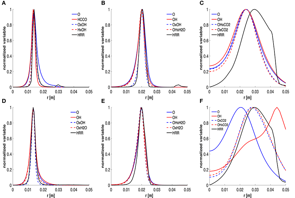
Figure 9. Trends of normalized HRR, top-two mole fractions and combinations at 60 (A,D), 120 (B,E) and 550 (C,F) mm, respectively. First and second row refer to the HM1 and HM3 cases, respectively.

Looking to the contour plots (Figure 10) reported as a qualitative example, it is possible to identify the 3 zones previously underlined. Two black dotted lines divide this zones at x = 150 mm and x = 450 mm. For each part, the best HRR marker combination is reported.

FIGURE 10

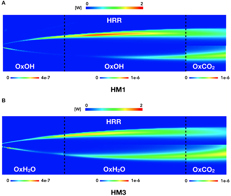
Figure 10. HM1 and HM3 contour plots of HRR compared to species products contours. The three zones are split as follows: from 0 to 150 mm, from 150 to 450 mm, and from 450 to 550 mm.

4. Conclusion

The choice of the right HRR marker is fuel-mixture specific and depends also on operative conditions. Therefore, the applicability of conventional HRR markers is not universal and should be tested for different flame configurations. To further investigate the applicability of the different available markers, numerical simulations of the Adelaide JHC were carried out with detailed chemistry, including the excited species OH*. The interesting feature of the JHC is the possibility to module oxygen dilution and the change in combustion behavior observed when the entrained oxygen from surroundings changes the flame from invisible to visible. Hence, correlations between HRR and both species mole fractions and reaction rates were investigated at various axial locations along the radial direction for two level of coflow oxygen mass fractions, 3% and 9%.

In summary, in a clear distinction among $Z_s^{+}(X_{\alpha })$ values cannot be made for the HM1 case in the first 120 mm of flame. In this range the radical OH is always one of the four top markers (Figure 3). Further downstream from the burner, the top-three markers are O, OH, OH* radicals. The reaction rates that better correlate with the HRR are shown to belong mostly to reactions of the OH* sub-mechanism and involve primarily these radicals together with other species such as H, O₂, HO₂, H₂O₂, H₂O, CO, CO₂. Some of these appearing only at high axial locations. For the HM3 configuration, a very good agreement between the top-three radicals O, OH, OH* and the HRR was found right from the first axial location (Figure 5), suggesting that a higher oxygen level allows better correlation with the HRR. This is in line with the change in the results of the HM1 case, since beyond x = 100 mm, the entrained air increase the available oxygen for the flame (Dally et al., 2002; Medwell et al., 2007). With regard to the most correlated reaction rates, their relative reactions involve again the aforementioned 10 species.

Even though conventional HRR markers such as OH and OH* perform well along most of the flame, a better detection of the reaction zone may be achieved using appropriate combinations of species. Considering the change of the combustion behavior due to the entrained oxygen from the air stream, different parts of the flame should be detected by different markers. For the HM1 case, the combination of O and OH mole fractions seems to be the right choice for the MILD region while beyond x = 150 mm, the HRR is well captured by the product OxCO₂, for both the configurations. Finally, only in the region far from the nozzle, i.e., the last 150 mm of the studied domain, the low and wide values of HRR are better captured by combinations of O and OH with carbon dioxide.

The applicability of these markers for other conditions and fuel mixtures will be subject of future studies.

Data Availability Statement

All datasets generated for this study are included in the article.

Author Contributions

MF carried out the numerical simulations and the post-processing, and lead the manuscript writing. RA and DB contributed to the CFD simulations and paper writing. CG and AP supervised the work, critically discussed the results, and contributed to the writing.

Funding

This project has received funding from the European Research Council (ERC) under the European Union's Horizon 2020 research and innovation programme under grant agreement no. 714605. MF wishes to thank the Fonds de la Recherche Scientifique FNRS Belgium for financing his research.

Conflict of Interest

The authors declare that the research was conducted in the absence of any commercial or financial relationships that could be construed as a potential conflict of interest.

Acknowledgments

The authors thank B. B. Dally at University of Adelaide for granting access to the experimental data.

References

Aminian, J., Galletti, C., Shahhosseini, S., and Tognotti, L. (2012). Numerical investigation of a mild combustion burner: analysis of mixing field, chemical kinetics and turbulence-chemistry interaction. Flow Turbul. Combust. 88, 597–623. doi: 10.1007/s10494-012-9386-z

CrossRef Full Text | Google Scholar

Bowman, C. T., Hanson, R. K., Davidson, D. F., Gardiner, W. C. Jr., Lissianski, V., Smith, G. P., et al. (2020). Gri 2.11 Mechanism. Available online at: http://www.me.berkeley.edu/gri_mech/

Google Scholar

Chomiak, J. (1990). Combustion: A Study in Theory, Fact and Application. New York, NY: Abacus Press; Gorden and Breach Science Publishers.

Google Scholar

Christo, F., and Dally, B. (2005). Modeling turbulent reacting jets issuing into a hot and diluted coflow. Combust. Flame 142, 117–129. doi: 10.1016/j.combustflame.2005.03.002

CrossRef Full Text | Google Scholar

Dally, B., Karpetis, A., and Barlow, R. (2002). Structure of turbulent non-premixed jet flames in a diluted hot coflow. Proc. Combust. Inst. 29, 1147–1154. doi: 10.1016/S1540-7489(02)80145-6

CrossRef Full Text | Google Scholar

Doan, N., Swaminathan, N., and Minamoto, Y. (2018). Dns of mild combustion with mixture fraction variations. Combust. Flame 189, 173–189. doi: 10.1016/j.combustflame.2017.10.030

CrossRef Full Text | Google Scholar

Fayoux, A., Zähringer, K., Gicquel, O., and Rolon, J. (2005). Experimental and numerical determination of heat release in counterflow premixed laminar flames. Proc. Combust. Inst. 30, 251–257. doi: 10.1016/j.proci.2004.08.210

CrossRef Full Text | Google Scholar

Ferrarotti, M., Li, Z., and Parente, A. (2019). On the role of mixing models in the simulation of mild combustion using finite-rate chemistry combustion models. Proc. Combust. Inst. 37, 4531–4538. doi: 10.1016/j.proci.2018.07.043

CrossRef Full Text | Google Scholar

Golovitchev, V., and Chomiak, J. (2001). “Numerical modeling of high temperature air flameless combustion,” in Proceedings of the 4th International Symposium on High Temperature Air Combustion and Gasification (HiTACG) (Rome), 27–30.

Google Scholar

Kathrotia, T., Fikri, M., Bozkurt, M., Hartmann, M., Riedel, U., and Schulz, C. (2010). Study of the h+o+m reaction forming OH*: Kinetics of OH* chemiluminescence in hydrogen combustion systems. Combust. Flame 157, 1261–1273. doi: 10.1016/j.combustflame.2010.04.003

CrossRef Full Text | Google Scholar

Kathrotia, T., Riedel, U., Seipel, A., Moshammer, K., and Brockhinke, A. (2012). Experimental and numerical study of chemiluminescent species in low-pressure flames. Appl. Phys. B 107, 571–584. doi: 10.1007/s00340-012-5002-0

CrossRef Full Text | Google Scholar

Li, Z., Ferrarotti, M., Cuoci, A., and Parente, A. (2018). Finite-rate chemistry modelling of non-conventional combustion regimes using a partially-stirred reactor closure: combustion model formulation and implementation details. Appl. Energy 225, 637–655. doi: 10.1016/j.apenergy.2018.04.085

CrossRef Full Text | Google Scholar

Medwell, P. R., Kalt, P., and Dally, B. (2007). Simultaneous imaging of oh, formaldehyde, and temperature of turbulent nonpremixed jet flames in a heated and diluted coflow. Combust. Flame 148, 48–61. doi: 10.1016/j.combustflame.2006.10.002

CrossRef Full Text | Google Scholar

Minamoto, Y., and Swaminathan, N. (2014). Scalar gradient behaviour in mild combustion. Combust. Flame 161, 1063–1075. doi: 10.1016/j.combustflame.2013.10.005

CrossRef Full Text | Google Scholar

Mulla, I., Dowlut, A., Hussain, T., Nikolaou, Z., Chakravarthy, S., Swaminathan, N., et al. (2016). Heat release rate estimation in laminar premixed flames using laser-induced fluorescence of ch2o and h-atom. Combust. Flame 165, 373–383. doi: 10.1016/j.combustflame.2015.12.023

CrossRef Full Text | Google Scholar

Najm, H., Knio, O., Paul, P., and Wyckoff, P. (1998a). A study of flame observables in premixed methane - air flames. Combust. Sci. Technol. 140, 369–403. doi: 10.1080/00102209808915779

CrossRef Full Text | Google Scholar

Najm, H., Paul, P., Mueller, C., and Wyckoff, P. (1998b). On the adequacy of certain experimental observables as measurements of flame burning rate. Combust. Flame 113, 312–332. doi: 10.1016/S0010-2180(97)00209-5

CrossRef Full Text | Google Scholar

Nikolaou, Z., and Swaminathan, N. (2014). Heat release rate markers for premixed combustion. Combust. Flame 161, 3073–3084. doi: 10.1016/j.combustflame.2014.05.019

CrossRef Full Text | Google Scholar

Parente, A., Malik, M., Contino, F., Cuoci, A., and Dally, B. (2016). Extension of the eddy dissipation concept for turbulence/chemistry interactions to mild combustion. Fuel 163, 98–111. doi: 10.1016/j.fuel.2015.09.020

CrossRef Full Text | Google Scholar

Paul, P., and Najm, H. (1998). Planar laser-induced fluorescence imaging of flame heat release rate. Symp. (Int.) Combust. 27, 43–50. doi: 10.1016/S0082-0784(98)80388-3

CrossRef Full Text | Google Scholar

Pope, S. (1978). An explanation of the turbulent round-jet/plane-jet anomaly. AIAA J. 16, 279–281. doi: 10.2514/3.7521

CrossRef Full Text | Google Scholar

Pope, S. (1997). Computationally efficient implementation of combustion chemistry using in situ adaptive tabulation. Combust. Theory Model. 1, 41–63. doi: 10.1080/713665229

CrossRef Full Text | Google Scholar

Raman, V., and Pitsch, H. (2007). A consistent LES/filtered-density function formulation for the simulation of turbulent flames with detailed chemistry. Proc. Combust. Inst. 31, 1711–1719. doi: 10.1016/j.proci.2006.07.152

CrossRef Full Text | Google Scholar

Richter, M., Collinm, R., Nygren, J., Aldeacute, M., Hildingsson, N., and Johansson, B. (2005). Studies of the combustion process with simultaneous formaldehyde and OH PLIF in a direct-injected hcci engine. JSME Int. J. Ser. B Fluids Ther. Eng. 48, 701–707. doi: 10.1299/jsmeb.48.701

CrossRef Full Text | Google Scholar

Röder, M., Dreier, T., and Schulz, C. (2013). Simultaneous measurement of localized heat-release with OH/CH2O-LIF imaging and spatially integrated OH* chemiluminescence in turbulent swirl flames. Proc. Combust. Inst. 34, 3549–3556. doi: 10.1016/j.proci.2012.06.102

CrossRef Full Text | Google Scholar

Sanders, J., and Gökalp, I. (1998). Scalar dissipation rate modelling in variable density turbulent axisymmetric jets and diffusion flames. Phys. Fluids 10, 938–948. doi: 10.1063/1.869616

CrossRef Full Text | Google Scholar

Sidey, J., and Mastorakos, E. (2015). Visualization of mild combustion from jets in cross-flow. Proc. Combust. Inst. 35, 3537–3545. doi: 10.1016/j.proci.2014.07.028

CrossRef Full Text | Google Scholar

Smith, G., Luque, J., Park, C., Jeffries, J., and Crosley, D. (2002). Low pressure flame determinations of rate constants for OH(A) and CH(A) chemiluminescence. Combust. Flame 131, 59–69. doi: 10.1016/S0010-2180(02)00399-1

CrossRef Full Text | Google Scholar

Tamura, M., Berg, P., Harrington, J., Luque, J., Jeffries, J., Smith, G., et al. (1998). Collisional quenching of CH(A), OH(A), and NO(A) in low pressure hydrocarbon flames. Combust. Flame 114, 502–514. doi: 10.1016/S0010-2180(97)00324-6

CrossRef Full Text | Google Scholar

Vagelopoulos, C., and Frank, J. (2005). An experimental and numerical study on the adequacy of CH as a flame marker in premixed methane flames. Proc. Combust. Inst. 30, 241–249. doi: 10.1016/j.proci.2004.08.243

CrossRef Full Text | Google Scholar

Wang, F., Mi, J., Li, P., and Zheng, C. (2011). Diffusion flame of a CH4/H2 jet in hot low-oxygen coflow. Int. J. Hyd. Energy 36, 9267–9277. doi: 10.1016/j.ijhydene.2011.04.180

CrossRef Full Text | Google Scholar

Ye, I. (2011). Investigation of the scalar variance and scalar dissipation rate in URANS and LES (Ph.D. thesis), University of Waterloo, Waterloo, ON, Canada.

Google Scholar