Multi-Scale Surface Roughness Optimization Through Genetic Algorithms

1. Introduction

It is well-established in the literature that surface topology and texture are important for enhancing the tribological behavior of contacts. Therefore, optimization of topological features is considered as a research topic of paramount interest for industrial applications. For instance, optimization of the shape and position of periodic grooved textures has been investigated in Buscaglia et al. (2007) in relation to lubrication. Even more ambitious are the recent attempts to tailor roughness of engineering surfaces by controlling end-milling operations, as discussed in Zhang et al. (2007), or by cutting techniques as in Nouari et al. (2018). Artificial intelligence based on genetic algorithms (Zain et al., 2008) and artificial neural networks (Moghri et al., 2014) have been recently exploited to control milling operations and surface roughness manufacturing by material removal. As another strategy, additive manufacturing (Brettel et al., 2014) is opening new perspectives to produce surfaces with specified roughness (see e.g., Farina et al., 2016; Ko et al., 2019; Wüst et al., 2020).

In addition to tribology, the role of an interface between material constituents/phases is becoming progressively dominant over the one of bulk properties, thanks to the increasing trend in the miniaturization of components, and to the significant progress in the design of mechanical systems and materials, starting from the sub-micrometer scale. The interface has very different properties than the bulk, and is important in a variety of mechanical, physical, and chemical processes. Interfaces can have significant effects also on the properties of composite materials (Moroni et al., 2013; Guo et al., 2014, 2017; Kwon et al., 2019). Consequently, industrial applications often require the design of surface textures able to achieve given target responses and/or to enable rapid manufacturing and morphology changes for in-line control of mechanical components, as in Bora et al. (2005) for Micro-Electro-Mechanical Systems (MEMS). Nature is also offering interesting perspectives for the identification of optimal surface topologies for selected applications, see e.g., the successful attempts to create artificial super-adhesives like Gecko's pads (Sherge and Gorb, 2001; Gao et al., 2005; Nosonovsky and Bushan, 2008).

In the present study, a theoretical multi-scale description of roughness is considered in relation to the Multivariate Weierstrass-Mandelbrot (MWM) function as a model for a fractal rough profile (Cinat et al., 2019). The aim of the research is to establish a mathematical and a computational framework for the robust identification of the profile model parameters that lead to identified topologies whose contact response is matching any requested real contact area-load and contact conductance-load curves that can be specified by the user. Although the authors are aware that not all the natural and manufactured surfaces do obey to the fractal scaling, as pointed out by Carr and Benzer (1991), Wen and Sinding-Larsen (1997), Borri and Paggi (2015), Xiaohan et al. (2017), and Gujrati et al. (2018), the choice here is motivated by the fact that the MWM function has been widely studied in relation to contact mechanics, and, for instance, we expect to find that optimization in the low frequency range is the major concern for controlling the thermal/electric contact conductance, while fine scale features are governing the real area of contact (see e.g., Ciavarella et al., 2000, 2004; Paggi and Barber, 2011). However, it has to be highlighted that, although the MWM model is herein adopted for validating identification predictions in relation to benchmark results established in the literature, the overall proposed computational procedure can be applied also to other profile or surface models as well, without specific restrictions.

Motivated by an analogy with biology, the expression surface roughness genome is herein used to denote the ensemble of parameters, the genes, associated with the set of elementary waves that describes the main features of roughness over multiple length scales. Although such a terminology imported from biology is not usually adopted in the contact mechanics community, it is introduced here for its common use in the research area of genetic algorithms. Within this framework, we optimize the parameters above to identify a suitable genome that produces a rough profile having a frictionless elastic normal contact mechanics response close to a requested target one. To achieve this goal, we propose various genetic algorithms, combining mechanical considerations and suitable optimization tools. The contact problem is solved in terms of the boundary element method (BEM) (Vakis et al., 2018; Paggi and Hills, 2020), based on the formulation validated in Bemporad and Paggi (2015). See also Bemporad and Paggi (2015) for a wide comparison of other BEM techniques that could also be effectively applied to solve the same contact problem.

Regarding the genetic algorithm research contribution, differently from the previous publication by Cinat et al. (2019) where a single algorithm was proposed to achieve that task, here we propose an extensive numerical comparison of the performance of various algorithms with clear distinct features.

This article is structured as follows. In section 2, we describe the normal contact problem, the surface roughness genome, the features of a single length scale of roughness, and the roughness reconstruction over multiple length scales. In section 3, we propose three genetic algorithms, whose aim is to generate prototype profiles able to achieve given target contact mechanics responses. In section 4, the effectiveness of these algorithms is tested and discussed through a representative example, based on an artificial genome database. Finally, section 5 concludes the paper and discusses possible future work.

2. Normal Contact Problem and Roughness Description

According to Johnson (2003), the non-conforming contact problem between two rough surfaces is proved to be equivalent—under the assumption of linear elasticity—to the contact problem between a rigid rough surface and an elastic half-plane, provided with suitable effective elastic parameters. The reader is referred to Barber (2003) for details and for a proof of this equivalence. In this work, normal contact is controlled by imposing an approaching far-field closing displacement Δ, which corresponds to a rigid-body motion of the half-plane. Its value is computed from the tallest summit of the rough surface. Elastic interactions among asperities deform the half-plane. During the deformation process, the tallest summit of the profile remains in contact with the half-plane, while other asperities may loose such contact. Their deformation produces a normal contact traction distribution in the contact area A. Then, the average total contact pressure p is computed as the ratio between the sum of all the contact forces acting in this area, and the nominal contact area. Finally, the contact stiffness K is computed as the derivative of the contact pressure p with respect to the imposed displacement Δ. The reader is referred to Bemporad and Paggi (2015) for more details about the precise problem formulation and for a comparison of several techniques that can be exploited to make the unilateral contact constraints satisfied.

In the article, a surface roughness description is provided, based on several parameters. For each choice of such parameters, the contact problem above is solved by an application of the boundary element method (BEM), as in Bemporad and Paggi (2015).

2.1. Description of Multi-Scale Surface Roughness

In the following, one-dimensional rough profiles are considered. Likewise in Cinat et al. (2019), their height Z(x), expressed as a function of the position x, is described in terms of the real part of the Multivariate Weierstrass-Mandelbrot function (MWM), which was proposed in Ausloos and Berman (1985) to describe stochastic processes having a larger number of features than in the original 2D formulation proposed earlier in Mandelbrot (1977). In the work, a rough profile Z(x) is described parametrically as

$\begin{array}{l}Z(x)={A}\sqrt{\frac{{log}_{10}(\gamma )}{{M}}}{\left(\frac{2\pi }{\lambda }\right)}^{-{H}}{\displaystyle \sum _{m=1}^{{M}}}{\displaystyle \sum _{n=-\infty }^{+\infty }}{\gamma }^{-(n-1){H}}\\ \left[cos({\varphi }_{m,n})-cos\left(\frac{2\pi }{\lambda }{\gamma }^{n-1}x+{\varphi }_{m,n}\right)\right].& (1)\end{array}$

Each co-sinusoid in Equation (1) is defined by a unique combination of the parameters ${H}$, ${A}$, λ, γ > 0, and ϕ_m,n ∈ [0, 2π), whereas ${M}$ is a positive integer, which represents the number of ridges. In this framework, in analogy with biology, these parameters are also called genes. Thus, the surface roughness genome is the overall ensemble of genes providing the realization of a surface over multiple length scales.

2.2. Description of a Generic Length Scale of Roughness

The multi-scale description of profiles is governed by the genes ${H}$, λ, γ. The gene γ rules the distance of consecutive wavelengths in the frequency domain, and ${H}$ their scaling in amplitude. The gene λ indicates a reference wavelength. The particular combination of genes associated with a fixed n identifies a rough profile ${{C}}_n(x)$, which is named chromosome, and is associated to the features of roughness at the fixed reference length-scale ${\lambda }_n=\lambda {\gamma }^{1-n}$.

In biology, a chromosome is a structure composed by some genes identifying specific features of the genome (King et al., 2006). Here, it identifies the features of roughness at the wavelength λ_n, as follows:

$\begin{array}{l}{{C}}_n(x)={A}\sqrt{\frac{{log}_{10}(\gamma )}{{M}}}{\left(\frac{2\pi }{\lambda }\right)}^{-{H}}{\displaystyle \sum _{m=1}^{{M}}}{\gamma }^{-(n-1){H}}\\ \left[cos({\varphi }_{m,n})-cos\left(\frac{2\pi }{\lambda }{\gamma }^{n-1}x+{\varphi }_{m,n}\right)\right].& (2)\end{array}$

A profile Z(x) is realized in an observation length L in $N=\frac{L}{\delta }+1$ nodes, where δ is the distance between two consecutive nodes, i.e., the resolution, and L is a multiple of δ. Hence, the infinite series in Equation (1) is replaced by a finite series, according to the observation scale L and the resolution δ chosen. The profile Z(x) is realized from its longest to its shortest observed wavelength by summing a finite number n_c of chromosomes:

$\begin{array}{ll}Z(x)={\displaystyle \sum _{n=n_s}^{n_f}}{{C}}_n(x),& (3)\end{array}$

where n_s (starting index) and n_f (final index) refer to the chromosomes contributing with the longest and shortest wavelengths to the realization of the rough profile. It holds n_c = n_f − n_s + 1.

The realization of roughness over multiple length scales of observation is obtained by selecting different chromosomes, i.e., by varying n between n_s and n_f. The value n_s refers to the longest wavelength considered, and n_f refers to the shortest wavelength observed. In this way, the chromosomes contributing to a realization at a given length scale depend on n_s and n_f. Without loss of generality, the value n_s = 1 is assigned to the chromosome with longest wavelength referring to the coarsest realization of a surface. In more details, denoting by ⌊·⌋ the largest integer smaller than or equal to its argument, one has

$\begin{array}{ll}\{\begin{array}{l}{n}_s=\lfloor {log}_{\gamma }\left(\frac{\lambda }{L}\right)\rfloor +1\ge 1,\\ n_f=\lfloor {log}_{\gamma }\left(\frac{\lambda }{\delta }\right)\rfloor +1,\\ n_c=n_f-n_s+1=\lfloor {log}_{\gamma }\left(\frac{\lambda }{\delta }\right)\rfloor .\end{array}& (4)\end{array}$

To visualize the concept of chromosome, a simple example is presented in Figure 1. Here, two chromosomes are shown for two different values of n (n = 1, 2). In both cases, the parent ${M}=8$ co-sinusoids are shown in Figures 1A,B through the colored lines.

FIGURE 1

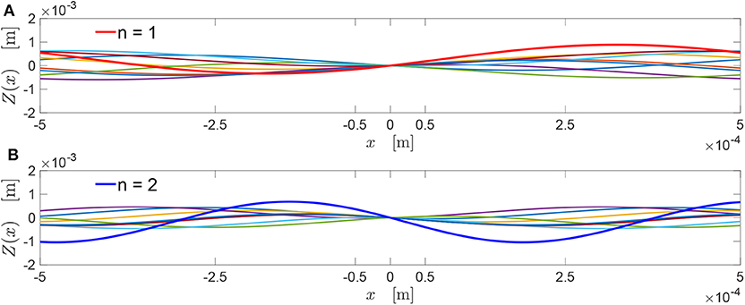
Figure 1. (A) The chromosome ${{C}}_1(x)$ is visualized by the red line, and corresponds to the sum of the other colored co-sinusoids with n = 1. (B) The chromosome ${{C}}_2(x)$ corresponds to the set of co-sinusoids provided by the choice n = 2.

The chromosome ${{C}}_1(x)$ is assumed to have a wavelength equal to the sample wavelength, i.e., λ₁ = L = 100 μm. This chromosome, depicted by a thick red line in Figure 1A, is obtained by summing all the ${M}=8$ co-sinusoids with the associated value n = 1.

The chromosome ${{C}}_2(x)$, depicted by blue line in Figure 1B, is obtained as the sum of all the ${M}=8$ co-sinusoids with n = 2. Then, since it is imposed γ = 1.5, the chromosome ${{C}}_2(x)$ has ${\lambda }_2=\frac{{\lambda }_1}{1.5}=\text{66.6}\mu \text{m}$.

Each of the two chromosomes in Figure 1 maintains a co-sinusoidal shape with the same wavelength λ_n as the associated parent co-sinusoids, and with a phase angle θ. Its height field in Equation (2) can be also written as

$\begin{array}{ll}{{C}}_n(x)={{G}}_n\left\{g_{n,1}\left[1-cos\left(\frac{2\pi }{\lambda }{\gamma }^{n-1}x\right)\right]+g_{n,2}sin\left(\frac{2\pi }{\lambda }{\gamma }^{n-1}x\right)\right\}.& (5)\end{array}$

In Equation (5), the amplitude parameter ${{G}}_n={A}\sqrt{\frac{{log}_{10}(\gamma )}{{M}}}{\left(\frac{2\pi }{\lambda }\right)}^{-{H}}{\gamma }^{-(n-1){H}}$ has been introduced, together with the two constants g_n,1 and g_n,2, which depend on the phases ϕ_m,n of the ridges with first index m:

$\begin{array}{ll}{g}_{n,1}={\displaystyle \sum _{m=1}^{{M}}}cos({\varphi }_{m,n}),g_{n,2}={\displaystyle \sum _{m=1}^{{M}}}sin({\varphi }_{m,n}).& (6)\end{array}$

A feasible mathematical model of a chromosome might be one in a form similar to that of the MWM function in Equation (1) with ${M}=1$ and a single value of n, obtained by introducing the parameters ${{K}}_n$, θ_n,1, and θ_n,2:

$\begin{array}{ll}{{C}}_n(x)={{K}}_n\left[cos({\theta }_{n,1})-cos\left(\frac{2\pi }{\lambda }{\gamma }^{n-1}x+{\theta }_{n,2}\right)\right].& (7)\end{array}$

A particular case of Equation (7) is when the angles θ_n,1 and θ_n,2 coincide, say, with the same θ_n. In such a case, a chromosome is described exactly according to the MWM profile in Equation (1) with ${M}=1$ and a single value of n. The expressions of ${{K}}_n,{\theta }_n$ in Equation (7) are obtained equating Equations (5) and (7), and are given by

$\begin{array}{ll}\{\begin{array}{l}{{K}}_n={{G}}_n\sqrt{{M}+2g_{n,3}},\\ {\theta }_n=arccos\left(\frac{g_{n,1}}{\sqrt{{M}+2g_{n,3}}}\right),\end{array}& (8)\end{array}$

where the parameter g_n,3 is defined as follows:

$\begin{array}{ll}{g}_{n,3}={\displaystyle \sum _{i=1}^{{M}-1}}{\displaystyle \sum _{j=i+1}^{{M}}}cos({\varphi }_{j,n}-{\varphi }_{i,n}).& (9)\end{array}$

For its validity, Equation (8) requires the argument of $arccos\left(\frac{g_{n,1}}{\sqrt{{M}+2g_{n,3}}}\right)$ to be between −1 and 1, i.e.,

$\begin{array}{ll}\left|g_{n,1}\right|\le \left|\sqrt{{M}+2g_{n,3}}\right|.& (10)\end{array}$

In the above, the additional condition ${M}+2g_{n,3}\ge 0$ has not been imposed explicitly, since it always holds. Indeed, one can easily check that ${M}+2g_{n,3}$ is the square of the Euclidean norm of the vector with components (${\displaystyle \sum _{i=1}^{{M}}}cos({\varphi }_{i,n}),{\displaystyle \sum _{i=1}^{{M}}}sin({\varphi }_{i,n})$). Of course, this norm is always larger than or equal to 0.

A numerical simulation has been conducted to verify the validity of condition (10). This has been evaluated for several values of ${M}$, considering each time 1,000 random choices (uniformly and independently sampled between 0 and 2π) for the phases. Figure 2 reports, for each such value of ${M}$, the percentage of cases for which Equation (10) is satisfied. Such percentage ranges between 88.5 and 98%, with an average value of ~95%.

FIGURE 2

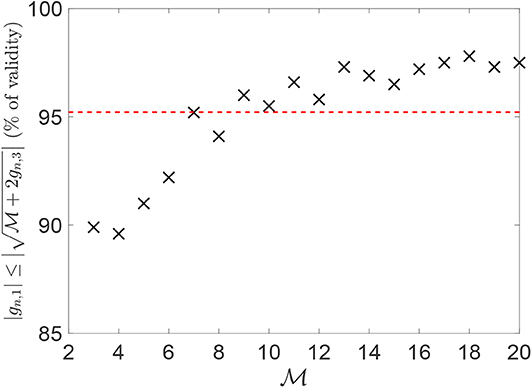
Figure 2. Percentage of validity of Equation (10) over 1,000 random choices for the phases (uniformly and independently sampled between 0 and 2π), for each value of ${M}$. The red line depicts the average percentage of validity.

2.3. Roughness Reconstruction Over Multiple Length Scales

The definition of chromosome allows the reconstruction of profiles Z(x) over multiple approximate realizations of the same surface. This can be done by limiting the summation in Equation (3) to a subset of chromosomes ${{C}}_n(x)$.

For both the stiffness-load curve K(p) and the area-load curve A(p), only one subset of the chromosomes can be considered to represent the main features of the contact mechanics response. This is shown in Figure 3 for a representative example coming from a fractured alloy interface (black line), considering both the K(p) and A(p) evolutions. The red dashed line is the contact mechanics response of the profile obtained by summing up chromosomes that have a K(p) evolution with a correlation coefficient larger than 0.95 with the complete K(p) one. Both the K(p) and A(p) evolutions of this profile overlap significantly with the ones corresponding to the complete profile, which is obtained when all the chromosomes are taken into account in the summation. This means that the interaction of chromosomes composing only one part of the complete genome is sufficient to approximate the stiffness-load curve K(p) well, as previously deduced in Paggi and Barber (2011).

FIGURE 3

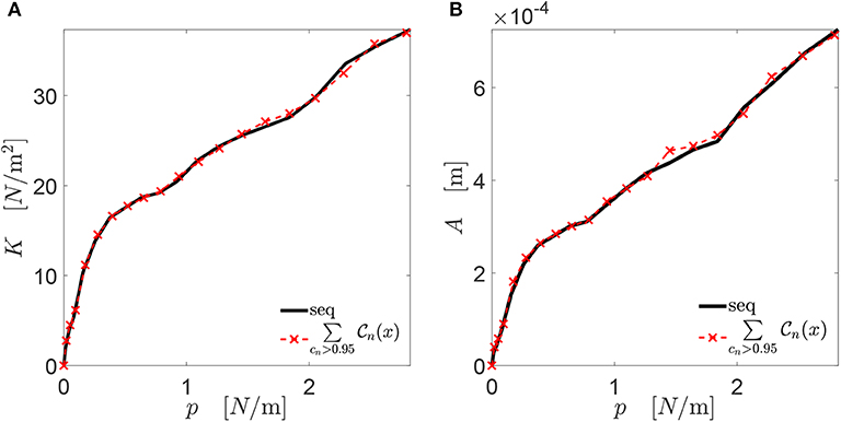
Figure 3. Mechanical curve K(p) in (A) and A(p) in (B) for the alloy fractured profile in the one-dimensional case. The red line refers to the contact mechanics response of the profile obtained summing up all the chromosomes with a correlation coefficient c_n larger than 0.95 with the complete K(p) curve. In the legend, “seq” stands for “sequenced,” and refers to the complete profile (the one identified from the whole set of genes).

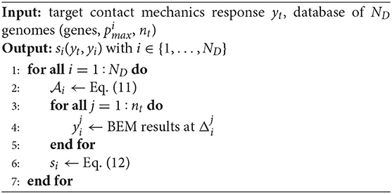
The selection of chromosomes outlined above is detailed in Algorithm 1. From the genome of a surface, one obtains the K(p) evolution of the profile described by Equation (1) (Step 1). The mechanical curves K_n(p) of all the n_c chromosomes composing the considered rough profile are iteratively extracted using the BEM algorithm for the frictionless elastic normal contact problem, which is solved via the Non-Negative Least Squares method proposed in Bemporad and Paggi (2015) (Steps 2–7). The correlation coefficients c_n between the extracted curves and the one K(p) of the complete rough profile are calculated (see Step 6). Only chromosomes with a correlation coefficient higher than 0.95 are then retained in the final set U_c of chromosomes (see Step 8).

ALGORITHM 1

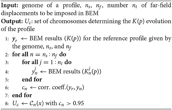
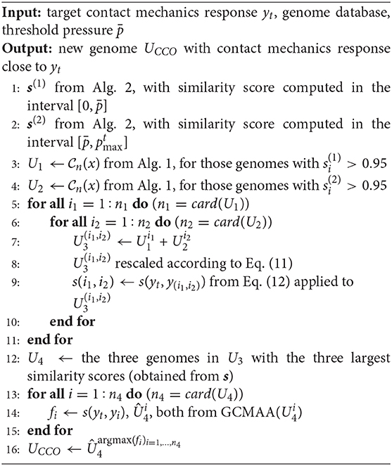
Algorithm 1. Chromosome selection

3. Genetic Algorithms to Identify Optimal Profiles to Match Target Contact Mechanics Responses

The goal of this section is to illustrate methods aimed to design a prototype profile able to achieve a target contact mechanics response y_t(ξ) of a rough profile, where t stands for “target”. This contact mechanics response depends on the specific needs of the frictionless elastic normal contact problem and is discretized using n_t points, where n_t is the number of far-field displacements Δ imposed to the frictionless elastic normal contact problem (see Johnson, 2003; Bemporad and Paggi, 2015). This target evolution y_t(ξ) can be, e.g., either the stiffness-load curve K(p) or the contact area-displacement curve A(Δ). The unknown rough profile Z_t(x) to be identified is discretized using N = 512 nodes for a length L. Then, the values of n_s and n_f are defined according to Equation (4). Here, without loss of generality and for simplicity, it is imposed n_s = 1 for each realization. The frictionless elastic normal contact problem is solved in n_t = 20 equi-spaced rigid body displacements from the topmost summit of the considered profile to its deepest valley.

In the following, the variable ξ is taken as the contact pressure p. Moreover, the gene ${{A}}_i$ of a generic genome (indexed by i in the database) is rescaled to match a given pressure requirement, $p\le p_{max}^t$, as follows:

$\begin{array}{ll}{{A}}_i\leftarrow \frac{p_{max}^t}{p_{max}^i}{{A}}_i.& (11)\end{array}$

The maximum pressure $p_{max}^i$ is computed imposing a far-field displacement equal to the original profile amplitude. In such a way, the new profile shows a maximum pressure $p_{max}^t$ if a far-field displacement equal to the peak-valley amplitude is considered to solve the frictionless elastic normal contact problem.

Three different methods to design the prototype profile are proposed. All these methods start from a known database of genomes. In the first case, a genome is selected that has the closest contact mechanics response to y_t among all the genomes in the database. Its genes are then optimized to increase the similarity with the target contact mechanics response. In the second case, two genomes are selected that match the target response in different imposed ranges Δp. Then, these genomes are combined using an optimized cross-over mechanism. The third and last case is similar to the second one but, instead of the complete genomes, two sets of chromosomes are mixed. These two sets are contained in two genomes that match the target response in different imposed ranges Δp.

3.1. Simple Optimization of Genes

In this section, the Simple Optimization of Genes (SOG) genetic algorithm is presented. Genes to be optimized belong to a genome producing a rough profile with a contact mechanics response very similar to the target one. The following similarity score

$\begin{array}{ll}{s}_i=s(y_t,y_i)=1-{\Vert \frac{y_t(\xi )-y_i(\xi )}{y_t(\xi )}\Vert }_{\infty }& (12)\end{array}$

is defined to quantify how much the target contact mechanics response, y_t(ξ), and the one y_i(ξ) associated with the parent i-th rough profile, are similar. Here, ‖·‖_∞ denotes the l_∞-norm, computed on the n_t points used to discretize the contact mechanics response. Due to Equation (12), the i-th curve coincides with the target one when s_i = 1 holds. Otherwise, it is close to the target one when s_i ≃ 1 holds.

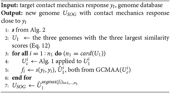
The numerical steps performed to select the best profile from the set of N_D genomes in the given database are described in Algorithm 2. The similarity score in Equation (12) is computed for all the N_D rough profiles available in the database, rescaled according to Equation (11) (Step 2). The contact mechanics response y_i(ξ) is computed via BEM, considering n_t different far-field displacements, from 0 to the new profile amplitude (Steps 3–5). Finally, s_i = s(y_t, y_i) in Equation (12) is computed (Step 6).

ALGORITHM 2

Algorithm 2. Similarity score extraction from a database of genomes

Genes belonging to the three genomes with the three largest associated values of s(y_t, y_i) are now optimized using the Globally Convergent Method of Moving Asymptotes (GCMMA) (Svanberg, 2002). This is an iterative optimization algorithm, which is often used in optimal design for mechanical problems (see Bacigalupo et al., 2016, 2017 for some of its recent applications to band gap optimization). The GCMMA algorithm replaces a nonlinearly constrained optimization problem by a sequence of approximating nonlinearly constrained optimization subproblems, which are simpler to solve. In the work, the objective function has been chosen to be the square of the similarity score, i.e., $s^2(y_t,y_i)$, in order to increase its smoothness. The GCMMA iterative solution is obtained after a number n_it of steps, starting from an initial choice for the vector of optimization variables. In the case of the SOG, this initial choice is provided by Algorithm 2, which provides an initial value of the similarity score close to 1. In such a way, there is no risk to get a negative similarity score by locally maximizing its square.

To save CPU time, the number of variables in the optimization problem is limited as follows. The genes ${H}$, λ, and γ determine the frequency spectrum, i.e., the interaction among different length scales. Therefore, they are not varied during the optimization, but fixed to their original values. The gene ${A}$ is varied at each optimization step to satisfy the pressure requirement, according to Equation (11). So, only the phases ϕ_m,n are considered as optimization variables. In the optimization, their values are constrained in the range between ∓10% of their initial values, to preserve the main features of the original chromosomes. Moreover, only the phase genes ϕ_m,n of chromosomes that determine the main features of the K(p) response are considered. Such genes are selected according to Algorithm 1.

Finally, the SOG algorithm is summarized in Algorithm 3. Starting with a profile scouting from the available database (Step 1), the three profiles whose contact mechanics responses are most similar to the target y_t are chosen (Step 2). The genes of each such genome are then optimized using the GCMMA algorithm (Steps 3–6), limiting the optimization variables only to the chromosomes determining the main features of the target y_t, as determined by Algorithm 2. The resulting optimized genomes are denoted by ${Û}_1^i$. Finally, among such genomes, the new genome is chosen as the one with the best (square of the) similarity score with respect to the target response (Step 7). In this last step, argmax(f_i)_{i = 1, …, n1} denotes the index i associated with the largest f_i.

ALGORITHM 3

Algorithm 3. Simple Optimization of Genes (SOG)

3.2. Genome Cross-Over

In this section, the Genome Cross-Over (GCO) genetic algorithm is presented. In this method, different pairs of genomes are mixed, to obtain a new genome matching the target response y_t(ξ). The best pair of genomes is chosen in relation to their similarity scores in two specific ranges of the target response y_t(ξ).

This concept is explained through Figure 4, where a target response y_t(p) is shown by the red line. For the sake of explanation, two curves y₁(p) (dashed black line) and y₂(p) (dashed dot blue line) have been manually generated, which have a similarity score with respect to y_t(p) equal to s₁ ≃ 0.89 and s₂ ≃ 0.88, respectively.

FIGURE 4

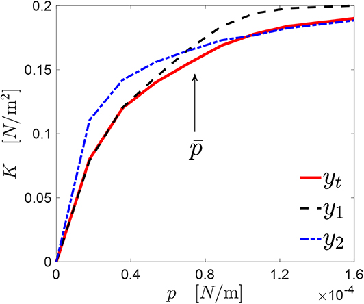
Figure 4. A generic profile y₁(p) approximates the target response y_t(p) [here, K(p)] accurately under a certain level of pressure $\bar{p}$. At the opposite, another profile y₂(p) provides a good approximation of y_t(p) only above $\bar{p}$.

However, the curves y₁(p) and y₂(p) describe quite accurately the curve y_t(p) in different ranges of pressures, if a suitable threshold pressure $\bar{p}$ is defined. The value of $\bar{p}$ can be chosen arbitrarily, or might be imposed by the particular problem formulation. In the specific case shown in the figure, in the interval $\left[0,\bar{p}\right]$, the curve y₁ represents with good accuracy y_t [s₁(y_t, y₁) ≃ 0.97]. The same happens in the interval $\left[\bar{p},p_{\text{max}}^t\right]$ for the curve y₂ [s₂(y_t, y₁) ≃ 0.99].

Then, it is reasonable to expect that a new profile obtained by combining the two genomes associated with y₁ and y₂, respectively, should provide a contact mechanics response closer to y_t over the whole range of pressures. However, mixing these two genomes may also lead to a very different roughness organization. For this reason, the GCO iterative scheme checks if the new genome, obtained by mixing the genome of y₁ and the one of y₂, is able to represent accurately y_t over the whole range of pressures, before using the GCMMA algorithm to increase the value of the similarity score.

The GCO structure is presented in Algorithm 4. According to the value of $\bar{p}$, two different sets U₁ and U₂ are identified from the database of genomes (Steps 1–2). The first set U₁ contains the genomes with a value of the similarity score (Equation 12) larger than 0.95 in the interval $\left[0,\bar{p}\right]$ (Step 3). The second set U₂ contains the genomes with a value of the similarity score (Equation 12) larger than 0.95 in the interval $\left[\bar{p},p_{\text{max}}^t\right]$ (Step 4). All possible combinations of genomes from the two sets above are now considered, defining the set U₃ (Step 5–11). A new genome corresponds to each of these combinations, whose gene ${A}$ is rescaled according to Equation (11) (Step 8). Then, the value of the similarity score (Equation 12) is computed with respect to the target response (Step 9). The three new genomes showing the three largest values of the similarity score are used as inputs to the GCMMA algorithm, defining the set U₄ (Step 12). Also in this case, the number of genes to be optimized is limited, considering only the phases ϕ_m,n associated with the chromosomes that determine the main features of the K(p) evolution of the parent curve (see Algorithm 1). The new genome U_GCO with the maximum value of the similarity is finally identified (Step 17).

3.3. Chromosomes Cross-Over

ALGORITHM 4

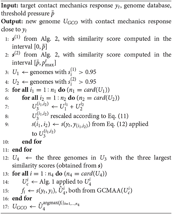
Algorithm 4. Genome Cross-Over (GCO)

In this section, the Chromosomes Cross-Over (CCO) genetic algorithm is presented. We recall that, as observed in section 2, the main features of the contact mechanics response of a rough profile are determined by specific chromosomes of the genomes. This subdivision allows the introduction of a chromosomes selection step to reduce the number of variables to be optimized using the GCMMA algorithm, as presented before for the SOG (section 3.1) and the GCO (section 3.2).

In the CCO method, only chromosomes determining the main features of the contact mechanics responses of two different genomes are mixed to match the target response y_t. These two sets of chromosomes come from genomes that have the largest values of the similarity score in specific ranges of the target response y_t, as done for the GCO method (see section 3.2). Then, in this case the GCMMA is applied to the complete set of chromosomes composing this new genomes, since they all determine its mechanical evolution.

The CCO iterative scheme is summarized in Algorithm 5. According to the value of the threshold pressure $\bar{p}$, two different sets U₁ and U₂ of reduced genomes are identified, starting from the given database (Steps 1–2). The first set U₁ is obtained as follows. First, one generates a subset of genomes that show a value of the similarity score (Equation 12) larger than 0.95 in the interval $\left[0,\bar{p}\right]$ (Step 3). Then, these genomes are reduced, limiting to those chromosomes that affect the K(p) evolution significantly. Such chromosomes are selected according to Algorithm 1. The resulting reduced genomes form the set U₁. The second set U₂ is obtained in a similar way as U₁, but computing the similarity score in the interval $\left[\bar{p},p_{\text{max}}^t\right]$ (Step 4). All possible combinations of these reduced genomes from the two sets above are now considered, defining the set U₃ (Steps 5–11). A new genome corresponds to each of these combinations. Its amplitude gene ${A}$ is rescaled according to Equation (11), to match the pressure requirement (Step 8). Then, the value of the similarity score (Equation 12) is computed with respect to the target response (Step 9). The three new genomes showing the three largest values of the similarity score are used as inputs to the GCMMA algorithm, defining the set U₄ (Step 12). Only in the case of the CCO algorithm, the GCMMA algorithm is applied to all the genes of this new genome, as the size of the optimization problem has been already reduced in Steps 3–4. The new genome U_CCO with the maximum obtained value of the similarity score is finally identified (Step 16).

ALGORITHM 5

Algorithm 5. Chromosomes Cross-Over (CCO)

4. Optimal Genome to Match a Specified Contact Mechanics Response

In this section, the genetic algorithms described in section 3 are compared in their application to a representative example. Before doing that, the characteristics of the numerical genome database considered in the paper are reported. Then, the set-up of the numerical experiment proposed is introduced. Finally, the related results are discussed, focusing the attention on the characterization of the so-obtained new genomes.

4.1. Database of Genomes

A database of genomes is needed to apply all the genetic algorithms proposed in the paper. In the following, a small database is generated numerically, to show a representative example of this approach. To generate the database, the amplitude parameter is fixed to ${A}=1$, and the main wavelength is put equal to λ = 849.42 μm.

The number of ridges is set to ${M}=1$, to save computational time. This particular case corresponds to chromosomes described according to Equation (7) with θ_n,1 = θ_n,2 = θ_n. As discussed in section 2, this can be considered as representative of several situations for a rough profile. Each profile Z_i(x) is then discretized using N = 512 nodes. The elastic modulus is imposed to be equal to E = 1 MPa. Furthermore, n_h = 20 different pairs of values for ${H}$ and γ are considered. They are generated according to a Sobol' sequence (Niederreiter, 1992) (see Figure 5A), with ${H}$ ranging between 0.5 and 1.5, and γ between 1.4 and 2. The value of γ is chosen in such a way to keep small the number of frequencies composing the profile spectrum (see Equation 4), thus limiting the computational costs. Also the phase matrix Φ is generated according to a Sobol' sequence. This matrix is made of n_ϕ = 5 columns, corresponding to 5 choices for the set of phases. The number of rows is equal to the maximum possible number of phases for these choices of the parameters. According to Equation (4), such number is obtained in correspondence of the smallest value of γ. Then, N_D = n_hn_ϕ rough profiles Z_i(x) are generated, combining each pair (${H}$, γ) to each column of Φ, considering only the number of values needed for the phases.

FIGURE 5

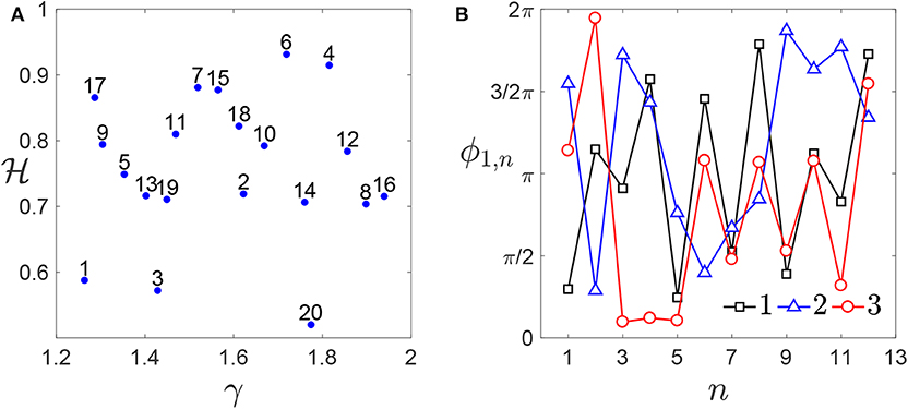
Figure 5. Genome database: (A) enumeration of all the pairs ${H}$ and γ generated. (B) First thirteen elements of the first three columns of the matrix Φ (${M}=1$), which are common to each combination. A larger number of phases is considered for smaller values of γ (i.e., for γ < 1.6).

4.2. Set-Up of the Numerical Experiment

In Figure 6, the contact mechanics response y_t = K(p) is depicted through the black line. All the values are considered independent from E, as this is equal to unity. Also the K(p) responses of all the genomes in the generated database are visualized in Figure 6. The target contact mechanics response y_t has been generated manually, and has a trend similar to the ones belonging to the database. The maximum pressure reachable is imposed to be $p_{max}^t=1.6\times 10^{-4}\text{N}/\text{m}$. This value is larger than the ones of all the genomes in the database considering, for each profile, a far-field displacement equal to the profile amplitude.

FIGURE 6

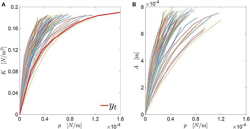
Figure 6. (A) Target curve y_t = K(p) along with all the corresponding curves associated with the genomes in the generated database; (B) all A(p) curves associated with those genomes.

For each algorithm, the stage just preceding the application of the GCMMA algorithm is referred to as “GCMMA (0).” For the SOG, it corresponds to the selection of the three best values obtained from the scouting of the database (Step 2 in Algorithm 3). For both the GCO and the CCO algorithms, it corresponds to the computation of the similarity scores of the new genomes determined after the cross-over (Step 12 in both Algorithms 4 and 5). For the SOG, the GCMMA algorithm is applied with n_it = 5, while for the GCO and CCO, only with n_it = 3. The output of this optimization step is denoted by “GCMMA (1).” These different choices for n_it are made in order to have comparable computational times of about 1 minute. In such a way, it is possible to observe variations in the results in a sufficiently small time, enabling in-line control as a possible successive step. Moreover, in the numerical experiment, for the SOG and GCO algorithms, the GCMMA is also applied in a second optimization step, whose output is denoted as “GCMMA (2),” using n_it = 2 iterations. In this case, the genes to be optimized are the ones referred to the chromosomes excluded in the selection step (see Algorithm 1). For the CCO, this second step cannot be applied since these chromosomes are excluded in the first part of the algorithm (Steps 1–4 in Algorithm 5). However, to make the notation uniform for the three algorithms, a fictitious “GCMMA (2)” output is introduced for the CCO, by duplicating the results of “GCMMA (1).”

4.3. Numerical Results

The values of the similarity score s given by Equation (12) for the genomes obtained by combination and optimization using the SOG, GCO, and CCO algorithms are reported in Figure 7. The threshold pressure used for both the GCO and CCO is set equal to $\bar{p}=0.08$ [1/mm]. For each algorithm, solutions at different stages are reported in the figure. The first ones correspond to the three best solutions obtained in the first stage of each algorithm, before the application of the GCMMA (such solutions are represented in the figure by the triangle, circle, and cross, in increasing order). The figure shows that all the algorithms are quite efficient in matching the target contact mechanics response, achieving large values for the similarity score. The application of the GCMMA is beneficial for all the algorithms. However, the GCO and CCO algorithms might provide even better solutions by varying the threshold pressure $\bar{p}$.

FIGURE 7

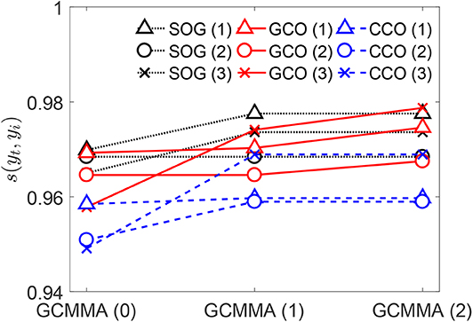
Figure 7. For the outputs of the SOG, GCO, and CCO algorithms, values of the similarity scores with respect to the target curve y_t. The threshold pressure is $\bar{p}=0.08$ for both the GCO and CCO.

4.4. Effect of the Threshold Pressure $\bar{p}$

A threshold pressure $\bar{p}$ has been introduced for the GCO and the CCO, to select individual genomes able to approximate locally the target curve with a good accuracy. Additional simulations have been made, to assess the sensitivity of the results with respect to such a parameter. Both the GCO and CCO algorithms have been applied with different values of $\bar{p}$. Such values have been chosen between 0.5 × 10⁻⁴N/m and 1.1 × 10⁻⁴N/m. A significant variation on the maximum value of the similarity score is observed for the GCO algorithm (see Figure 8A). On the contrary, the CCO algorithm seems to be not affected by the value of $\bar{p}$, and the new genomes obtained by that algorithm are composed by the same starting genomes, independently of the threshold pressure $\bar{p}$. This may be due to the fact that our investigation has been conducted starting from a small database of genomes. In Figure 8B, the cardinality of the set U₃ is presented, for both the GCO and CCO algorithms. This set contains the new genomes obtained after the cross-over of genomes/chromosomes. The white part indicates, for both algorithms, the number of genomes whose value of the similarity score with respect to the target curve y_t is larger than 0.95. The cardinality of the set U₃ varies significantly with $\bar{p}$, and is the same for both algorithms. Nevertheless, the GCO algorithm is more efficient in terms of the obtained similarity with the target curve.

FIGURE 8

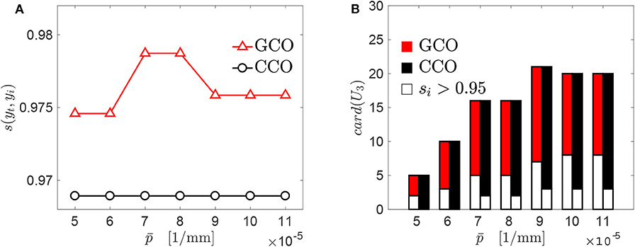
Figure 8. Sensitivity of the GCO and CCO outputs with respect to $\bar{p}$: (A) best similarity scores obtained for each algorithm. (B) Cardinality of the set U₃ which contains the new genomes obtained just before the application of the GCMMA, i.e., at the stage “GCMMA (0)” in Figure 7.

4.5. Description of the Optimized Genomes Representing y_t

The best three new genomes obtained at the end of the three algorithms presented in this paper have contact mechanics responses overlapping significantly with the target curve (see Figure 9A). However, the three genomes present different evolutions of the bearing area, as depicted in Figure 9B. Only the A(p) curves obtained by the SOG and GCO are similar. This may be due to the fact that, in the case of the CCO, high-frequency features of the rough profile might have been neglected. This is clear from Figures 10, 11.

FIGURE 9

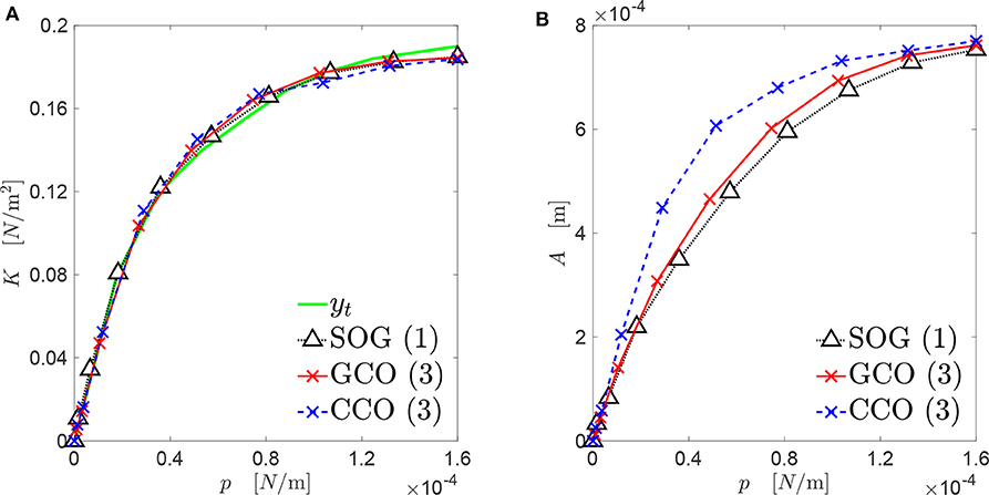
Figure 9. Mechanical behavior of the best rough profiles (see Figure 10), that approximate the target curve y_t: (A) contact stiffness versus contact pressure; (B) real contact area versus contact pressure.

FIGURE 10

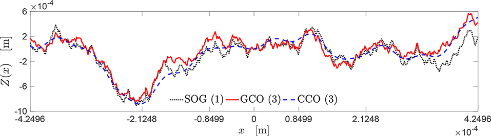
Figure 10. Topography of the best rough profiles approximating the target curve y_t (see Figure 9).

FIGURE 11

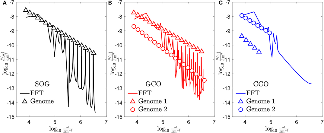
Figure 11. Power spectral density of the obtained new genomes, whose associated profiles are shown in Figure 10: (A) case of the SOG algorithm; (B) case of the GCO algorithm; (C) case of the CCO algorithm.

The topography of these rough profiles is presented in Figure 10. The profiles obtained by the SOG, GCO, and CCO algorithms are depicted, respectively, through a black dash dot-line, a red dashed line, and a blue continuous line. All these profiles have very similar geometrical features, regarding the locations of peaks and valleys. Moreover, it is interesting to notice that the profile provided by the CCO algorithm is a good approximation of the profile given by the GCO algorithm, which presents more high-frequency features.

To conclude, the discrete Power Spectral Density (PSD) P(ω) of the new obtained genomes is shown in Figure 11, and is represented by markers in both sub-figures. For each case, the continuous PSD function, which is obtained through the Fast Fourier Transform (FFT) filtering (Berry and Lewis, 1980), is shown by a continuous line. For the SOG (see Figure 11A), the peaks of the continuous PSD function match the discrete one accurately for high frequencies. No good matching is found for low frequencies. The same remark holds for the case of the GCO (see Figure 11B). Here, the spectrum is more dense and, only for high frequencies, peaks of the continuous PSD function are located in the same positions of the genome. For both the SOG and the GCO, a consistent difference in the amplitude of P(ω) is found. Finally, the spectrum of the profile obtained by the CCO is composed by a small set of frequencies. The high-frequency part of the PSD is flat. In this case, the discrete power spectral density is nearly proportional to the one of the SOG in the low-frequency range. Since the GCO approximation of the target curve is obtained using a smaller set of chromosomes, it can be easily controlled for the case of in-line control of the rough profile morphology. However, in this case, the PSD is almost flat, and some peaks are found in frequencies where there are no genome components.

5. Conclusion

The main goal of this work was to provide a mathematical and computational methodology to identify new surface topologies with given target contact mechanics responses, based on a multi-scale characterization of roughness. This was described by a superposition of a finite set of successive length scales of roughness, where each scale is associated with a particular form of the MWM function, named chromosome. Based on this representation, three genetic algorithms were proposed to combine profiles and identify the best one which meets the given target contact mechanics response.

The first genetic algorithm (Simple Optimization of Genes, SOG) optimizes the genes of a known genome. Embedded in the SOG, an iterative optimization algorithm (the GCMMA) was used to increase the similarity with the target contact mechanics response. To save computational time, optimization was performed only with respect to the dominant chromosomes of the genome, i.e., the ones for which the correlation coefficient between the associated contact mechanics response and the target one is above a given threshold.

The second genetic algorithm (Genome Cross-Over, GCO) crosses-over two different genomes that show a high similarity with respect to the target response in two given intervals determined by a threshold pressure $\bar{p}$. Also in this case, only dominant chromosomes were optimized to save computation time.

The third genetic algorithm (Chromosomes Cross-Over, CCO) consists in a cross-over of chromosomes that provide the main features of the contact mechanics responses of two genomes that well approximate the target curve in two reference intervals determined by the threshold pressure $\bar{p}$. In this case, GCMMA was applied to the complete new genome, since the number of optimization variables is smaller than for the other two approaches.

The three genetic algorithms proposed in this work generated profiles that almost fully reproduce the given K(p) curve, when this is chosen as the target contact mechanics response. Also, they have in common similar features regarding their topography, such as the locations of peaks and valleys. This characterization might be caused by the fact that a limited number of genomes was present in the database used for the numerical experiment reported in the paper. A much wider set of profile topologies is expected to be obtained by exploiting a significantly larger database, facilitating the discovery of optimal patterns/textures, based on the specific needs. Also, the investigation can be extended to all the genomes that provide a good approximation of the target curve, in order to identify some geometrical features that drive the elastic response of a rough profile. Once identified, these features can be taken into account in the optimization by adding specific chromosomes, to be controlled in the case of in-line profile morphing.

Finally, the authors would like to remark that the proposed approaches could be extended to the two-dimensional case, although this is expected to require a larger computational effort. Moreover, the use of micromechanical contact theories such as those compared in Zavarise et al. (2007) and Paggi and Ciavarella (2010) could be another interesting research direction. For instance, one could assume not to have the surface height field at all, but only a set of relevant statistical parameter inputs of micromechanical contact theories. In such a context, the search for the optimal topology to match a prescribed contact response would reduce to the identification of the statistical parameters based on the combination of the initial dataset and of the proposed genetic algorithms.

Data Availability Statement

The dataset generated for this study is available on request to paolo.cinat@alumni.imtlucca.it.

Author Contributions

All authors listed have made a substantial, direct and intellectual contribution to the work, and approved it for publication.

Funding

MP acknowledges the support of MIUR-DAAD to the Joint Mobility Program 2017 Multi-Scale Modeling of Friction for Large Scale Engineering Problems.

Conflict of Interest

The authors declare that the research was conducted in the absence of any commercial or financial relationships that could be construed as a potential conflict of interest.

References

Ausloos, M., and Berman, D. (1985). A multivariate Weierstrass-Mandelbrot function. Proc. R. Soc. Lond. A 400, 331–350. doi: 10.1098/rspa.1985.0083

CrossRef Full Text | Google Scholar

Bacigalupo, A., Gnecco, G., Lepidi, M., and Gambarotta, L. (2017). Optimal design of low-frequency band gaps in anti-tetrachiral lattice meta-materials. Compos. Part B Eng. 12, 341–359. doi: 10.1016/j.compositesb.2016.09.062

CrossRef Full Text | Google Scholar

Bacigalupo, A., Lepidi, M., Gnecco, G., and Gambarotta, L. (2016). Optimal design of auxetic hexachiral metamaterials with local resonators. Smart Mater. Struct. 25:054009. doi: 10.1088/0964-1726/25/5/054009

CrossRef Full Text | Google Scholar

Barber, J. (2003). Bounds on the electrical resistance between contacting elastic rough bodies. Proc. R. Soc. Lond. A 459, 53–66. doi: 10.1098/rspa.2002.1038

CrossRef Full Text | Google Scholar

Bemporad, A., and Paggi, M. (2015). Optimization algorithms for the solution of the frictionless normal contact between rough surfaces. Int. J. Solids Struct. 69–70, 94–105. doi: 10.1016/j.ijsolstr.2015.06.005

CrossRef Full Text | Google Scholar

Berry, M., and Lewis, Z. (1980). On the Weierstrass-Mandelbrot fractal function. Proc. R. Soc. Lond. 370, 459–484. doi: 10.1098/rspa.1980.0044

CrossRef Full Text | Google Scholar

Bora, C., Flater, E., Street, M., Redmond, J., Starr, M., Carpick, R., et al. (2005). Multiscale roughness and modeling of MEMS interfaces. Tribol. Lett. 19, 37–48. doi: 10.1007/s11249-005-4263-8

CrossRef Full Text | Google Scholar

Borri, C., and Paggi, M. (2015). Topological characterization of anti-reflective and hydrophobic rough surfaces: are random process theory and fractal modeling applicable? J. Phys. D Appl. Phys. 48:045301. doi: 10.1088/0022-3727/48/4/045301

CrossRef Full Text | Google Scholar

Brettel, M., Friederichsen, F., Keller, M., and Rosenberg, M. (2014). How virtualization, decentralization and network building change the manufacturing landscape: an Industry 4.0 perspective. Int. J. Mech. Aerospace Indus. Mechatron. Eng. 8, 37–44. Available online at: https://publications.waset.org/9997144/pdf

Google Scholar

Buscaglia, G., Ciuperca, I., and Jai, M. (2007). On the optimization of surface textures for lubricated contacts. J. Math. Anal. Appl. 335, 1309–1327. doi: 10.1016/j.jmaa.2007.02.051

CrossRef Full Text | Google Scholar

Carr, J., and Benzer, W. (1991). On the practice of estimating fractal dimension. Math. Geol. 23, 945–958. doi: 10.1007/BF02066734

CrossRef Full Text | Google Scholar

Ciavarella, M., Demelio, G., Barber, J., and Jang, Y. (2000). Linear elastic contact of the Weierstrass profile. Proc. R. Soc. Lond. A 456, 387–405. doi: 10.1098/rspa.2000.0522

CrossRef Full Text | Google Scholar

Ciavarella, M., Murolo, G., Demelio, G., and Barber, J. (2004). Elastic contact stifness and contact resistance for the Weierstrass profile. J. Mech. Phys. Solids 52, 1247–1265. doi: 10.1016/j.jmps.2003.12.002

CrossRef Full Text | Google Scholar

Cinat, P., Paggi, M., and Gnecco, G. (2019). Identification of roughness with optimal contact response with respect to real contact area and normal stiffness. Math. Probl. Eng. 2019:7051512. doi: 10.1155/2019/7051512

CrossRef Full Text | Google Scholar

Farina, I., Fabbrocino, F., Colangelo, F., Feo, L., and Fraternali, F. (2016). Surface roughness effects on the reinforcement of cement mortars through 3D printed metallic fibers. Compos. Part B Eng. 99, 305–311. doi: 10.1016/j.compositesb.2016.05.055

CrossRef Full Text | Google Scholar

Gao, H., Wang, X., Yao, H., Gorb, S., and Arzt, E. (2005). Mechanics of hierarchical adhesion structures of geckos. Mech. Mater. 37, 275–285. doi: 10.1016/j.mechmat.2004.03.008

CrossRef Full Text | Google Scholar

Gujrati, A., Khanal, S. R., Pastewka, L., and Jacobs, T. D. B. (2018). Combining TEM, AFM, and profilometry for quantitative topography characterization across all scales. ACS Appl. Mater. Interfaces 10, 29169–29178. doi: 10.1021/acsami.8b09899

PubMed Abstract | CrossRef Full Text | Google Scholar

Guo, Q., Zhu, P., Li, G., Wen, J., Wang, T., Lu, D. D., et al. (2017). Study on the effects of interfacial interaction on the rheological and thermal performance of silica nanoparticles reinforced epoxy nanocomposites. Compos. Part B Eng. 116, 388–397. doi: 10.1016/j.compositesb.2016.10.081

CrossRef Full Text | Google Scholar

Guo, S.-J., Yang, Q.-S., He, X. Q., and Liew, K. M. (2014). Modeling of interface cracking in copper-graphite composites by MD and CFE method. Compos. Part B Eng. 58, 586–592. doi: 10.1016/j.compositesb.2013.10.042

CrossRef Full Text | Google Scholar

Johnson, K. (2003). Contact Mechanics. Cambridge, UK: Cambridge University Press.

Google Scholar

King, R., Stansfield, W., and Mulligan, P. (2006). A Dictionary of Genetics, 7th Edn. Oxford: Oxford University Press. doi: 10.1093/acref/9780195307610.001.0001

CrossRef Full Text | Google Scholar

Ko, K., Jin, S., Lee, S. E., Lee, I., and Hong, J.-W. (2019). Bio-inspired bimaterial composites patterned using three-dimensional printing. Compos. Part B Eng. 165, 594–603. doi: 10.1016/j.compositesb.2019.02.008

CrossRef Full Text | Google Scholar

Kwon, D.-J., Kim, J.-H., Kim, Y.-J., Kim, J.-J., Park, S.-M., Kwon, I.-J., et al. (2019). Comparison of interfacial adhesion of hybrid materials of aluminum/carbon fiber reinforced epoxy composites with different surface roughness. Compos. Part B Eng. 170, 11–18. doi: 10.1016/j.compositesb.2019.04.022

CrossRef Full Text | Google Scholar

Mandelbrot, B. (1977). Fractals: Form, Chance, and Dimension. San Francisco, CA: W. H. Freeman.

Google Scholar

Moghri, M., Madic, M., Omidi, M., and Farahnakian, M. (2014). Surface roughness optimization of polyamide-6/nanoclay nanocomposites using artificial neural network: genetic algorithm approach. Sci. World J. 2014:485205. doi: 10.1155/2014/485205

PubMed Abstract | CrossRef Full Text | Google Scholar

Moroni, F., Palazzetti, R., Zucchelli, A., and Pirondi, A. (2013). A numerical investigation on the interlaminar strength of nanomodified composite interfaces. Compos. Part B Eng. 55, 635–641. doi: 10.1016/j.compositesb.2013.07.004

CrossRef Full Text | Google Scholar

Niederreiter, H. (1992). Random Number Generation and Quasi-Monte Carlo Methods. Philadelphia, PA: SIAM. doi: 10.1137/1.9781611970081

CrossRef Full Text | Google Scholar

Nosonovsky, M., and Bushan, B. (2008). Multiscale Dissipative Mechanisms and Hierarchical Surfaces: Friction, Superhydrophobicity, and Biomimetics. Hoboken, NJ: Springer. doi: 10.1007/978-3-540-78425-8

CrossRef Full Text | Google Scholar

Nouari, M., Xiao, M., Shen, X., Ma, Y., Yang, F., Gao, N., et al. (2018). Prediction of surface roughness and optimization of cutting parameters of stainless steel turning based on RSM. Math. Probl. Eng. 2018:9051084. doi: 10.1155/2018/9051084

CrossRef Full Text | Google Scholar

Paggi, M., and Barber, J. (2011). Contact conductance of rough surfaces composed of modified RMD patches. Int. J. Heat Mass Transf. 54, 4664–4672. doi: 10.1016/j.ijheatmasstransfer.2011.06.011

CrossRef Full Text | Google Scholar

Paggi, M., and Ciavarella, M. (2010). The coefficient of proportionality k between real contact area and load, with new asperity models. Int. J. Solids Struct. 56, 1020–1029. doi: 10.1016/j.wear.2009.12.038

CrossRef Full Text | Google Scholar

Paggi, M., and Hills, D. A. (2020). Modeling and Simulation of Tribological Problems in Technology, Vol. 593 of CISM Courses and Lectures. Cham: Springer. doi: 10.1007/978-3-030-20377-1

CrossRef Full Text | Google Scholar

Sherge, M., and Gorb, S. (2001). Biological Micro- and Nano- Tribology & Nature's Solutions. Berlin: Springer.

Google Scholar

Svanberg, K. (2002). A class of globally convergent optimization methods based on conservative convex separable approximations. SIAM J. Optim. 12, 555–573. doi: 10.1137/S1052623499362822

CrossRef Full Text | Google Scholar

Vakis, A., Yastrebov, V., Scheibert, J., Nicola, L., Dini, D., Minfray, C., et al. (2018). Modeling and simulation in tribology across scales: an overview. Tribol. Int. 125, 169–199. doi: 10.1016/j.triboint.2018.02.005

CrossRef Full Text | Google Scholar

Wen, R., and Sinding-Larsen, R. (1997). Uncertainty in fractal dimension estimated from power spectra and variograms. Math. Geol. 29, 727–753. doi: 10.1007/BF02768900

CrossRef Full Text | Google Scholar

Wüst, P., Edelmann, A., and Hellmann, R. (2020). Areal surface roughness optimization of maraging steel parts produced by hybrid additive manufacturing. Materials 13, 1–17. doi: 10.3390/ma13020418

PubMed Abstract | CrossRef Full Text | Google Scholar

Xiaohan, Z., Xu, Y., and Jackson, R. (2017). An analysis of generated fractal and measured rough surfaces in regards to their multi-scale structure and fractal dimension. Tribol. Int. 105, 94–101. doi: 10.1016/j.triboint.2016.09.036

CrossRef Full Text | Google Scholar

Zain, A. M., Haron, H., and Sharif, S. (2008). “An overview of GA technique for surface roughness optimization in milling process,” in 2008 International Symposium on Information Technology, Vol. 4, 1–6. doi: 10.1109/ITSIM.2008.4631925

CrossRef Full Text | Google Scholar

Zavarise, G., Borri-Brunetto, M., and Paggi, M. (2007). On the resolution dependence of micromechanical contact models. Wear 262, 42–54. doi: 10.1016/j.wear.2006.03.044

CrossRef Full Text | Google Scholar

Zhang, J., Chen, J., and Kirby, E. (2007). Surface roughness optimization in an end-milling operation using the Taguchi design method. J. Mater. Process. Technol. 184, 233–239. doi: 10.1016/j.jmatprotec.2006.11.029

CrossRef Full Text | Google Scholar