Calculation of the BEM Integrals on a Variable Grid With the FFT

Introduction

The Boundary Element Method (BEM) is used in countless engineering disciplines. Among them is the field of Contact Mechanics where the approach has been applied with great success in recent years (Putignano et al., 2012; Müser et al., 2017; Popov et al., 2017; Li et al., 2018; Paggi and Hills, 2020). Another, yet much older example for a very successful application of the Boundary Element Method is the Aerodynamic Panel Method. Conceived by Hess and Smith at Douglas Aircraft in the early 1960s (for details, see Smith, 1990), the Aerodynamic Panel Method was among the first numerical implementations of the Boundary Element Method when electronic computers became available (for details, see Cheng and Cheng, 2005). Today, more than 60 years later, the method is still an essential tool in the aircraft industry for initial design studies (Anderson, 2017; Raymer, 2018). An example is the investigation of entirely new airplane designs, such as the Flying V (Benad, 2015; Faggiano et al., 2017; Palermo and Vos, 2020; Rubio Pascual and Vos, 2020). In the very first conceptual design stage of this project, panel methods were used to assess the aircrafts aerodynamics. While they describe only potential flow (for details, see Katz and Plotkin, 2001), the two main advantages of such methods are their ease of use and their computational speed. From a numerical perspective, only the boundary of the domain needs to be discretized which leads to simple meshing. When no measures are taken to accelerate the calculation, the computational complexity of a problem with N surface discretization points is O(N³) when direct solvers are used, and O(N²) using iterative solvers. While an O(N²) complexity is by current standards considered as expensive, it is still practical for initial design studies with a low number of surface panels. However, if a high number of discretization elements is required, or large parameter studies shall be conducted, one should consider accelerating the panel method. Several approaches exist for the reduction of the computational complexity of the Boundary Element Method (Phillips and White, 1997; Masters and Ye, 2004; Benedetti et al., 2008; Lim et al., 2008). An approach which has recently gained a lot of attention and has been very successful in the area of Contact Mechanics is to accelerate the calculation of the boundary integrals using the Fast Fourier Transformation (FFT) (Putignano et al., 2012; Pohrt and Li, 2014; Popov, 2017). It is natural perhaps, that this particular success should occur in the area of Contact Mechanics as one often considers a half-space surface in this field of research. A half-space surface aligns perfectly with a two-dimensional FFT-grid. Therefore, the calculation of the boundary integrals over the half-space can easily be performed with the FFT which reduces the computational complexity to O(NlogN^0.5). For arbitrary shapes however, this process is not as simple because the surface of an arbitrary shape does not align with a plane FFT-grid. In 1997, Philips and White developed a method for utilizing the Fast Fourier Transformation even for the calculation of boundary integrals on arbitrary shapes (Phillips, 1997). As it is illustrated in Benad (2018), the boundary integrals can be regarded as convolutions over a space which is one dimension higher than that of the boundary of an arbitrary shape. However, there are two main challenges when this realization is put into practice: First, even a three-dimensional regular FFT-grid which fully encloses the surface of an arbitrary shape never cuts through this surface precisely at its discretization points. Instead, the nodes of the regular grid lie either outside of the arbitrary shape, or inside the shape, but in general never directly on the surface, as it is the case for the half-space in the area of Contact Mechanics. Second, the computational complexity rises, when compared to the half-space. While the half-space fully aligns with a two-dimensional FFT-grid, an arbitrary shape requires a fully enclosing FFT-grid, that is, a three-dimensional convolution. This results in a complexity of O(N^1.5logN^0.75), which is lower than the O(N²) complexity of the standard boundary element procedure, but higher than the desired O(NlogN^0.5) complexity. Philips and White addressed both these issues in 1997 with their precorrected FFT method, which has often been referred to as pFFT. Therein, nearby panel interactions are calculated directly as in the standard boundary element procedure, and the far field is computed using the three-dimensional FFT-grid which fully encloses the surface. This FFT-grid may be much coarser than the surface mesh since higher order interpolation techniques are used to project the boundary values of the surface mesh points onto the nodes of the FFT-grid. This approach further reduces the O(N^1.5logN^0.75) complexity. At best, it is an O(NlogN) algorithm (Phillips and White, 1997).

It is remarkable how different the fields of application are, in which the pFFT approach can be used. When it was introduced by Philips and White, it was applied in the field of electrostatic analysis. But of course, the method can also be regarded as a more general FFT-based BEM in the area of Contact Mechanics which enables not only the calculation displacements and stresses of a half-space with the FFT, but of any arbitrary shape: (Masters and Ye, 2004) used the pFFT approach for the calculation of displacements and stresses in linear elastic solids of arbitrary shape with the Navier equation achieving O(NlogN) complexity. This makes the pFFT approach very appealing in the area of Contact Mechanics since the Boundary Element Method has proved to be a very robust tool in this area (Paggi and Hills, 2020), but is in its efficient practical application still somewhat restricted to the half-space. The pFFT may provide an opportunity to accelerate Boundary Element calculations of contact problems with a more difficult geometry. An exemplary application may be turbine blade fir-tree connections, a contact problem where the half-space theory is pushed to its limits (Benad, 2019). Naturally, the pFFT approach is not restricted to geometries where the domain of interest is the inner region which is enclosed by the boundary. Instead, it is also possible to consider the outer region. In 2006, Willis, Peraire and White utilized the pFFT to accelerate the Aerodynamic Panel Method achieving O(NlogN) complexity (Willis et al., 2006). The study investigated complicated shapes, and even unsteady applications with varying geometries such as flapping wings.

It seems that many fields of research may benefit from fast Boundary Element solvers. In the present study, an exemplary application of the pFFT will be shown for the 2D Navier equation. Using this example, it is illustrated how the pFFT might be extended to allow the application of the FFT with multiple discretization levels. This may lead to a further reduction in computational complexity to obtain the boundary integrals.

Governing Equation and Analytical Sample Solutions

Navier's equation is:

$\begin{array}{ll}\frac{1}{1-2\nu }{u}_{j,ji}+u_{i,jj}+\frac{1}{\mu }{b}_i=0& (1)\end{array}$

where i, j∈{1, 2, 3}, u_i are the displacements, ν is the Poisson's ratio, μ is the shear modulus, and b_i is the force density field (Hahn, 1985). Note that we choose to denote partial derivatives with $\frac{\partial }{\partial x_i}(\dots )={(\dots )}_{,i}$. For simplicity, we will in this work only consider the case of plane displacements where the Navier equation simply remains as in (1), but with i, j∈{1, 2} (Irgens, 2008). This case can be transformed to the case of plane stress by replacing ν with $\frac{\nu }{(1+\nu )}$ and leaving the value for μ unchanged (Irgens, 2008), see also (Galin, 2008) and (Kelly, 2013). Before we proceed, let us introduce analytical solutions for (1) which can later be used to validate the numerical results.

Uniformly Distributed Loads on Rectangular Body

A solution of (1) is

$\begin{array}{l}u=\frac{1-\nu }{2\mu }{\sigma }_{A}x-\frac{\nu }{2\mu }{\sigma }_{B}x+\frac{1}{2\mu }{\sigma }_{C}y,\\ v=\frac{1-\nu }{2\mu }{\sigma }_{B}y-\frac{\nu }{2\mu }{\sigma }_{A}y+\frac{1}{2\mu }{\sigma }_{C}x.& (2)\end{array}$

(Note that we choose to denote u_{i = 1} = u, u_{i = 2} = v, x_{i = 1} = x and x_{i = 2} = y.) For plane displacements, the corresponding stress field is simply:

$\begin{array}{ll}{\sigma }_{xx}={\sigma }_A,{\sigma }_{yy}={\sigma }_B,{\sigma }_{xy}={\sigma }_C,& (3)\end{array}$

which belongs, for example, to a rectangular body with uniformly distributed loads on the sides, see the left image in Figure 1. This simple problem, as well as arbitrarily shaped cut-outs (see the blue dashed line), can be used for validation purposes.

FIGURE 1

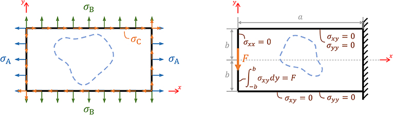
Figure 1. Left: A rectangular body with uniformly distributed loads. Right: A rectangular beam with an end load.

Bending of a Rectangular Beam by an End Load

We now turn to another exact solution of (1), which is often used to approximate the solution for a system as shown in the right image in Figure 1. A stress field for this problem with boundary conditions imposed for the stresses in the weak form reads (see Barber, 2004):

$\begin{array}{ll}{\sigma }_{xx}=\frac{3Fxy}{2b^3},{\sigma }_{yy}=0,{\sigma }_{xy}=\frac{3F(b^2-y^2)}{4b^3}.& (4)\end{array}$

With the material law of a linearly elastic isotropic solid (Gross et al., 2014), one obtains:

$\begin{array}{ll}{\epsilon }_{xx}=\frac{1-\nu }{2\mu }\frac{3Fxy}{2b^3},{\epsilon }_{yy}=-\frac{\nu }{2\mu }\frac{3Fxy}{2b^3},{\epsilon }_{xy}=\frac{1}{2\mu }\frac{3F(b^2-y^2)}{4b^3}& (5)\end{array}$

for the strains which belong to (4) for the case of plane displacements. Integration yields:

$\begin{array}{l}u=\frac{Fy}{8\mu b}\left(6+(1-\nu )\frac{3x^2}{b^2}+(\nu -2)\frac{y^2}{b^2}\right)-C_{1}y+C_3\\ v=\frac{Fx}{8\mu b}\left(-(1-\nu )\frac{x^2}{b^2}-\nu \frac{3y^2}{b^2}\right)+C_{1}x+C_2.& (6)\end{array}$

Setting u(x = a, y = 0) = 0 yields C₃ = 0. With u(x = a, y = b) = 0 one further obtains $C_1=\frac{F}{8\mu b}\left(4+(1-\nu )\frac{3a^2}{b^2}+\nu \right)$ and v(x = a, y = 0) = 0 yields $C_2=-\frac{Fa}{8\mu b}\left(4+(1-\nu )\frac{2a^2}{b^2}+\nu \right)$.

The result (6) for the displacements is an exact solution of (1) and may thus be used together with the corresponding stress field (4) as an analytical reference for comparison with the numerical results.

Note that at the boundary x = a the strains ε_yy in (5) are not zero as we would expect them to be for the beam which is displayed in the right image of Figure 1. Imposing the boundary conditions merely for the stresses in the weak form (see Barber, 2004) only gives an approximate solution for this set-up. The solution is fully accurate for a beam which is supported not by a solid wall, but a parabolic traction.

Boundary Integral Formulation

For the governing equation (1), Somigliana's identity (Gaul and Fiedler, 2013) relates the displacements u_j(x) and stress vector t_j(x) = σ_jk(x)n_k(x) on the boundary S (outward normal vector n_k) to the displacement u_i(x₀) at a particular inner point x₀. For b_i = 0, it is:

$\begin{array}{ll}{u}_i\left({\underset{\_}{x}}_0\right)={\displaystyle {\int }_s{u}_{ij}^{*}\left(\underset{\_}{x},\underset{\_}{x_0}\right)}{t}_j\left(\underset{\_}{x}\right)dS-{\displaystyle {\int }_s{t}_{ij}^{*}\left(\underset{\_}{x},\underset{\_}{x_0}\right)}{u}_j\left(\underset{\_}{x}\right)dS& (7)\end{array}$

For the case of plane displacements which we consider in this study, $u_{ij}^{{}^{*}}$ and $t_{ij}^{{}^{*}}$ read:

$\begin{array}{ll}{u}_{ij}^{{}^{*}}=\frac{-(3-4\nu )ln(r){\delta }_{ij}+(x_i-x_{0i})(x_j-x_{0j})/r^2}{8\pi \mu (1-\nu )}& (8)\end{array}$

and

$\begin{array}{l}{t}_{ij}^{{}^{*}}=-\frac{1}{4\pi \left(1-\nu \right)r}\left(\left(\left(1-2\nu \right){\delta }_{ij}+2\frac{\left(x_i-x_{0i}\right)\left(x_j-x_{0j}\right)}{r^2}\right)\frac{x_k-x_{0k}}{r}{n}_k\right)\\ +\left(\left(1-2\nu \right)\left(\frac{x_j-x_{0j}}{r}{n}_i-\frac{x_i-x_{0i}}{r}{n}_j\right)\right)& \left(9\right)\end{array}$

where $r=\sqrt{{(x-x_0)}^2+{(y-y_0)}^2}$. Note that we choose to denote x_{i = 1} as x and x_{i = 2} as y. Relations (8) and (9) can be obtained from the fundamental solution of (1). For details see (Benad, 2019).

Calculation of the Boundary Integrals With the FFT on a Single Grid

We now perform exemplary calculations of the boundary integrals (7) with the FFT on a single regular grid. Therein, we follow the procedure described in Phillips and White (1997). Additional information on the numerical implementation can be found in Benad (2018). The numerical results are then compared with the analytical sample solutions which were introduced in Section Governing Equation and Analytical Sample solutions.

Let us first examine the raw data which is obtained with the method right after the application of the convolutions. Figures 2, 3 show this data for an arbitrary cut out from the rectangular body with uniformly distributed loads, and for an arbitrary cut out from the rectangular beam with an end load. The analytical solutions for these problems given with (2–4, 6) set the boundary values on the chosen shape. These are then distributed to the FFT grid via bilinear interpolation. The corresponding weights of the Lagrange polynomials are shown with the blue dots in Figures 2, 3. The right side of (7) can then be evaluated with a two dimensional convolution which is performed with the FFT. This operation then returns the left side of (7), that is the values u_i(x₀) at all points of the regular two-dimensional grid. This raw data is plotted in the colored diagrams on the right in Figures 2, 3. Therein, the analytical solution for u and v directly on the boundary is shown with the red line. While the raw results are highly accurate at a distance to the boundary, they begin to oscillate in close proximity to the boundary. For this reason, nearby panel interactions are evaluated directly in the pFFT technique.

FIGURE 2

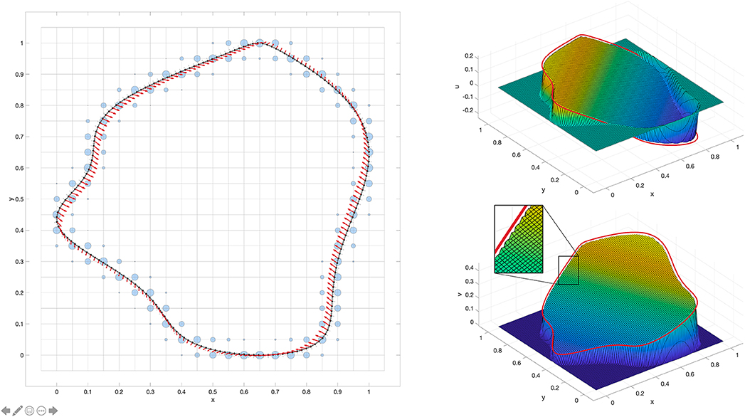
Figure 2. Raw results for the displacements of an arbitrary shape. The shape is cut out of a rectangular body (see left graph in Figure 1) with uniformly distributed loads σ_A = −0.8, σ_B = 0.1, and σ_C = 0.7. For the elastic parameters it was chosen ν = 0.3 and μ = 1. The stress distribution on the boundary of the shape is shown with the red arrows in the left image. The blue circles show the weights which result from the Lagrange polynomials used for the bilinear interpolations necessary for the convolution (for details see the main text of this section). The colored images on the right show the raw results for the displacements u and v obtained with the convolution. The red line represents the analytical solution for the displacements on the boundary of the shape. Note that the resolution of both the boundary and the FFT grid is chosen lower in the image on the left than in the results on the right merely for the purpose of a better visualization.

FIGURE 3

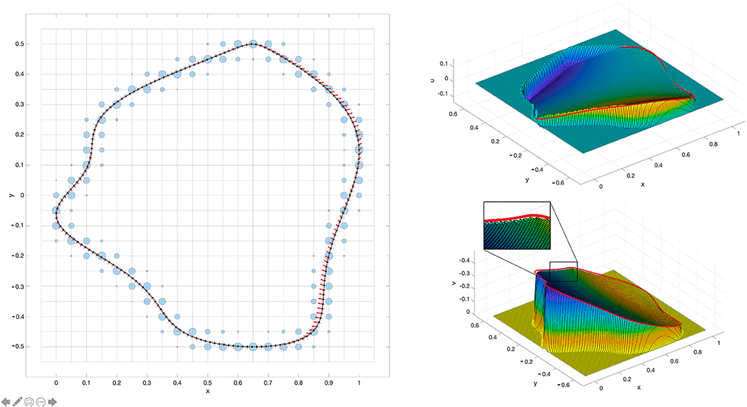
Figure 3. Raw results for the displacements of an arbitrary shape. The results are displayed as in Figure 2, here however the shape is cut out of a rectangular beam (see right graph in Figure 1) with an end load F = 0.2 and dimensions a = 1 and b = 0.5. For the elastic parameters it was chosen ν = 0.3 and μ = 1.

So far we have used the analytical values of both the tractions and displacements on the boundary in order to obtain the FFT raw results. Let us now consider a problem where we only set the tractions on the boundary and seek a numerical solution for the displacements on the boundary. Figure 4 shows the results of such a procedure for different cutouts from the uniformly loaded rectangular body. A conjugate gradient method with 10 iterations is used to solve for the displacements on the boundary. Therein, the projection of the FFT results onto the actual boundary is performed via bilinear interpolation. Furthermore, nearby panel interactions were calculated directly in a radius of 7 panels in order to eliminate oscillations. It can be observed that the method converges well to the analytical results for all three exemplary shapes.

FIGURE 4

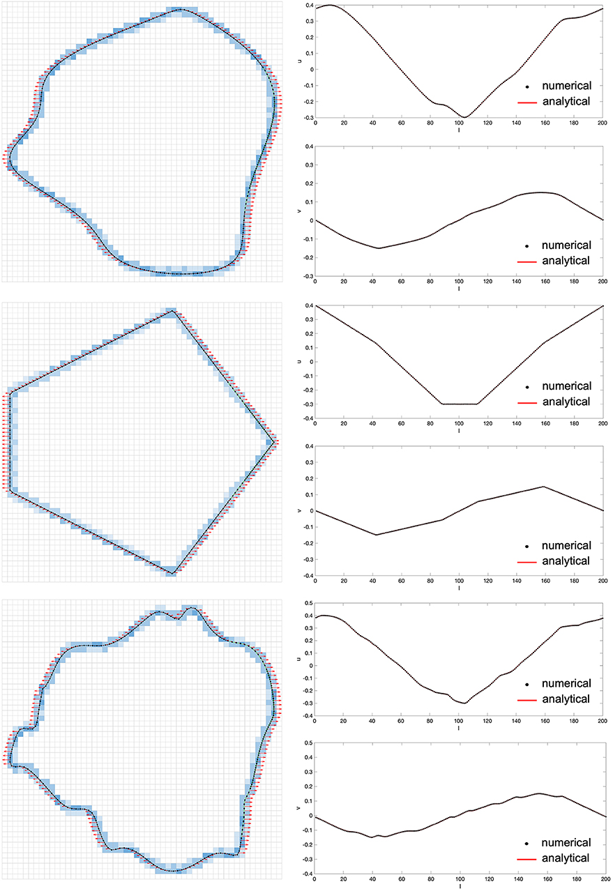
Figure 4. Results for the boundary displacements of three different cutouts from a rectangular body (see left graph in Figure 1) with a uniformly distributed load σ_A = 1, σ_B = 0, and σ_C = 0. For the elastic parameters it was chosen ν = 0.3 and μ = 1. The given stress distribution on the boundary is displayed with red arrows (left images), and the numerical results for the displacements on the boundary are shown in the diagrams on the right with black dots plotted over the analytical solution. l denotes the number of the equally spaced boundary nodes.

Variable FFT Grid

As we have observed in the previous section, the raw FFT data is highly accurate at a distance to the boundary but begins to oscillate in close proximity to the boundary. Consequently, the small number of nearby panel interactions is calculated directly in the pFFT technique and the larger number of all remaining panel interactions is computed with the FFT. Let us stress the point of having these two levels of accuracy. Then the question arises, why one does not use a hierarchy with even more levels of accuracy. Examining Figures 2–4, it seems obvious that the large number of unused discretization points of the FFT grid where no interpolation weights are placed are a waste of computational power. There are no numerical values at these points except zeros, and we have no interest in the results at these points after the convolution was applied. Philips and White addressed this by using an FFT grid which is coarser than the actual discretization of the boundary. This is enabled by using higher order interpolation techniques. A different or even additional approach might be a refinement of the grid at the boundary, see Figure 5. The main question which arises with a variable grid is how to apply the FFT which requires a regular grid. In the following, we illustrate that an O(NlogN) algorithm seems technically feasible with this approach. Consider cutting the arbitrary shape shown in Figure 5 into segments and aligning them one after the other as shown in Figure 6. Repositioning the segments in such a way creates an almost “one-dimensional” arrangement when compared to the original two-dimensional shape. It is this reduction in dimension which we seek in order to lower the computational complexity. This new line of segments is longer than the circumference of the original shape because for each segment, we include some additional space around it (see Figure 6 and compare with Figure 5). This way, it is ensured that while we convolute the kernels over the line of segments, the influence of the segments among each other is excluded. Exemplary raw results from this technique are shown in Figure 7. First, the convolutions are obtained on the rough grid level. From these results, we then subtract the influence obtained with the convolutions on the line of segments using also the rough grid level. Then, we add the influence of the convolutions over the line of segments using the fine grid level to our results using bilinear interpolation. Qualitatively, it can be observed that the results on the fine grid close to the boundary appear similar to the results which were obtained with the significantly more expensive technique used in Figure 2. This brief example can be regarded as a first sketch to indicate feasibility of the concept.

FIGURE 5

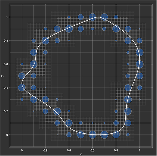
Figure 5. An arbitrary shape fully enclosed with a grid which is refined in close proximity to the boundary of the shape. The blue dots represent the weights of the Lagrange polynomials used for the bilinear interpolation of the boundary values with the coarse grid.

FIGURE 6

Figure 6. Segments of the arbitrary shape displayed in Figure 5 aligned one after the other. Each segment (fine bright grid) is chosen with some additional space around it (fine dark grid) so as to assure that the segments do not influence each other upon convolution with the kernels.

FIGURE 7

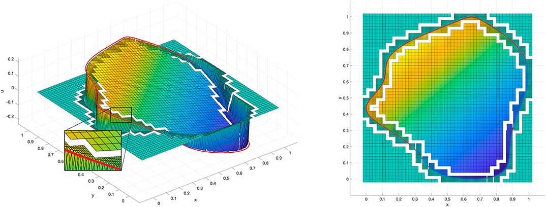
Figure 7. Exemplary raw results for the displacement component u obtained on a grid with two discretization levels for the same problem as it is displayed in Figure 2 with a single regular grid. The results on the fine grid level close to the boundary (the analytical solution is displayed with the red line) appear similar to the results which were obtained with the significantly more expensive technique used in Figure 2. The white borders between the two discretization levels are displayed for the purpose of a better visualization of the two discretization levels.

Conclusion

In this work, the pFFT was applied to solve the 2D Navier equation on arbitrary two-dimensional shapes. Furthermore, it was illustrated how the pFFT technique might be extended in order to decrease its computational complexity. In the standard pFFT approach, all panel influences which are not calculated directly are obtained on a single regular grid. In the present study, a variable gird was suggested to obtain these influences. It was outlined how it is possible to apply the FFT on each level of this variable grid by rearranging segments of the shape. A brief example was presented which indicates feasibility of the concept. However, more studies will be needed to research this concept further. Open questions include how to choose the grid size and number of levels of the variable grid, how high the order of the interpolation techniques used for projection onto the variable grid should be, how best to realize the interpolation between the grid levels, how the variable grid will influence iterative the solvers, and finally how the computational complexity and accuracy of the method compare to the standard pFFT technique and other methods designed to accelerate the Boundary Element Method.

Data Availability Statement

The original contributions presented in the study are included in the article/supplementary materials, further inquiries can be directed to the corresponding author/s.

Author Contributions

The author confirms being the sole contributor of this work and has approved it for publication.

Conflict of Interest

The author declares that the research was conducted in the absence of any commercial or financial relationships that could be construed as a potential conflict of interest.

Acknowledgments

The author would like to thank V. L. Popov and M. Heß for valuable discussions on the topic and critical comments.

References

Anderson, J. (2017). Fundamentals of Aerodynamics. New York, NY: McGraw-Hill.

PubMed Abstract | Google Scholar

Barber, J. (2004). Elasticity. Ann Arbor, MI: Kluwer Academic Publishers. doi: 10.1007/0-306-48395-5

CrossRef Full Text | Google Scholar

Benad, J. (2015). The Flying V - A new aircraft configuration for commercial passenger transport. Deutscher Luft- und Raumfahrtkongress 2015 (Rostock). 101.

Google Scholar

Benad, J. (2018). Efficient calculation of the BEM integrals on arbitrary shapes with the FFT. Facta Universitatis, Series Mechan. Eng. 16, 405–417. doi: 10.22190/FUME180912034B

CrossRef Full Text | Google Scholar

Benad, J. (2019). Numerical methods for the simulation of deformations and stresses in turbine blade fir-tree connections. Facta Universitatis, Series Mechan. Eng. 17, 1–15. doi: 10.22190/FUME190103008B

CrossRef Full Text | Google Scholar

Benedetti, I., Aliabadi, M., and Davi, G. (2008). A fast 3D dual boundary element method based on hierarchical matrices. Int. J. Solids Struc. 45, 2355–2376. doi: 10.1016/j.ijsolstr.2007.11.018

CrossRef Full Text | Google Scholar

Cheng, A., and Cheng, D. (2005). Heritage and early history of the boundary element method. Eng. Anal. Bound. Elem. 29, 268–302. doi: 10.1016/j.enganabound.2004.12.001

CrossRef Full Text | Google Scholar

Faggiano, F., Vos, R., Baan, M., and Van Dijk, R. (2017). Aerodynamic design of a flying v aircraft. 17th AIAA aviation technology. Integr. Operat. Conf. 6:3589. doi: 10.2514/6.2017-3589

CrossRef Full Text | Google Scholar

Galin, L. (2008). “Plane elasticity theory,” in Contact Problems, ed G. Gladwell (Dordrecht: Springer). doi: 10.1007/978-1-4020-9043-1_2

CrossRef Full Text | Google Scholar

Gaul, L., and Fiedler, C. (2013). Methode der Randelemente in Statik und Dynamik. Berlin: Springer. doi: 10.1007/978-3-8348-2537-7

CrossRef Full Text | Google Scholar

Gross, D., Hauger, W., and Wriggers, P. (2014). Technische Mechanik 4. Berlin: Springer. doi: 10.1007/978-3-642-41000-0

CrossRef Full Text | Google Scholar

Hahn, H. (1985). Elastizitätstheorie. Wiesbaden: Vieweg Teubner Verlag. doi: 10.1007/978-3-663-09894-2

CrossRef Full Text | Google Scholar

Irgens, F (Ed.). (2008). “Theory of elasticity,” in Continuum Mechanics (Berlin: Springer). doi: 10.1007/978-3-540-74298-2

CrossRef Full Text | Google Scholar

Katz, J., and Plotkin, A. (2001). Low-Speed Aerodynamics. Cambridge: Cambridge University Press. doi: 10.1017/CBO9780511810329

CrossRef Full Text | Google Scholar

Kelly, P. (2013). “Linear Elasticity,” in An introduction to Solid Mechanics (Lecture Notes) (University of Auckland). Available online at: http://homepages.engineering.auckland.ac.nz/~pkel015/SolidMechanicsBooks/How_to_reference.htm

Li, Q., Voll, L., Starcevic, J., and Popov, V. L. (2018). Heterogeneity of material structure determines the stationary surface topography and friction. Sci. Rep. 8:32545.doi: 10.1038/s41598-018-32545-5

PubMed Abstract | CrossRef Full Text | Google Scholar

Lim, K., He, X., and Lim, S. (2008). Fast Fourier transform on multipoles (FFTM) algorithm for Laplace equation with direct and indirect boundary element method. Comput. Mechan. 41, 313–323. doi: 10.1007/s00466-007-0187-5

CrossRef Full Text | Google Scholar

Masters, N., and Ye, W. (2004). Fast BEM solution for coupled electrostatic and linear elastic problems. NSTI Nanotech 2, 426–429. doi: 10.1016/j.enganabound.2004.02.001

CrossRef Full Text | Google Scholar

Müser, M., Dapp, W., Bugnicourt, R., Sainsot, P., Lesaffre, N., Lubrecht, T., et al. (2017). Meeting the contact-mechanics challenge. Tribol. Lett. 65:118. doi: 10.1007/s11249-017-0900-2

CrossRef Full Text | Google Scholar

Paggi, M., and Hills, D. (2020). Modeling and Simulation of Tribological Problems in Technology. Udine: Springer. doi: 10.1007/978-3-030-20377-1

CrossRef Full Text | Google Scholar

Palermo, M., and Vos, R. (2020). Experimental aerodynamic analysis of a 4.6%-scale flying-v subsonic transport. AIAA Scitech 2020 Forum, 2228. doi: 10.2514/6.2020-2228

CrossRef Full Text | Google Scholar

Phillips, J. (1997). Rapid solution of potential integral equationsin complicated 3-dimensional geometries. (Doctoral thesis). Massachusetts Institute of Technology , Cambridge, MA, United States.

Phillips, J., and White, K. (1997). A precorrected FFT-method for electrostatic analysis of complicated 3-D structues. IEEE Trans. Comput Aided Des. Integr. Circ. Syst. 16, 1059–1072. doi: 10.1109/43.662670

CrossRef Full Text | Google Scholar

Pohrt, R., and Li, Q. (2014). Complete Boundary Element Formulation for Normal and Tangential Contact Problems. Phys. Mesomechan. 17, 334–340. doi: 10.1134/S1029959914040109

CrossRef Full Text | Google Scholar

Popov, V. L. (2017). Contact Mechanics and Friction. Berlin: Springer. doi: 10.1007/978-3-662-53081-8

CrossRef Full Text | Google Scholar

Popov, V. L., Pohrt, R., and Li, Q. (2017). Strength of adhesive contacts: Influence of contact geometry and material gradients. Friction 5, 308–325. doi: 10.1007/s40544-017-0177-3

CrossRef Full Text | Google Scholar

Putignano, C., Afferrante, L., Carbone, G., and Demelio, G. (2012). A new efficient numerical method for contact mechanics of rough surfaces. Int. J. Solids Struc. 49, 338–343. doi: 10.1016/j.ijsolstr.2011.10.009

CrossRef Full Text | Google Scholar

Raymer, D. (2018). Aircraft Design: A Conceptual Approach. Reston, VA: American Institute of Aeronautics and Astronautics, Inc. doi: 10.2514/4.104909

CrossRef Full Text | Google Scholar

Rubio Pascual, B., and Vos, R. (2020). The effect of engine location on the aerodynamic efficiency of a flying-v aircraft. AIAA Scitech 2020 Forum 1954. doi: 10.2514/6.2020-1954

CrossRef Full Text | Google Scholar

Smith, A. (1990). The panel method: Its original development. Appl. Comput. Aerodynam. 125, 3–17. doi: 10.2514/5.9781600865985.0003.0017

CrossRef Full Text | Google Scholar

Willis, D., Peraire, J., and White, J. (2006). A combined pFFT-multipole tree code, unsteady panel method with vortex particle wakes. Int. J. Num. Methods fluids 53, 1399–1422. doi: 10.1002/fld.1240

CrossRef Full Text | Google Scholar