FFT-Based Methods for Computational Contact Mechanics

Introduction

Contact of materials is a common engineering phenomenon, and the solution to a contact problem, in terms of pressure, deformations, and stresses, as well as flash temperature, is usually among first steps in the design and analysis of an engineering system or a functional device. A contact problem is solved first for the information of the contacting interface, such as contact pressure, surface interaction, contact area, and interfacial friction, followed by a boundary-value solution process for the stresses in each contacting body. At least two sets of convolutions, each for a group of excitations and Green's functions, are involved, i.e., displacements and stresses, in response to surface tractions, and the former are calculated first (Conry and Seireg, 1971; Kalker and van Randen, 1972; Kalker, 1986; Polonsky and Keer, 1999). When solving the contact of bodies involving an inclusion-containing material, the mathematical correlation between an eigenstrain and a Green's function appears (Liu et al., 2012). In most cases, the convolution nature makes it possible to formulate and solve a contact problem by means of an efficient fast Fourier transform (FFT) algorithm (Ju and Farris, 1996; Stanley and Kato, 1997; Ai and Sawamiphakdi, 1999; Hu et al., 1999; Polonsky and Keer, 1999, 2000; Liu et al., 2000; Liu and Wang, 2002). We will discuss and summarize the theories, algorithms, and numerical methods of FFT-based contact modeling approaches.

If the contact body can be treated as a mathematically “semi-infinite” medium, or a half-space material, analytical influence coefficients (ICs), or frequency-response functions (FRFs), may be derived for certain problems. Normally such a simplification can be made if deformations are small and the radii of curvature of contact bodies are sufficiently larger than the effective contact size of these two bodies. In the case of the macroscopic contact of two spheres, or two cylinders, of the same size and material, if the contact radius, or half width, a, is 10% of the radius of the contact body, the maximum error from using the z-direction deformation to replace the radial deformation at the contact edge is within 0.5%. However, stresses need more attention. Two contact problems, (1) two steel spheres of the same radius and (2) their equivalent sphere and a half space, are analyzed using the finite-element method (FEM) without considering plasticity. Figure 1 shows maximum relative errors of the von Mises stress along the central axis, due to ignoring curvature, as a function of a/R_e. The error is about 7% when a/R_e reaching 10%, and this situation is beyond the “small elastic deformation” assumption. In the elastic range, using steels as an example, the maximum error of the von Mises stress is <3% if the half-space solution is pursued. Similar small errors due to the use of the half-space assumption in the elastic range have also been reported by Londhe et al. (2018), in the comparison of the results from the FEM and Hertz formulas for different types of contacts.

FIGURE 1

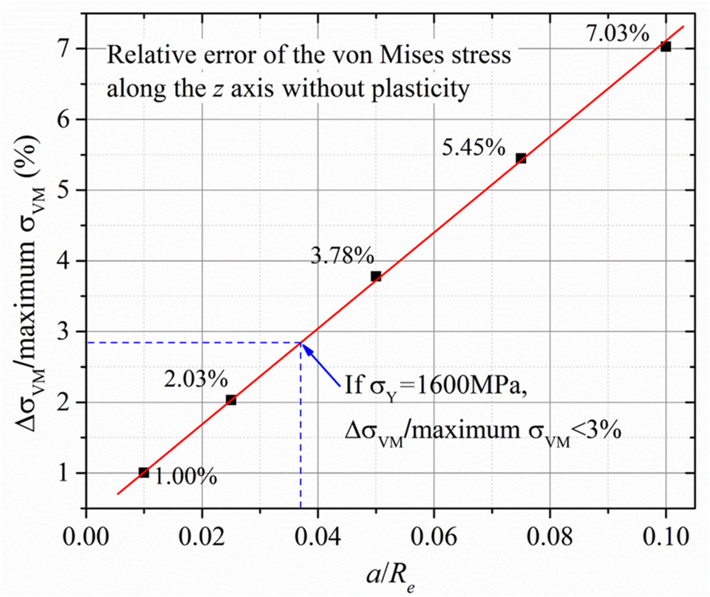
Figure 1. Maximum errors of the von Mises stress, σ_VM, along the z axis, or the central axis in the depth direction, by using the half-space approach to solve the problem of contact of two equal spheres, without considering plasticity, calculated with the FEM; a is the half contact width, R_e is the equivalent radii of the contact bodies, and 1/R_e = 1/R₁ + 1/R₂.

In a contact simulation, the computational complexity of evaluating a convolution via direct summation of the products of ICs and surface traction is on the order of O(N²), where N is the mesh number. If N is large and the convolution has to be repeatedly calculated in an iteration process, the computation burden is very heavy. The works by Ju and Farris (1996), Nogi and Kato (1997), Stanley and Kato (1997), Ai and Sawamiphakdi (1999), Hu et al. (1999), Polonsky and Keer (2000), and Liu et al. (2000) are in a chain of studies to apply the FFT to evaluate the convolutions for elastic deformation and stresses efficiently in the field of contact mechanics and tribology. Several papers have reviewed such efforts of solving tribology problems via the FFT and analyzed the sources of errors (Liu et al., 2000; Wang et al., 2003; Liu S. et al., 2007; Wang and Zhu, 2019). Although most of the effort is on solving non-conformal contact problems, the FFT methods suit for certain conformal-contact problems as well if they involve a convolution and have ICs obtained analytically or numerically. Actually, the circular nature of a cylindrical structure fits the circular convolution theorem perfectly. Liu and Chen (2012) and Liu (2013) reported an FFT-based conformal-contact model for two-dimensional (2D) problems. Wang and Jin (2004) conducted the fluid-film lubrication analysis for artificial joints, which requires the determination of the elastic deformation of the bearing surface of both the acetabular cup and the femoral head. They used FFT along with the spherical distance and numerical ICs from an FEM calculation.

The FFT methods greatly help reduce the computation burden. For example, for a three-dimensional (3D) point-contact problems, the FFT operation is on the order of O(12Nlog₂ [4N]), to be discussed in detail later. Its ratio to the operation needed for calculating the convolution is 12Nlog₂ (4N)/N² = 12log₂(4N)/N = 0.00024, if N is 1024^*1024. This is a significant saving of computational time. The key issues to be addressed are (1) how should the Fourier transform (FT) method be properly used to solve contact problems? (2) Can one solution algorithm be used for all problems?

Theoretically, the Fourier transform can be used for infinite-domain and the Fourier series for periodic problems, but most contact problems do not satisfy these conditions. For example, a point-contact problem has its pressure only on a small region of contacting surfaces. If the FFT is directly used to solve such a problem, the results near the borders have notable errors. In order to reduce the periodicity error, Ju and Farris (1996) substantially extended the domain, Ai and Sawamiphakdi (1999) decomposed the total pressure into a smooth portion and a zero-mean fluctuating portion, and Polonsky and Keer (2000) developed a hybrid algorithm by adding a special correction procedure. Each of these brings in a certain accuracy improvement while introducing new complications. We have investigated the theories of contact mechanics and signal analyses, and realized that proper convolution theorems should be considered in solving different contact problems of non-conformal and conformal configurations (Figure 2) (Liu et al., 2000; Liu and Wang, 2002; Liu S. et al., 2007; Liu and Hua, 2009; Liu and Chen, 2012), as summarized by Wang and Zhu (2019, Chapter 4).

FIGURE 2

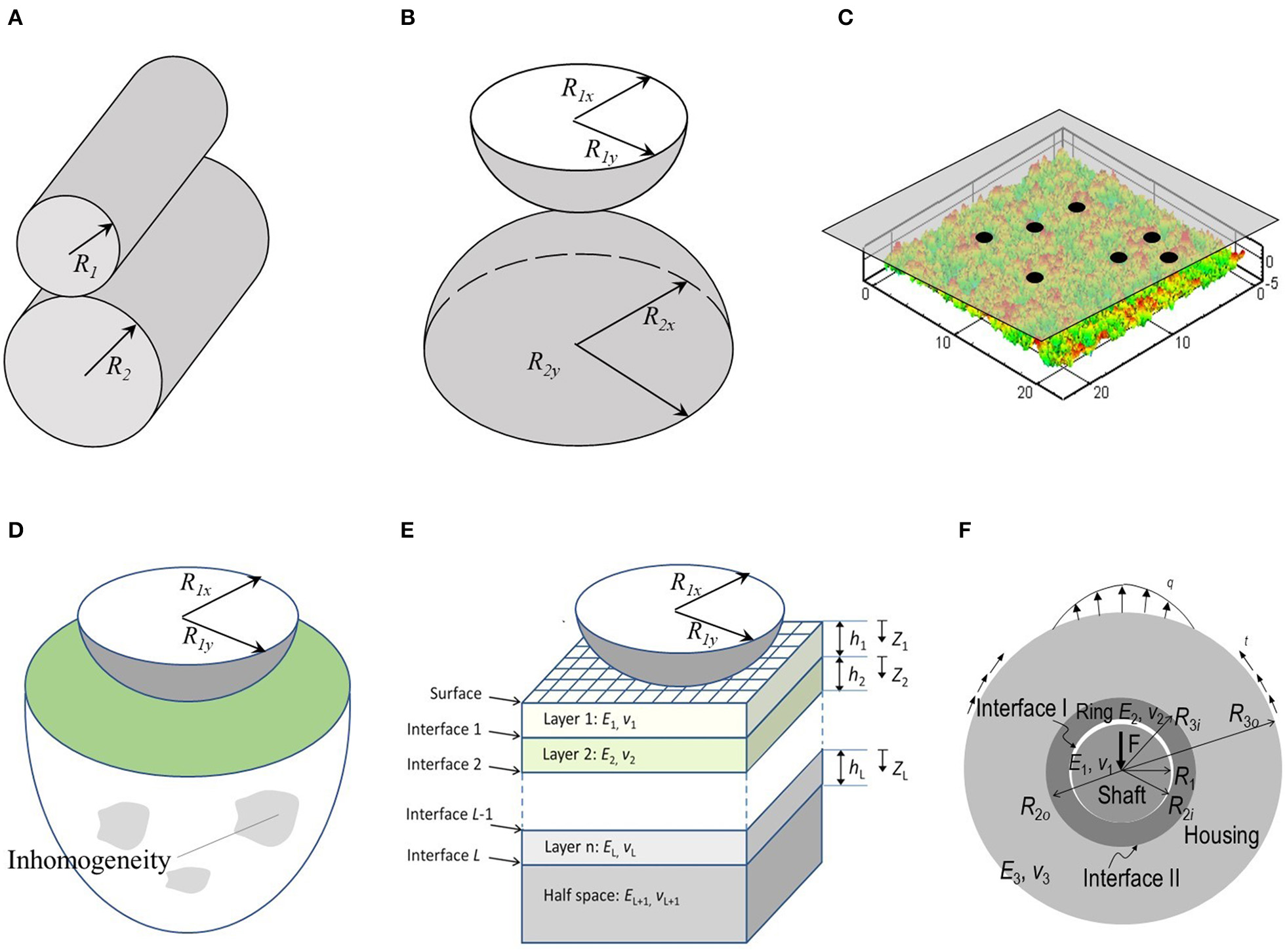
Figure 2. Different types of contact problems solved by using a FFT-based method. (A) Line contact, (B) point contact, (C) nominally flat-flat contact, (D) contact involving an inhomogeneous material, (E) contact involving a layered material or other anisotropic materials, and (F) conformal contact of 2D journal bearings or rollers. Note that all surfaces can be smooth or rough.

In this paper, we will discuss the basic issues of the FFT methods for contact analyses from the convolution theorems and the tree of the Fourier-transform algorithms for solving different contact problems, such as (1) the algorithm of discrete-convolution and fast-Fourier-transform (DC-FFT), with double domain extension in each dimension, for non-periodic problems, and the discrete-convolution and fast-Fourier-transform algorithm (DC-FFT) without domain extension for journal bearing problems, (2) the algorithm of continuous-convolution and Fourier-transform (CC-FT) for periodic (or infinite) contact problems, (3) the algorithm of discrete convolution with duplicated padding and FFT (DCD-FFT), that of discrete-continuous convolutions and FFT (DC-CC-FFT), and that of the discrete convolution with IC summation and FFT (DCS-FFT) for 3D line-contact problems that are periodic (or infinite) in one direction but non-periodic in the other direction, (4) the algorithm of discrete-correlation and FFT (DCR-FFT) for inclusion problems, (5) the FRF-IC conversion method, as well as the applications of them to solve the contact problems involving layered materials, anisotropic elastic materials, and viscoelastic polymers, or those subjected to multifields, and (6) a non-uniform DCS-FFT method, recently developed by Sun et al. (2020), for solve large-scale contact problems. Most of the contents in this paper are based on the works by Liu et al. (2000, 2002), Liu and Wang (2002), Boucly et al. (2005), Chen et al. (2008), Liu and Hua (2009), Yu et al. (2014, 2016), Zhang X. et al. (2017, 2018), Zhang and Wang (2019), Sun (2020), Sun et al. (2020), Zhang et al. (2020a,b), and Chapter 4 in the book by Wang and Zhu (2019). Table 1 summarizes the FFF-based approaches and their applications. It should be mentioned that the pressure and contact area that satisfy the Kuhn-Tucker type complementary conditions can be solved with different methods, and the conjugate gradient method (CGM) (Polonsky and Keer, 1999; Jin et al., 2013) is currently the widely accepted one.

TABLE 1

Table 1. FFT methods for contact analyses.

In the following, the elastic field means the distributions of stresses and displacements, and the target domain means the physical domain, on which a physical contact problem is defined. The algorithms and methods will be explained mainly through deformation calculations; details of the FFT-based computations of stresses, flash temperature, and other physical fields can be found in the reports by Liu (2001), Liu and Wang (2002), Chen et al. (2008), Zhang X. et al. (2018), and Wang and Zhu (2019), as well as those mentioned in the previous paragraph.

Convolution, Frequency Response Function, and Influence Coefficients

Convolution and ICs

Let's use the pressure-displacement relationships, such as the Flamant and Boussinesq equations (Johnson, 1987), as examples. Here, an excitation at ξ, or (ξ, η), and a response at x, or (x, y), are related to each other through a Green's function defined with the distance between the two, which is either |x − ξ| or $R^I=\sqrt{{\left(x-\xi \right)}^2+{\left(y-\eta \right)}^2}.$

The surface normal displacement of a cylinder in a line contact, $u_z(x)$, due to pressure p(x) on surface region S_x is

$\begin{array}{ll}{u}_z(x)=-\frac{4}{\pi E^{\prime }}{\displaystyle \underset{S_x}{\int }\text{ln}|x-\xi |p(\xi )d\xi }=C{\displaystyle \underset{S_x}{\int }G(x-\xi )p(\xi )d\xi }& (1)\end{array}$

where C = −4/(πE′), E' is the effective Young's modulus and the corresponding Green's function is Cln |x|. The integral kernel, G, is defined as

$\begin{array}{ll}G(x)=\text{ln}|x|& (2)\end{array}$

In numerical modeling, the equation above can be discretized and re-written as the summation of the products of influence coefficients D(k, i), or D_i,j, and nodal pressures P_i.

$\begin{array}{ll}{u}_z(x_k)=C{\displaystyle \sum _{i=1}^{N_p}D(k,i)p_i=C{\displaystyle \sum _{i=1}^{N_p}{D}_{k,i}{p}_i},(k=1,2,3,...N_d)}& (3)\end{array}$

where N_p, N_d are the total numbers of nodes for pressure and deformation, respectively.

A shape function, Ys, may be used to distribute pressure, or other excitations, around a nodal point, and the commonly used shape functions are 0-order, 1st-order, and 2nd-order polynomials. Detailed expressions and use of these shape functions can be found in the book by Wang and Zhu (2019).

The ICs are from the elementary integration of Green's function and shape function Ys, implying unit nodal pressure, or from G and shape function Ys without including coefficient C. The latter is used here. In general,

$\begin{array}{ll}D(k,i)={\displaystyle \underset{x_l=x_i-{\Delta }_2-x_k}{\overset{x_u=x_i+{\Delta }_1-x_k}{\int }}G(x_k-{\xi }_i)Ys({\xi }_i)d\xi }=\left\{f(x_u)-f(x_l)\right\}& (4)\end{array}$

where f is the integration result, and x_u and x_l are the upper and lower boundaries of the element integration at x_i, with Δ₁ and Δ₂ marking the element size.

If the zero-order shape function is used, the influence coefficient expression becomes

$\begin{array}{l}D(k,i)=\left(x_{i+1/2}-x_k\right)\left(\text{ln}|x_{i+1/2}-x_k|\right)-\left(x_{i-1/2}-x_k\right)\left(\text{ln}|x_{i-1/2}-x_k|\right)\\ +(x_{i-1/2}-x_{i+1/2})& (5)\end{array}$

Note that here the influence coefficients, D, depend only on the geometric factors of the grid. When a uniform grid is used with the constant mesh spacing x_i+1-x_i = x_i-x_i−1 = 2Δ, the above becomes

$\begin{array}{l}D(k,i)=\left(x_i+\Delta -x_k\right)\left(\text{ln}|x_i+\Delta -x_k|\right)-\left(x_i-\Delta -x_k\right)\left(\text{ln}|x_i-\Delta -x_k|\right)\\ -2\Delta & (6)\end{array}$

For point-contact problems, surface normal displacement $u_z(x,y)$ due to pressure p(x, y) on surface area Ω is,

$\begin{array}{l}{u}_z(x,y)=\frac{2}{\pi E^{\prime }}{\displaystyle \underset{\Omega }{\iint }\frac{p(\xi ,\eta )}{\sqrt{{(x-\xi )}^2+{(y-\eta )}^2}}}d\xi d\eta \\ =C{\displaystyle \underset{\Omega }{\iint }\frac{p(\xi ,\eta )}{\sqrt{{(x-\xi )}^2+{(y-\eta )}^2}}}d\xi d\eta & (7)\end{array}$

where $C=\frac{2}{\pi E^{\prime }}$, G is from Green's function, defined as $G=\frac{1}{\sqrt{x^2+y^2}}$.

Likewise, the equation above can be re-written as the summation of the products of influence coefficients $D_{i,j}^{k,l}$ and nodal pressures p_i,j. The ICs are from the elementary integration of Green's function and a shape function, Ys, or G and shape function Ys without including the material properties, and the latter is used here.

$\begin{array}{ll}{u}_z(x_k,y_l)=C{\displaystyle \sum _{i=1}^{N_{px}}{\displaystyle \sum _{j=1}^{N_{py}}{D}_{i,j}^{k,l}{p}_{i,j}}}(k=1,2\dots N_{dx},l=1,2\dots N_{dy})& (8)\end{array}$

where N_dx, N_dy are the total numbers of nodes for deformation in the x, y directions, and N_px, N_py are the total numbers of nodes for pressure in the x, y directions, respectively.

$\begin{array}{ll}{D}_{i,j}^{k,l}={\displaystyle \underset{x_l}{\overset{x_u}{\int }}{\displaystyle \underset{y_l}{\overset{y_u}{\int }}G(x_k,y_l,{\xi }_i,{\eta }_j)Ys({\xi }_i,{\eta }_j)d\xi d\eta }}& (9)\end{array}$

$\begin{array}{ll}\text{Or }D={\displaystyle \sum _{Elemental-contribution}\left\{f(x_u,y_u)+f(x_l,y_l)-f(x_u,y_l)-f(x_l,y_u)\right\}}& (10)\end{array}$

where f is the integration result, and (x_u, y_u) (x_l, y_l) are the upper and lower boundaries of the element integration.

If the zero-order shape function is used, the influence coefficient expression is (Love, 1929),

$\begin{array}{l}{D}_{i,j}^{k,l}=(x_k-x_i+a)\text{ln}\left[\frac{(y_l-y_j+b)+\sqrt{{(y_l-y_j+b)}^2+{(x_k-x_i+a)}^2}}{(y_l-y_j-b)+\sqrt{{(y_l-y_j-b)}^2+{(x_k-x_i+a)}^2}}\right]\\ +(y_l-y_j+b)\text{ln}\left[\frac{(x_k-x_i+a)+\sqrt{{(y_l-y_j+b)}^2+{(x_k-x_i+a)}^2}}{(x_k-x_i-a)+\sqrt{{(y_l-y_j+b)}^2+{(x_k-x_i-a)}^2}}\right]\\ +(x_k-x_i-a)\text{ln}\left[\frac{(y_l-y_j-b)+\sqrt{{(y_l-y_j-b)}^2+{(x_k-x_i-a)}^2}}{(y_l-y_j+b)+\sqrt{{(y_l-y_j+b)}^2+{(x_k-x_i-a)}^2}}\right]\\ +(y_l-y_j-b)\text{ln}\left[\frac{(x_k-x_i-a)+\sqrt{{(y_l-y_j-b)}^2+{(x_k-x_i-a)}^2}}{(x_k-x_i+a)+\sqrt{{(y_l-y_j-b)}^2+{(x_k-x_i+a)}^2}}\right]& (11)\end{array}$

Replacing x_k−i = x_k−x_i and y_l−j = y_l−y_j leads to the following.

$\begin{array}{l}{D}_{i,j}^{k,l}=\left(x_{k-i}+a\right)\text{ln}\left[\frac{\left(y_{l-j}+b\right)+\sqrt{{\left(y_{l-j}+b\right)}^2+{\left(x_{k-i}+a\right)}^2}}{\left(y_{l-j}-b\right)+\sqrt{{\left(y_{l-j}-b\right)}^2+{\left(x_{k-i}+a\right)}^2}}\right]\\ +\left(y_{l-j}+b\right)\text{ln}\left[\frac{\left(x_{k-i}+a\right)+\sqrt{{\left(y_{l-j}+b\right)}^2+{\left(x_{k-i}+a\right)}^2}}{\left(x_{k-i}-a\right)+\sqrt{{\left(y_{l-j}+b\right)}^2+{\left(x_{k-i}-a\right)}^2}}\right]\\ +\left(x_{k-i}-a\right)\text{ln}\left[\frac{\left(y_{l-j}-b\right)+\sqrt{{\left(y_{l-j}-b\right)}^2+{\left(x_{k-i}-a\right)}^2}}{\left(y_{l-j}+b\right)+\sqrt{{\left(y_{l-j}+b\right)}^2+{\left(x_{k-i}-a\right)}^2}}\right]\\ +\left(y_{l-j}-b\right)\text{ln}\left[\frac{\left(x_{k-i}-a\right)+\sqrt{{\left(y_{l-j}-b\right)}^2+{\left(x_{k-i}-a\right)}^2}}{\left(x_{k-i}+a\right)+\sqrt{{\left(y_{l-j}-b\right)}^2+{\left(x_{k-i}+a\right)}^2}}\right]& (12)\end{array}$

where a and b are the half length of the rectangular integration element.

Frequency Response Functions and ICs

The Fourier transform can be applied to the IC matrix, D, Equation (4), to obtain,

$\begin{array}{ll}\tilde{D}=\tilde{G}·\tilde{Y}s& (13)\end{array}$

$\begin{array}{ll}\text{and }\tilde{G}=\tilde{D}/\tilde{Y}s& (14)\end{array}$

where $\tilde{G}$ is the frequency response function excluding the elastic parameter, C. These two equations show how to obtain one from the other.

If discrete Fourier transform $\widehat{D}$ has already been obtained from a set of known ICs via the FFT, $\tilde{G}$ can be solved from $\tilde{G}=\tilde{D}/\tilde{Y}s$ once Fourier series coefficients $\tilde{D}$ can be obtained from $\widehat{D}$. Based on the sampling theorem, the one-dimensional (1D) relationship between the FT (~) and discrete Fourier transform (DFT) (^∧) of the ICs, sampled with mesh interval 2Δ, can be obtained as

$\begin{array}{l}{\widehat{D}}_i=\frac{1}{2\Delta }{\displaystyle \sum _{r=-\infty }^{\infty }\tilde{D}\left(\frac{2\pi i}{n·2\Delta }-\frac{2\pi r}{2\Delta }\right)}=\frac{1}{2\Delta }{\displaystyle \sum _{r=-\infty }^{\infty }\tilde{D}\left(\frac{\pi i}{n\Delta }-\frac{\pi r}{\Delta }\right)}\\ (i=0,1,2\cdots ,n-1)& (15)\end{array}$

An aliasing control parameter, AL, can be introduced instead of summation for r from –∞ to ∞, in order to satisfy a required accuracy while saving computation time.

$\begin{array}{l}{\widehat{D}}_i=\frac{1}{2\Delta }{\displaystyle \sum _{r=-AL}^{AL}\tilde{D}\left(\frac{2\pi i}{n·2\Delta }-\frac{2\pi r}{2\Delta }\right)}=\frac{1}{2\Delta }{\displaystyle \sum _{r=-AL}^{AL}\tilde{D}\left(\frac{\pi i}{n\Delta }-\frac{\pi r}{\Delta }\right)}\\ (i=0,1,2\cdots ,n-1)& (16)\end{array}$

The above can be simplified if the sampling frequency is sufficiently high, or the datum interval is sufficiently small.

$\begin{array}{ll}{\widehat{D}}_i\approx \frac{1}{2\Delta }\tilde{D}\left(\frac{2\pi i}{n·2\Delta }\right)=\frac{1}{2\Delta }\tilde{D}\left(\frac{\pi i}{n\Delta }\right)(i=0,1,2\cdots ,n-1)& (17)\end{array}$

The above becomes exact if and only if $m_s>2m_{\max }$ (Morrison, 1994) with $\pm m_{\max }$ as the band limit (or $m_{\max }$ as the highest frequency component), beyond which there is no Fourier transform results (Walker, 1996). Then, only the term at r = 0 is needed.

Likewise, the 2D relationship between the FT (~) and DFT (^∧) of the ICs is

$\begin{array}{l}{\widehat{\widehat{D}}}_{i,j}=\frac{1}{{\Delta }_x{\Delta }_y}{\displaystyle \sum _{r_x=-AL}^{r_x=AL}{\displaystyle \sum _{r_y=-AL}^{r_y=AL}\widetilde{\stackrel{~}{D}}}}(\frac{2\pi }{n_x{\Delta }_x}i-\frac{2\pi }{{\Delta }_y}{r}_y,\frac{2\pi }{n_y{\Delta }_y}j-\frac{2\pi }{{\Delta }_y}{r}_x)\\ (i=0,1,2\cdots ,n_x-1,j=0,1,2\cdots ,n_y-1)& (18)\end{array}$

where ${\Delta }_x$ and ${\Delta }_y$ are the mesh intervals in the x and y directions, and ${\Delta }_x={\Delta }_y=2\Delta$ if the meshes are uniform in both directions.

This means two operations. (1) Upon knowing $\tilde{D}$ from $\widehat{D}$ via Equations (17) or (18) with a properly chosen discretization interval, 2Δ < 2π/ω_max, we can solve $\tilde{G}$ using the equation below.

$\begin{array}{l}{\tilde{G}}_i=\tilde{G}\left(\frac{2\pi i}{n·2\text{Δ}}\right)=\tilde{D}\left(\frac{2\pi i}{n·2\Delta }\right)/\tilde{Y}\left(\frac{2\pi i}{n·2\Delta }\right)\\ \approx 2\Delta ·{\widehat{D}}_i/\tilde{Y}s\left(\frac{2\pi i}{n·2\Delta }\right)\\ =2\Delta ·{\widehat{D}}_i/\tilde{Y}s\left(\frac{\pi i}{n\Delta }\right)(i=0,1,2\cdots ,n-1)& (19)\end{array}$

(2) Upon knowing $\tilde{G}$, we can get $\widehat{D}$ from $\tilde{D}$ using Equations (13) and (17), or (18). In many cases where the solutions to frequency response functions are more convenient than those to Green's functions, and this operation can be utilized to convert the FRFs to the discrete Fourier transformed ICs.

Convolution Theorems

Equations (1) and (7) are both convolutions, which can be solved efficiently via Fourier transform followed by inverse Fourier transform. However, because the pressure may be in a discrete form, i.e., rough-surface contact pressure, and its application domain may be in different sizes, i.e., finite or infinite, accurate solutions to these equations, and others in the same nature, require the use of different convolution theorems. The following explains these theorems with 1D datum series for convenience.

Continuous Linear Convolution

If a set of continuous functions of t, f and G, follows the convolution in Equation (20), resulting in O, then the Fourier transform of the convolution results, $\tilde{O}(\omega )$, satisfies Equation (21), which convert the integration in Equation (20) to multiplication of continuous Fourier transforms of f and G.

$\begin{array}{ll}O(t)={\displaystyle {\int }_{-\infty }^{\infty }G(t-\tau )f(\tau )d\tau }\equiv G(t)*f(t)& (20)\end{array}$

$\begin{array}{ll}\tilde{O}(\omega )=\tilde{G}(\omega )\tilde{f}(\omega )& (21)\end{array}$

where O is accounted as the response of the continuous linear convolution, and symbol “*” is the convolution operator; $\tilde{O}(\omega )$, $\tilde{G}(\omega ),\tilde{f}(\omega )$ are Fourier transformed results of O, G, and f , with ω for frequency corresponding to the domain of variable t. The tilde (~), means a 1D Fourier transform. For contact problems, f can be the excitation force, such as pressure, if it is a continuous function defined in the entire domain, and G is Green's function, both are function of space variable x. Then, frequency ω is corresponding to the space domain.

Periodic Convolution

If D_p(i) and f_p(i) are periodic functions with period N, the product of their discrete Fourier series (DFS) coefficients, ${\stackrel{⌣}{D}}_p(m)$ and ${\stackrel{⌣}{f}}_p(m)$, with m for the frequency, is ${\stackrel{⌣}{O}}_p$ that can be expressed as (Oppenheim et al., 1999),

$\begin{array}{ll}{\stackrel{⌣}{O}}_p(m)={\stackrel{⌣}{D}}_p(m){\stackrel{⌣}{f}}_p(m)& (22)\end{array}$

The periodic sequence, O_p, with the same period, N, is the periodic convolution analyzed in one period, N, shown below.

$\begin{array}{ll}{(O_p)}_j={\displaystyle \sum _{r=0}^{N-1}}{(D_p)}_{j-r}{(f_p)}_{r}0\le j\le N-1& (23)\end{array}$

For contact problems, D_p(i) and f_p(i) are D_p(x_i) and f_p(x_i). Here, the subscript can be negative.

Cyclic (Circular) Convolution

Based on Oppenheim et al. (1999), if D_c(i) and f_c(i) are sequences of finite length N, and their DFT results are ${\widehat{D}}_c(m)$ and ${\widehat{f}}_c(m)$, with m for the frequency, then their term-by-term product is $\widehat{O}$_c, expressed as

$\begin{array}{ll}{\widehat{O}}_c(m)={\widehat{D}}_c(m){\widehat{f}}_c(m)& (24)\end{array}$

The finite sequence O_c is actually the circular convolution analyzed in length N, shown below.

$\begin{array}{ll}{(O_c)}_j={\displaystyle \sum _{r=0}^{N-1}}{(D_c)}_{j-r}{(f_c)}_{r}0\le j\le N-1& (25)\end{array}$

$\begin{array}{ll}\text{Or }{(O_c)}_j={\displaystyle \sum _{r=0}^{N-1}}{(D_c)}_{j-r+NH(r-j)}{(f_c)}_{r}0\le j\le N-1& (26)\end{array}$

where H(r-j) is the Heaviside unit step function, which is 1 when r-j is positive, or 0 otherwise. The term NH(r-j) contributes to the subscript numbering only when the step function is not zero to avoid negative subscript. Here, subscript -r reverses the sequence of the D series and subscript j shifts it in a circular fashion. More details has been given by Liu et al. (2000).

This means that the Fourier transform operation in Equation (24) is valid only when the convolution of D_c(i) and f_c(i) is in the form given in Equations (25) or (26). Although Equations (23) and (25) are for different events, they are expressed in the same form and lead to the same results in one period (Oppenheim et al., 1999).

The cyclic (circular) convolution is for series of finite lengths, and the circular fashion of the D series make it suitable for problems with either periodic features (e.g., nominally flat contact with a special IC treatment) or a circular configuration (e.g., cylindrical and journal bearing problems). Liu and Chen (2012) and Liu (2013) reported an FFT-based conformal-contact model for 2D problems with two concentric cylindrical interfaces, Figure 1F, for which we can directly apply the cyclic convolution theorem and 1D FFT operations to obtain the shaft deformation. However, for problems without the periodic features, such as counterformal line/point contact problems, special measures are needed to make the D series in such a needed circular fashion so that the cyclic convolution can be properly performed. The ICs and the pressure series can be properly handled based on the characteristics of the problems, e.g., Liu S. et al. (2000, 2007), Liu and Wang (2002), and Chen et al. (2008), so that they fit the need for the circular-convolution analyses. Because the FFT is a collection of algorithms for fast execution of DFT, the cyclic convolution of the two datum series (Equation 26) should also satisfy Equation (24) when the DFT is replaced by the FFT.

FFT Algorithms for Contact Mechanics

Cyclic Convolution and the DC-FFT Algorithm for Non-periodic Contact Problems

Consider the general line-contact displacement problem shown in Equation (3), subjected to a Hertzian pressure, or any localized pressure in a certain distribution, where influence coefficient D(k, i) means u_z/C at node k caused by a unit pressure at node i, on a uniform grid of mesh spacing 2Δ. This is a problem of the convolution of two series of finite lengths; it is not infinite, nor periodic. Therefore, the cyclic convolution theorem, Equation (26), should be applied in order to solve it with the Fourier transform method, for which the IC matrix has to be a cyclic matrix. This section explains how such a matrix is constructed from the original IC matrix via wrap-around order, and how this problem is solved properly and efficiently via the FFT. The wrap-around order requires one-to-one extension of the target domain on which the physical problem is defined, and the pressure on the extended domain should be set to zero (zero padding).

It should be mentioned that if such a problem were solved with the continuous convolution theorem, Equation (22), via FRF and Fourier transform of pressure in the finite target domain, a noticeable error would appear at the borders because it periodizes the problem mathematically. Ju and Farris (1996) depressed this error by five times domain extension. The analysis by Liu et al. (2000) indicated that a complete error removal would require 16 times domain extension, as if the problem were infinite. Error analyses will be discussed in a later section.

Because influence coefficient D(k, i) only depends on the grid geometry, or, more specifically, the distance between points k and i, for a given uniform grid, it relies solely on |k − i| no matter what k or i is. We can define X_k−i as the non-dimensional distance (normalized by a characteristic length, a) from X_k to X_i, or X_k−i= X_k to X_i, then the IC component can be expressed as D_k−i. Subscript k-i marks each element in the IC matrix. Obviously here for Equation (3), X_k−i= –X_i−k” and D_k−i=D_i−k, or D_j = D_−j. Using ${\overline{X}}_{k-i}=X_{k-i}/\overline{\Delta }$, $\overline{\Delta }=\Delta /a$, Equation (3) can be expressed as follows in a non-dimensional form,

$\begin{array}{l}\frac{u_z(X_k)}{a{p}_{h}C}={\displaystyle \sum _i\overline{\Delta }\left[(1-{\overline{X}}_{k-i})\text{ln}\left|1-{\overline{X}}_{k-i}\right|+(1+{\overline{X}}_{k-i})\text{ln}\left|1+{\overline{X}}_{k-i}\right|\right]}\\ +\left[2(\text{ln }\overline{\Delta }+\text{ln }a-1)\right]P(X_i)& (27)\end{array}$

For example, if a and p_h are the Hertzian contact half width and maximum pressure, $P(X)=\sqrt{1-X^2}$, and the Hertzian pressure distribution is then p = P p_h, and if the problem is digitized with N_p = N_d = N = 5 nodes, k−i = [−4, 4], the non-dimensional matrix-form displacement for Equation (3), U, becomes,

$\begin{array}{ll}\frac{-u_z(X_k)}{a{p}_{h}C}=\left[\begin{array}{cccc}{D}_0& D_{-1}& D_{-2}& D_{-3}\\ D_1& D_0& D_{-1}& D_{-2}\\ D_2& D_1& D_0& D_{-1}\\ \begin{array}{l}{D}_3\hfill \\ D_4\hfill \end{array}& \begin{array}{l}{D}_2\hfill \\ D_3\hfill \end{array}& \begin{array}{l}{D}_1\hfill \\ D_2\hfill \end{array}& \begin{array}{l}{D}_0\hfill \\ D_1\hfill \end{array}\end{array}\begin{array}{c}{D}_{-4}\\ D_{-3}\\ D_{-2}\\ D_{-1}\\ D_0\end{array}\right]\left[\begin{array}{c}{P}_0\\ P_1\\ P_2\\ \begin{array}{l}{P}_3\hfill \\ P_4\hfill \end{array}\end{array}\right]=\left[\begin{array}{c}{U}_0\\ U_1\\ U_2\\ U_3\\ U_4\end{array}\right]=U& (28)\end{array}$

The solution requires 5 × 5, or NxN, multiplication operations.

The IC matrix above is a Toeplitz matrix, or a diagonal-constant matrix. This matrix has to be converted to a cyclic one in order to utilize the cyclic convolution theorem (Liu and Wang, 2002). This can be done with the operation of the wrap-around order (Bracewell, 1978; Brigham, 1988; Press et al., 1992) by adding the reversed first column without the first element, which is [D₄, D₃, D₂, D₁], to the end of the first row, [D₀, D₋₁, D₋₂, D₋₃, D₋₄]. Then, the extended first row becomes

$\begin{array}{ll}\left[D_0{D}_{-1}{D}_{-2}{D}_{-3}{D}_{-4}{D}_4{D}_3{D}_2{D}_1\right]& (29)\end{array}$

The total number of the extended series is N_c= 2N−1 = 9. By using the Heaviside step function notation, j–r+N_cH(r–j), with H(r−j) =1 for r-j >0, Equation (29) becomes Equation (30). Series D_c in Equation (26) can be written as [< D >]_{Nc = 2N−1} to show the cyclic nature by < > and the size information by the subscript. We can also use ${\left[\underset{\_}{D}\right]}_{2N-1}$to express this extended wrap-around matrix. A short vertical bar is used to separate the original and extended terms for clarity.

$\begin{array}{l}{\left[<D>\right]}_{N_c=2N-1}=\left[\begin{array}{ccccccccc}{D}_0& D_8& D_7& D_6& D_5& |D_4& D_3& D_2& D_1\end{array}\right]\\ ={\left[D|EX\right]}_{2N-1}& (30)\end{array}$

where EX means the extended components.

The nodal pressure vector is also extended by zero padding as follows

$\begin{array}{ll}{\left[P\right]}_{N_c=2N-1}=\left[\begin{array}{ccccccccc}{P}_0& P_1& P_2& P_3& P_4& |0& 0& 0& 0\end{array}\right]={\left[P|EX\right]}_{2N-1}& (31)\end{array}$

Then Equation (3) becomes

$\begin{array}{l}\frac{-u_z(X_k)}{a{p}_{h}C}={\displaystyle \sum _{i=0}^{N-1}{\left(D_c\right)}_{k-i+N_{c}H(i-k)}}{p}_i\iff {\left[<D>\right]}_{N_c=2N-1}*{\left[P\right]}_{N_c=2N-1}\\ =IDFT\left({\left[<\widehat{D}>\right]}_{N_c=2N-1}°{\left[\widehat{P}\right]}_{N_c=2N-1}\right)\\ =IFFT\left({\left[<\widehat{D}>\right]}_{N_c=2N-1}°{\left[\widehat{P}\right]}_{N_c=2N-1}\right)& (32)\end{array}$

where “◦” means the operation of term-by-term type complex multiplication. Note that the equal sign with arrows indicates that the vector at the right-hand side contains exactly that at the left-hand side, but the former has extra useless terms in the extension. This is the expression for the discrete convolution (cyclic convolution) and fast Fourier transform (DC-FFT) algorithm, named by Liu et al. (2000), for the deformation calculation. Similar expressions can be obtained for stress calculations (Liu, 2001; Liu and Wang, 2002). Because the FFT operation of an N-number series is in the order of Nlog₂N, the operation of Equation (32) is in the order of 3N_clog₂N_c, much smaller than that of the direct summation (DS) operation, which is N×N, especially when N is large, as shown earlier in Introduction. Wang and Zhu (2019) offer a detailed numerical example, which shows that the direct summation, Equation (28), and the DFT-IDFT operation of the DC-FFT algorithm, Equation (32), lead to the same results in the analyzed accuracy.

In order to show the cyclic nature of this operation, the fully extended matrix, or the cyclic matrix, is completely constructed from [< D >]_{Nc = 2N−1} by circulating the last element in one row to the first position in the next row, given below.

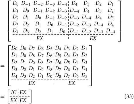
Only the top portion of the matrix is written out because they are related to the physical target domain of the original problem in the matrix operation. When using the DC-FFT algorithm, only the first row is needed, and only the first N rows of the IFFT results are the needed solutions while the others should be discarded.

IC wrap around order and pressure zero padding, shown in Figure 3, are two important operations for the DC-FFT algorithm to utilize the cyclic convolution and solve contact mechanics problems. Different implementation variations can be made; however, these two operations are necessary. The wrap-around order for deformation calculation can be done by shifting the negative side or flip those between 1~N-1. Caution should be paid for stress analyses because the shear-stress ICs are anti-symmetric. Sometimes, ICs also need zero padding, which should be done at node N where the IC is the smallest.

FIGURE 3

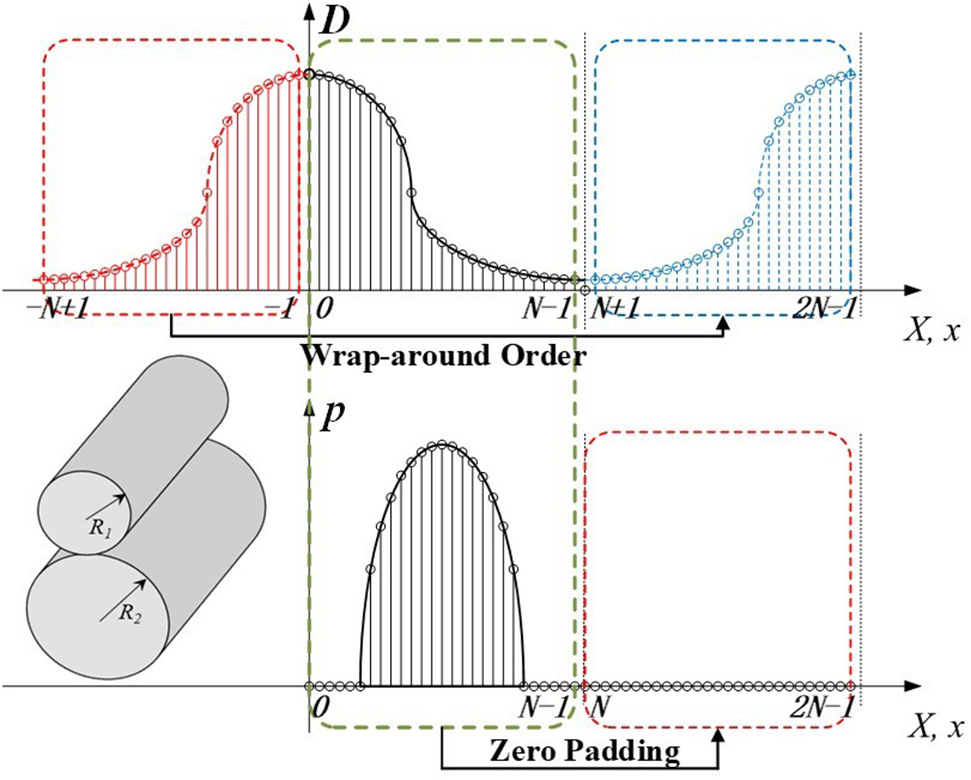
Figure 3. 1D IC wrap around order and pressure zero padding for 2D line-contact problems.

Analogous to the line-contact problem discussed above, the IC matrix for a 3D point-contact problem can be constructed by extending the original physical domain in the two lateral directions, as shown in Figure 4A. Equation (9) becomes the following for a 3D contact problem, where a is a reference length, which could be the Hertzian radius of a spherical contact, and p_h a reference pressure, which could be the maximum Hertzian pressure.

$\begin{array}{l}U=\frac{-u_z(X_k,X_l)}{a{p}_{h}C}\iff {\left[<D>\right]}_{(2N_x)(2N_y)}*{\left[P\right]}_{(2N_x)(2N_y)}\\ =IFFT\left({\left[<\widehat{D}>\right]}_{(2N_x)(2N_y)}{\left[\widehat{P}\right]}_{(2N_x)(2N_y)}\right)& (34)\end{array}$

where N_px = N_dx = N_x and N_py = N_dy = N_y are the numbers of nodes in the x and y directions, respectively.

FIGURE 4

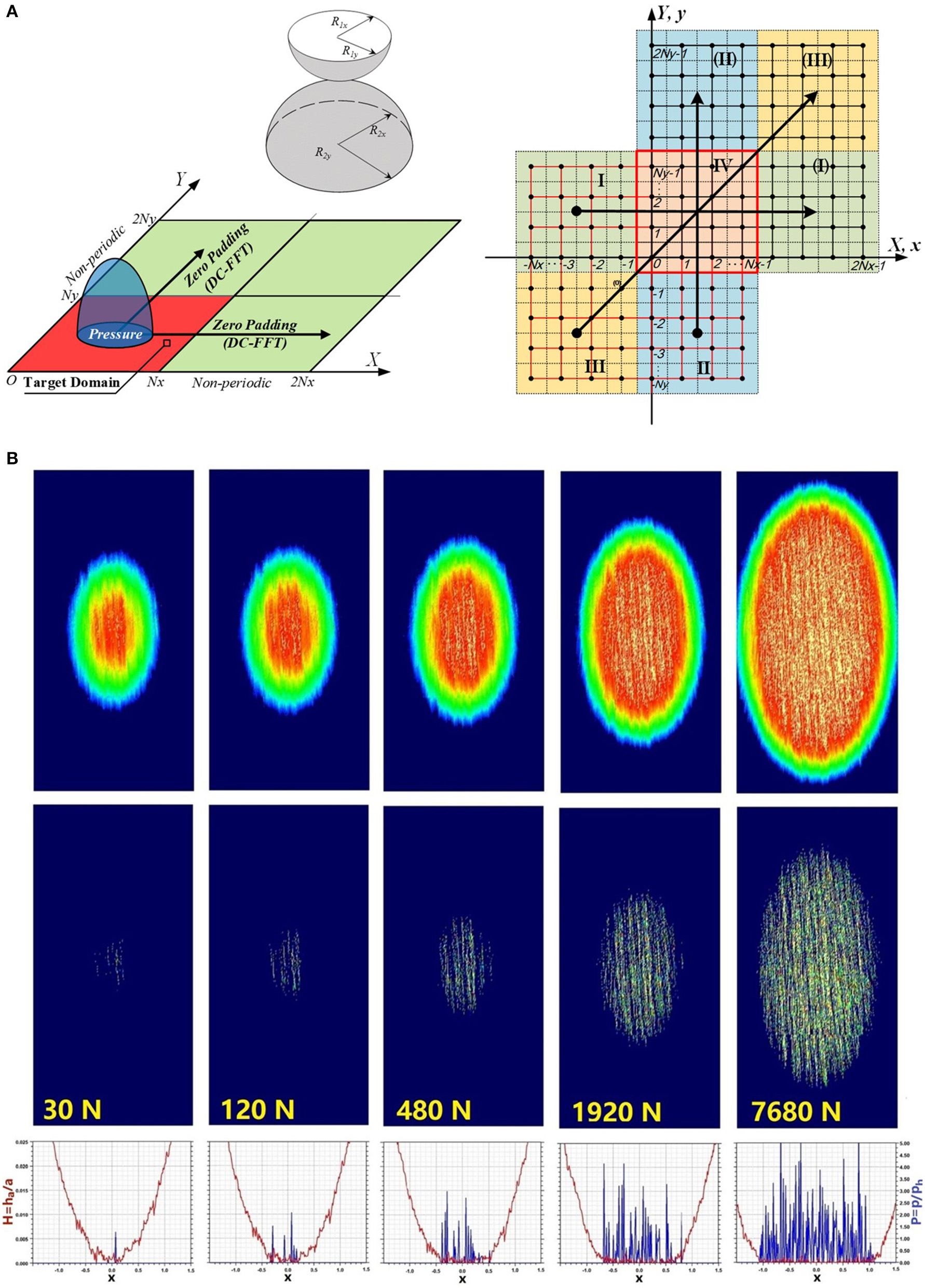
Figure 4. 2D Wrap-around order in both x and y directions and zero padding for 3D point-contact problems (A), and elliptical contacts of two rough surfaces under different normal loads (B). In (A), the arrows show the directions of the IC wrap-around order. In (B), the light-colored patterns inside the blue (middle) and red (top) contours show asperity contact pressure and area.

The extended circular convolution IC matrix is

$\begin{array}{ll}{\left[<D>\right]}_{\left(2N_x\right)\left(2N_y\right)}={\left[\langle \frac{D}{EX}|\frac{EX}{EX}\rangle \right]}_{(2N_x)(2N_y)}& (35)\end{array}$

where D on the right-hand side means the ICs corresponding to the physical domain.

It should be emphasized that two domains are involved, which are (1) the target domain, or the physical domain where the contact problem is defined, and (2) the extended domain, or the computation domain. At the end of the calculation, only the data for the target domain should be retained for the results. It is worth mentioning that the total lengths of P and D here are the minimum requirements; longer series than these should work, simply at a higher cost of computational efficiency. With these in mind, we can construct certain variations to implement this extension in order to apply the circular convolution for different situations, which are not discussed here.

The solution process involves IC matrix calculation, IC wrap-around order, pressure zero padding, and the FFT–IFFT. Its procedure is detailed as follow (Liu et al., 2000).

1) Calculate the influence coefficient matrix, [D]_2Nx×2Ny, from –N_x to N_x − 1 in the x direction and –N_y to N_y − 1 in the y direction;

2) Apply the wrap-around order and zero padding to convert the IC matrix into a cyclic matrix, [< D >]_2Nx×2Nyin the calculation domain, marked as [1 : 2Nx, 1 : 2Ny] (or [0 : 2Nx − 1, 0 : 2Ny − 1]), in the x and y directions, as shown in Figure 4B, and then apply the two-dimensional FFT to obtain the Fourier transformed IC matrix, $\left[<\hat{\hat{D}}>\right]$;

3) Input pressure, conduct zero padding to convert pressure [P]_Nx×Ny into[P]_2Nx×2Ny and then apply the two-dimensional FFT to get $\left[<\hat{\hat{P}}>\right]$;

4) Obtain a temporary frequency series using element-by-element product of the two, i.e., $\left[<\hat{\hat{D}}>\right]◦\left[<\hat{\hat{P}}>\right]$, where “◦” means the operation of element complex multiplication;

5) Conduct two-dimensional $IFFT\left(\left[<\hat{\hat{D}}>\right]◦\left[<\hat{\hat{P}}>\right]\right)$ to obtain the surface deformation and keep the result data within the original physical domain.

The error analyses by Liu et al. (2000) and Wang et al. (2003) have convinced that (1) the DC-FFT algorithm generates no additional inaccuracy beyond the discretization error, (2) its accuracy for solving elastic contact problems is nearly independent of the computation domain size accept for the necessary extension, and (3) the DC-FFT algorithm is the fastest among the commonly used contact analysis methods. Figure 4B presents a series of calculation results for the contacts of two honed rough surfaces subjected to several normal loads. The composite root-mean square (RMS) roughness is R_q = 0.5 micron. The contact ellipticity is K = 2.0, radii of curvature of the contact bodies are R_x = 19.05 mm, R_y = 54.165 mm, the equivalent elastic modulus is E′ = 226.4 GPa, and the maximum Hertzian pressure is 2.72 GPa at the load of 7,680 N. No plasticity is considered in this set of analyses. The complementary conditions for contact modeling are given in the Appendix.

Continuous Convolution and Fourier Transform (CC-FT) for Nominally Flat-Flat Contact Problems

The contact of nominally flat but rough surfaces is a problem with an infinite domain, and it can also be considered as a periodic contact problem, i.e., the contact characteristics in a representative finite region repeat periodically in lateral directions. Since the FRF of Green's function exists and the periodic pressure distribution can be made into Fourier series, the continuous convolution theorem is applicable.

The continuous convolution and Fourier transform (CC-FT) algorithm has been suggested by Liu et al. (2000) and Liu S. et al. (2007) for this type of problems, which is so named because in the theoretical nature, the continuous convolution theorem is applied. If the FT in Equation (21) and the final IFT are replaced by the discrete Fourier transform and the inverse discrete Fourier transform (IDFT), which is actually that the FT divided by mesh interval is replaced by the DFT and the IFT multiplied by the mesh interval is replaced by the IDFT, the equation below can be executed directly. Here, the FFT and IFFT are applicable to execute the DFT and IDFT efficiently. The CC-FT algorithm is built upon the frequency response functions (FRFs) $\tilde{G}$ and FFT of pressure, $\widehat{p}$,

$\begin{array}{ll}U=IDFT[\tilde{G}◦\widehat{p}]& (36)\end{array}$

The FRFs are singular at the coordinate origin, which can be processed with the Gauss quadrature integration method. This CC-FT method is actually what Ju and Farris (1996) and others used before 2000 for non-periodic contact problems where it involved periodic errors. With the CC-FT algorithm, the solution can be computed only in a representative target domain as if this were one period of the rough surface laterally. Therefore, this method is highly efficient, as well as accurate, in computation.

FFT Algorithms for 3D Line-Contact Problems

The 3D line-contact problems involve a limited domain size in one of the lateral directions but a significantly long length in the other. Such a problem can be simplified as a 2D plane-strain issue if the contacting surfaces are ideally smooth and the materials homogeneous. To explore more detail, we are facing 3D problem with mixed issues. Three FFT-based approaches have been developed, to be discussed below, which are the algorithms of mixed discrete-continuous convolution with duplicated padding and FFT (DCD-FFT) (Chen et al., 2008), the hybrid discrete convolution, continuous convolution and FFT (DC-CC-FFT) (Liu and Hua, 2009), and the discrete-periodic convolution with IC summation and FFT (DCS-FFT) (Liu and Hua, 2009; Sun et al., 2020) to consider the effect of roughness and material inhomogeneity. They are mathematically and numerically the same in the finite direction (x), but different in the other dimension (y).

DCD-FFT Algorithm

The DCD-FFT algorithm (Figure 5A) modifies the DC-FFT algorithm with a treatment in the y direction, simply by duplicating the pressures in the target domain to the extended region in the y direction, called duplicated padding (Chen et al., 2008). The length of the extended region should be at least the same as that of the target domain. This method is not as accurate as the DC-FFT one for non-periodic problems, especially when the extended domain in y is not sufficiently long, because it ignores the deformation influences from the region not included in the calculation, and the IC truncation error plays a role. Therefore, this method is mentioned here for a reference use only. However, the DCD-FFT method can effectively solve the normal deformation of finite-cylinder surfaces (a quarter-space problem), if the cylinders are not too short, with pressure duplication in the extended domain (Liu et al., 2020).

FIGURE 5

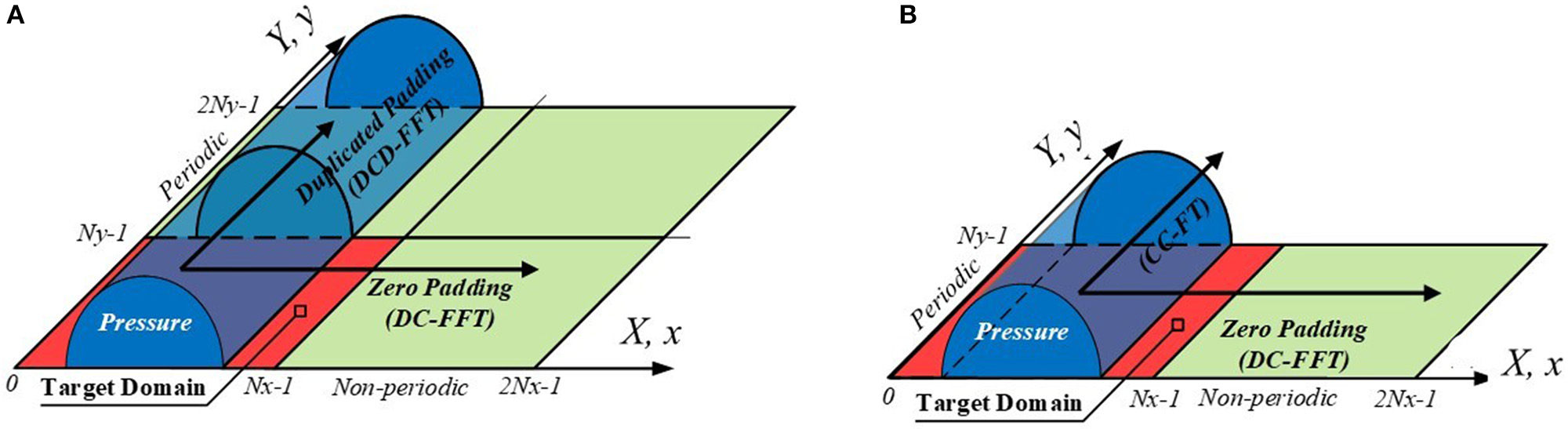
Figure 5. DCD-FFT (A) and DC-CC-FFT (B) algorithms (based on Sun et al., 2020), Reprinted by permission from Springer, Computational Mechanics. The red areas mark the target domains, and the light green regions are for the IC wrap around.

DC-CC-FFT Algorithm

The infinite extension of the problem in the y direction qualifies the direct use of the CC-FT method. Thus, the DC-CC-FFT algorithm combines the features of the discrete convolution theorem in the x direction, and the continuous convolution theorem in the y direction, shown in Figure 5B, involving hybrid FRFs and ICs (named ICs-FRF). Because there are two ways to obtain the FRFs for the y-direction solution, two variations of the DC-CC-FFT algorithm can be constructed.

DC-CC-FFT with IC-conversion. A simple way, with known ICs, described by Sun et al. (2020), to build the DC-CC-FFT algorithm is to process the 2D Fourier transform of the ICs sequentially in the y and the x directions to obtain ICs-FRF, where the FRF is from the IC conversion. After the y-direction FFT, the FRFs are calculated from Equations (14) and (17). Then the wrap-around order in the x direction is conducted, followed by the 1D Fourier transform in x. The calculation can be performed in the following steps with a slightly different procedure for the wrap around order.

1) Input the pressure, [P]_{Nx× Ny};

2) Extend the pressure [P]_Nx×Ny into [P]_2Nx×Ny with zero-padding in the x direction only;

3) Transform [P]_2Nx×Ny to ${\left[<\widehat{\widehat{P}}>\right]}_{2N_x\times N_y}$by applying 2D FFT, note here, the domain has been enlarged;

4) Calculate the IC matrix [D]_{2Nx× Ny};

5) Apply 1D FFT to [D]_2Nx×Ny in the y direction to get ${\left[\widehat{D}\right]}_{2N_x\times N_y}$;

6) Calculate the ICs-FRF, ${\left[\tilde{D}\right]}_{2N_x\times N_y}$ by using Equations (14) and (17) in the y direction;

7) Treat ${\left[\tilde{D}\right]}_{2N_x\times N_y}$with the wrap-around order only in the x direction and get ${\left[<\tilde{D}>\right]}_{2N_x\times N_y}$ which is only term flip because the domain has been enlarged in 4). Here, ${\left[<\tilde{D}>\right]}_{2N_x\times N_y}$ is the ICs after the wrap around order in the x direction but FRF in the y direction, and the latter is converted from the ICs done in the previous step;

8) Apply 1D FFT to ${\left[<\tilde{D}>\right]}_{2N_x\times N_y}$ in the x direction, and the resultant series is denoted as ${\left[<\widehat{\tilde{D}}>\right]}_{2N_x\times N_y}$;

9) Obtain a temporary frequency series by element-by-element production between ${\left[<\hat{\hat{P}}>\right]}_{2N_x\times N_y}$ and ${\left[<\widehat{\tilde{D}}>\right]}_{2N_x\times N_y}$, which can be expressed as $\left[<\widehat{\tilde{D}}>\right]◦\left[<\hat{\hat{P}}>\right]$, where “◦” means complex multiplication in an element-by-element manner;

10) Apply a 2D IFFT to $\left[<\widehat{\tilde{D}}>\right]◦\left[<\hat{\hat{P}}>\right]$;

11) Obtain the surface displacement by keeping values within the original target domain, and the resultant series are shown as $IFFT\left\{\left[<\widehat{\tilde{D}}>\right]◦\left[<\hat{\hat{P}}>\right]\right\}$.

The advantage of the algorithm of DC-CC-FFT with IC-conversion is that it does not require known FRFs if ICs can be calculated more easily. It is more accurate than the DCD-FFT method but still involves some IC truncation and conversion errors. The IC truncation error can be greatly reduced by using the IC summation method, to be discussed in section DCS-FFT Algorithm.

Precise DC-CC-FFT algorithm, presented by Liu and Hua (2009), is to conduct the analytical Fourier transform of Green's function in the length (y) direction, and calculate the ICs with respect to x, to obtain the hybrid ICs-FRFs, and then conduct the wrap-around order in x and the one-dimensional FFT of the new ICs-FRFs. This approach is theoretically accurate.

Both DC-CC-FFT algorithms only require extending the domain in the x direction twice the size of the target domain, while the domain size in y is unchanged, which can be as small as possible, as long as it is sufficient represent the necessary features of surfaces and materials.

DCS-FFT Algorithm

Liu and Hua (2009) suggested another approach to deal with 3D line-contact problems, which is to consider the elasticity effect of the entire domain, or a sufficiently large domain, by IC summation, and Sun et al. (2020) have extended this method to solve the contact problems involving inhomogeneous materials. Figure 6A illustrates this idea. We can include M segments of equal length on each side of the target domain in the length direction, while making the target domain size as small as possible, as long as the main contact features are included. N_x in the x direction and N_y in the y direction may be different.

FIGURE 6

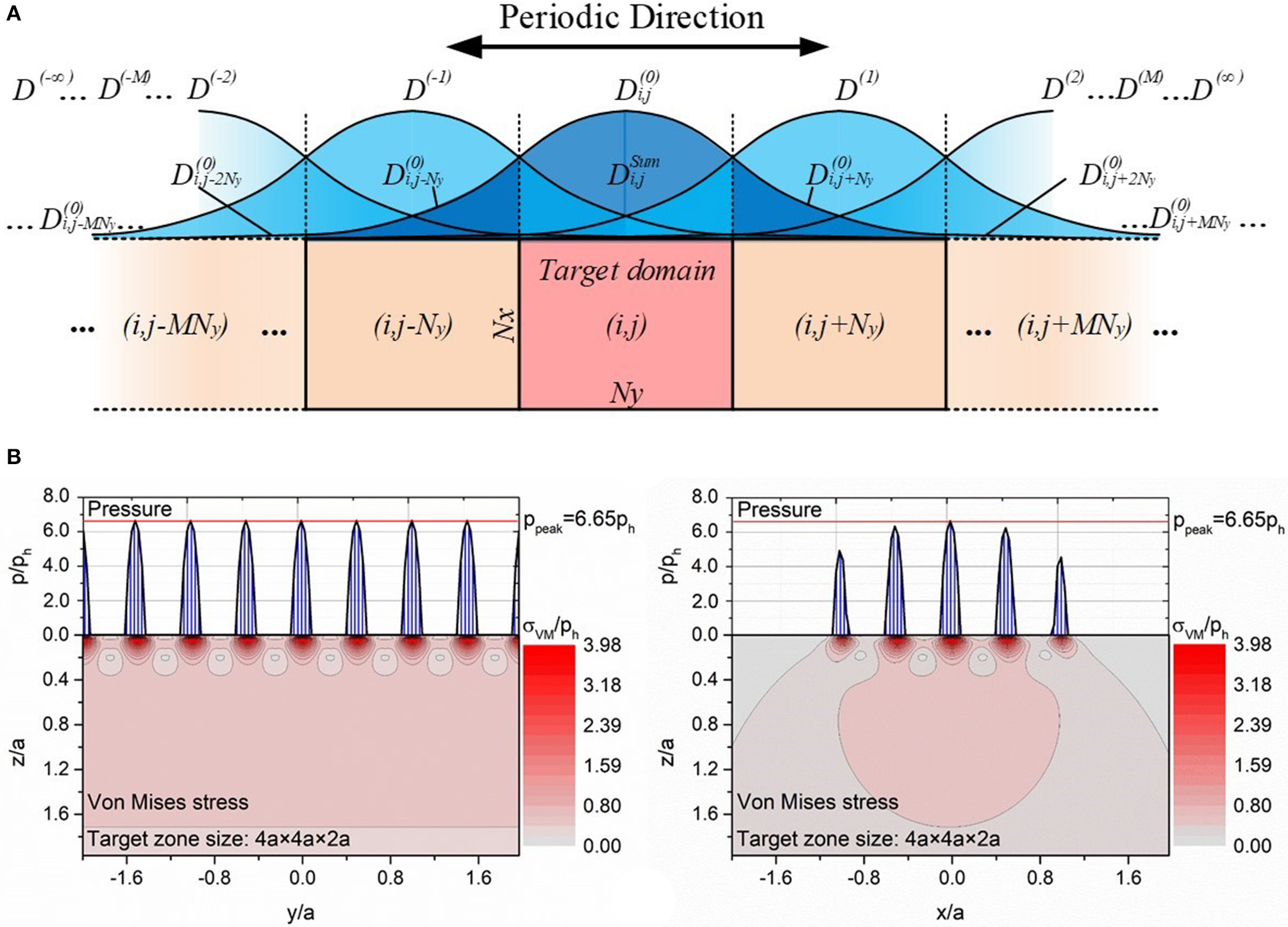
Figure 6. IC summation in the periodic convolution (A) and 3D line contact of a smooth, rigid cylinder, and a flat rough surface calculated by using the DCS-FFT algorithm (B).

The ICs in each segment are the same, periodically shifted from those in the target domain. The influences of the pressures in the other segments on the deformation within the target domain can be included via the IC summation in the target domain, given below, with the superscripts for the segment numbers and the subscripts for the y direction coordinates in the target domain.

$\begin{array}{ll}{D}_{i,j}^{Sum}={\displaystyle \sum _{r=-M}^M}\left(D_{i,j-r{N}_y}^{(r)}\right),0\le i\le N_x-1,0\le j\le N_y-1& (37)\end{array}$

Because the ICs in each segment are the same, only one copy of the IC, marked with superscript (0), is necessary, shown below with proper shifts for other copies.

$\begin{array}{ll}{D}_{i,j}^{Sum}={\displaystyle \sum _{r=-M}^M}\left(D_{i,j-r{N}_y}^{(0)}\right),0\le i\le N_x-1,0\le j\le N_y-1& (38)\end{array}$

Using $D_{i,j}^{Sum}$ in the DC-FFT algorithm should result in more accurate solutions to 3D line-contact problems than those by using the DCD-FFT algorithm. Of course $D_{i,j}^{Sum}$ can be used in the algorithm of DC-CC-FFT with IC-conversion discussed in the previous section. The solution procedure of the DCS-FFT algorithm can utilize the DC-FFT framework, which may involve the following steps:

1) Calculate the summed IC matrix, $D_{i,j}^{Sum}$, from the ICs calculated in the region from –N_x to N_x-1 in the x direction and from −MN_y to MN_y-1 in the y direction, and construct ${\left[D\right]}_{N_x\times N_y}^{Sum}$

2) Apply the wrap-around order, as well as zero padding if needed, to transfer the IC matrix into a cyclic matrix, ${\left[<D>\right]}_{2N_x\times 2N_y}^{Sum}$, similar to that in the DC-FFT algorithm, and then employ the 2D FFT to obtain the Fourier transformed IC matrix, ${\left[<\widehat{\widehat{D}}>\right]}^{sum};$;

3) Input pressure, conduct zero padding in the x direction and duplicated padding in the y direction to convert pressure [P]_Nx×Ny into [P]_2Nx×2Ny, and apply the 2D FFT to get the Fourier transformed pressure matrix, $\left[<\hat{\hat{P}}>\right]$;

4) Obtain a temporary frequency series from the element-by-element complex product of the two, as ${\left[<\hat{\hat{D}}>\right]}^{Sum}◦\left[<\hat{\hat{P}}>\right]$;

5) Obtain the surface deformation data from $IFFT\left\{{\left[<\hat{\hat{D}}>\right]}^{Sum}◦\left[<\hat{\hat{P}}>\right]\right\}$ and keep the resultant data within the original physical target domain.

Figure 6B presents the 3D cylindrical contact of a rigid infinite-length cylinder and an elastic half space material (E = 200 GPa, υ = 0.3) with a sinusoidal rough surface, analyzed with the DCS-FFT algorithm. The 3D roughness is periodic in both the x and y directions, and the load is treated periodically in the y direction. With the DCS-FFT method, no edge effect appears at the borders of the target domain, which means that the elasticity effect of neighboring duplicated domains has been properly taken into account.

Compared with the DCD-FFT algorithm, the DCS-FFT method does not require a large target domain because of the IC summation. As mentioned before, N_y can be very small, e.g., as small as one period of the pressure variation in the y direction, or as short as the length of a representative rough surface area and/or material inhomogeneity region. Among all the three algorithms for 3D line-contact problems, the DCS-FFT and the accurate DC-CC-FFT algorithms are recommended, and the former may be more preferred because it uses the same DC-FFT solution framework, convenient for programming, especially when the DC-FFT software is available as a set of the open-source codes (http://othello.mech.northwestern.edu/qwang/OpenSourceCodeDCFFT/DC-FFTWeb.htm). It should be mentioned that the DCS-FFT algorithm can also be used to construct a mechanism to solve the nominally flat-flat contact problems, named DCSS-FFT, which further modifies the ICs with 2D IC summations in both x and y directions (Sun, 2020).

DCR-FFT Algorithm

In comparison to the contact issues involving an excitation and response defined in a convolution, the relationship between eigenstrains and the components of the elastic field in a material involves both the convolution and the correlation (Liu and Wang, 2005; Liu et al., 2012), and the correlation theorem should be implemented as well. Here, eigenstrain is a generic term for various non-elastic strains, defined by Mura (1993), including thermal strain, plastic strain, fit-induced strain, phase transformation induced strain, and residual strain in a general sense. Many inhomogeneity problems can be solved via the Equivalent-eigenstrain method (EIM) (Eshelby, 1957), and correlations of functions are involved in the mathematical expressions of the eigenstrain-induced field.

Correlation Theorem

The Fourier transform of the correlation of two real datum series is the multiplication of the complex conjugate of Fourier transform of one function and the Fourier transform of the other.

$\begin{array}{ll}\text{Correlation }{\displaystyle \underset{-\infty }{\overset{\infty }{\int }}}g(t+\tau )f(t)dt=R_{Gf}(\tau )& (39)\end{array}$

with _{RGf(τ) = RfG(−τ)}, and the Fourier transform is,

$\begin{array}{ll}{\tilde{R}}_{Gf}(m)=\tilde{g}(m)\overline{\tilde{f}(m)}& (40)\end{array}$

where $\overline{\tilde{f}}$ is the complex conjugate of $\tilde{f}$.

DCR-FFT Algorithm

The DCR-FFT algorithm is an analogy to the DC-FFT algorithm, to be proven below, and it can be combined with the DC-FFT algorithm for a hybrid convolution-correlation operation to solve the inhomogeneity problem illustrated in Figure 1D. Details are given by Liu and Wang (2005), and applications can be found in the works by Liu et al. (2012), Wang et al. (2013a,b), Zhou et al. (2016), and Zhang M. Q. et al. (2018). A set of open-source codes can be downloaded from http://othello.mech.northwestern.edu/qwang/OpenSourceCodeEigenstrainFiledHalfSpace/2012Web.htm.

Let's use deformation as an example. Equation (41) (Liu et al., 2012) shows the link between eigenstrain [e] in domain Ω and surface deformation u_i in the i = x, y, or z direction, via a group of Green's functions, ${\text{U}}_i^s$.

$\begin{array}{ll}{u}_i=\frac{-1}{2\pi }{\displaystyle {\int }_{\Omega }{\text{U}}_i^s[e]d{\text{x}}^{\prime }}& (41)\end{array}$

Similar to the expression of convolution related to potential function $R^I=\sqrt{{\left(x-\xi \right)}^2+{\left(y-\eta \right)}^2}$ for the solution to contact elasticity, Equation (41) involves $R^I=\sqrt{{(x-\xi )}^2+{(y-\eta )}^2+{(z-\zeta )}^2}$ and $R=\sqrt{{\left(x-\xi \right)}^2+{\left(y-\eta \right)}^2+{\left(z+\zeta \right)}^2}.$ Here, R has a plus sign inside the third term, which means a 1D cross correlation with [e] on z for the solution.

The discrete form of the 1D cross correlation of influence coefficient D and [e] in Equation (41) is given below

$\begin{array}{ll}{u}_z={\displaystyle \sum _{i=1}^{N_e}{D}_{i+k}{e}_i}& (42)\end{array}$

where N_e is the total number of nodes, and IC components D_k+i involves R.

More generally, for two series of complex numbers, f and g,

$\begin{array}{ll}{R}_{hg}={\displaystyle {\int }_{-\infty }^{\infty }}\overline{f(t)}g(t+\tau )dt& (43)\end{array}$

where $\overline{f(t)}$ is the complex conjugate of f(t). Equation (42) is equivalent to the following correlation,

$\begin{array}{ll}{R}_{hg}={\displaystyle {\int }_{-\infty }^{\infty }}\overline{f(t-\tau )}g(t)dt\text{ and }{\tilde{R}}_{hg}=\overline{\tilde{f}(t-\tau )}\tilde{g}(t)& (44)\end{array}$

$\begin{array}{ll}\text{Or }{R_{hg}}_{\left[n\right]}\equiv {\displaystyle \sum _{m=-\infty }^{\infty }}\overline{f_{\left[m-n\right]}}{g}_{\left[m\right]}\text{ and }{\widehat{R}}_{hg}=\overline{\widehat{f}(t-\tau )}ĝ(t)& (\mathrm{44’})\end{array}$

This means that the convolution theorems should also be true to Equation (44) or (44’), no matter the series are real or complex. The numerical calculation of correlation can be done either by direct use of the correlation theorem (Equations 39–40) or the convolution given in Equation (44) (or Equation 44’) with proper treatment of the two series, and the DC-FFT algorithm directly works for the latter. Caution should be given in conducting the Fourier transform.

By analogy, the DC-CC-FFT and CC-FT algorithms can all be extended to include the correlation operation for the analyses of the field due to eigenstrains.

Figure 7 shows a case of a cylinder in contact with the rough surface of an inhomogeneous half-space material (Sun et al., 2020), solved with the DCS-FFT algorithm. The representative piece of a ground surface is given in Figure 7A) in a mesh of 128 × 128, and R_q= 1.18μm. A virtual ground rough surface subjected to the cylindrical contact is formed through periodically extending this patch along the y direction. The target domain has the dimensions of l_x×l_y×l_z, and the length are all set to be $l_x=l_y=\frac{8a}{3}$, $l_z=\frac{4a}{3}$. All the cuboidal inhomogeneities are identical, with a_x = a_y = a_z = 0.3a, and they are distributed in the subsurface in the x = 0 plane in the depth of z_d = 0.45a. Figure 7B shows the 3D pressure distribution mapped on the contact surface, where sporadic pressure peaks can be found. The contours of the pressure and the von Mises stress distributions in the XOZ and YOZYOZ cross sections are given in Figures 7C,D. The 3D features of the pressure and stress are captured while their length-direction periodicities are also retained.

FIGURE 7

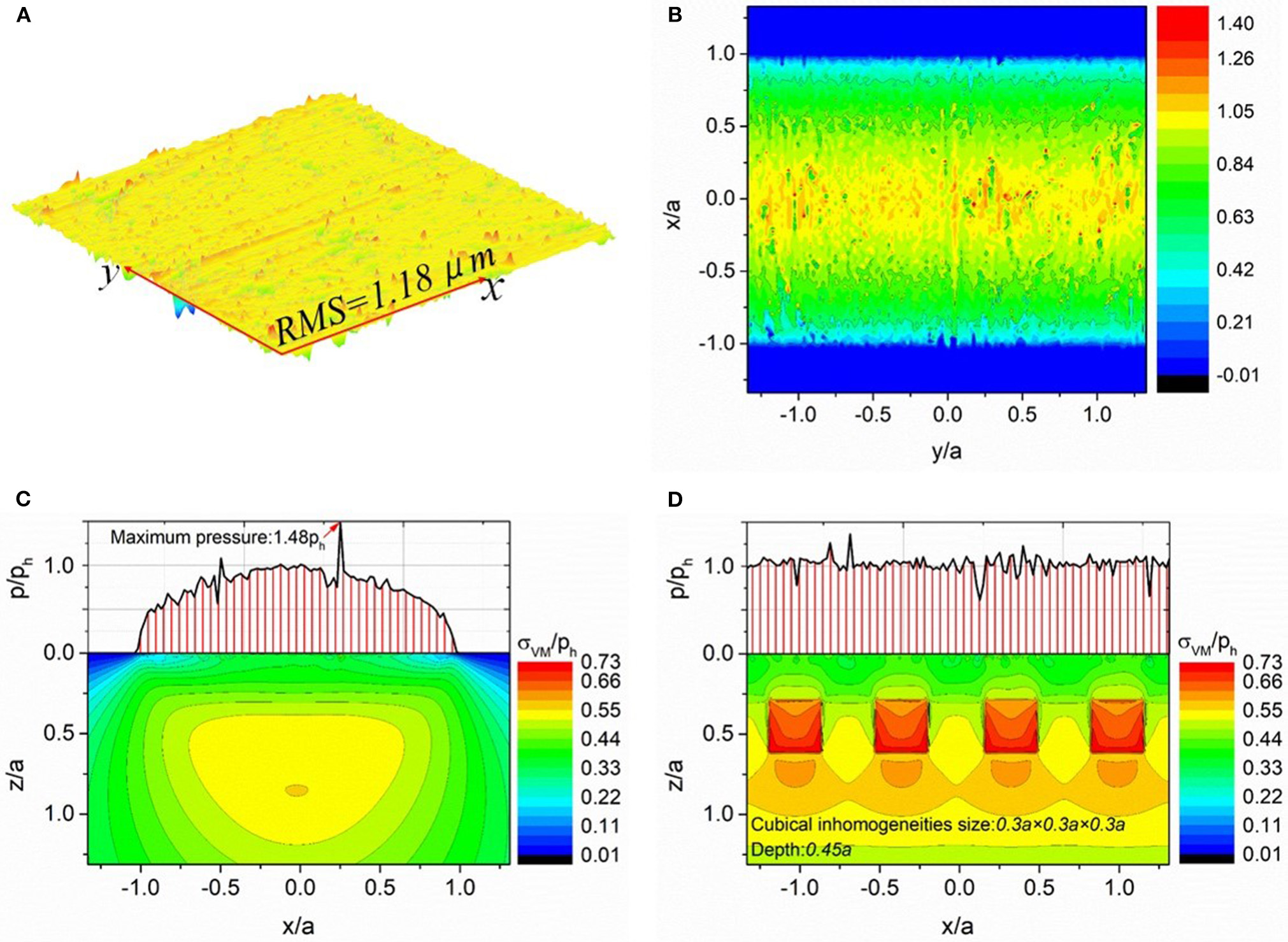
Figure 7. Contact of a cylinder with inhomogeneous half-space and a rough surface (A) and inhomogeneities, 3D pressure distribution on the contact surface (B), pressure and von Mises stress distributions in the XOZ plane (C), and pressure and von Mises stress distribution in the YOZ plane (D). The square inhomogeneities are shown in (D). Note that (C) cuts through the center of the domain, where no inhomogeneity appears.

IC Conversion From FRFs

Figure 1E shows the contact involving a multi-layered material. The core analytical solutions to this type of problems are obtained, ignoring the body forces, by solving the governing differential equations in the frequency domain through the Fourier transform. The Fourier-domain solutions become the frequency response functions (FRFs) if surface tractions are unit valued. The conversion through Equations (13)–(18) leads to influence coefficients for the DC-FFT algorithm (Liu and Wang, 2002; Yu et al., 2014, 2016). Note that here, the direct inverse Fourier transform of the frequency-domain solution may result in inaccuracy when solving a non-periodic non-infinite contact problem (Liu et al., 2000).

The IC conversion method can be used to other contact cases as well. Our recent studies on the contacts involving magnetoelectroelastic or viscoelastic materials are all through the path of FRFs-ICs conversion and then the DC-FFT algorithm. Two such examples are given in Figures 8, 9.

FIGURE 8

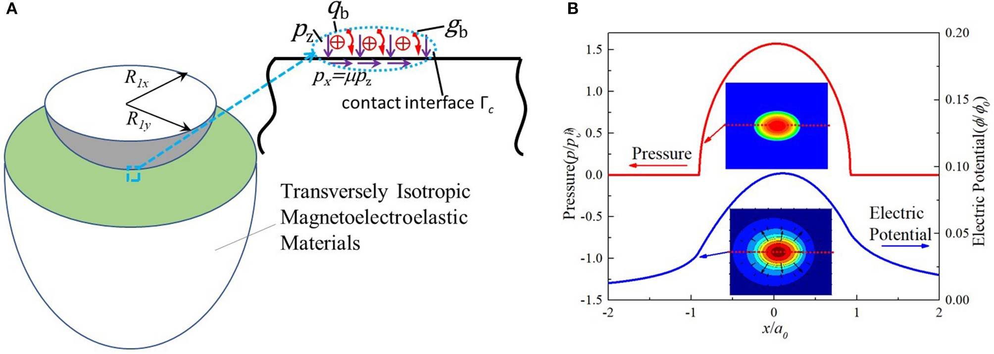
Figure 8. Contact of magnetoelectroelastic materials subjected to interfacial contact pressure, p_z, friction, p_x, surface electric and magnetic charges, q_b and g_b, (A); solutions of pressure and electrical potential on the surface (B).

FIGURE 9

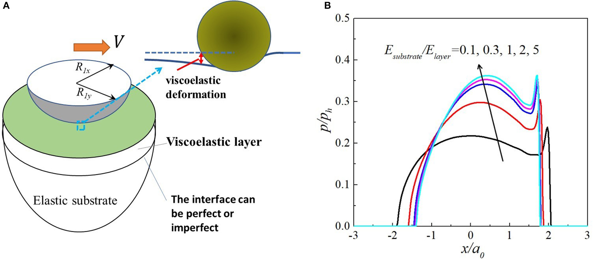
Figure 9. Sliding contact of a viscoelastic layer-elastic substrate system (A); and the pressure variations in the case of a sphere sliding on the surface of such a material set at speed V = 50 mm/s (B). This model includes four cases, (1) a viscoelastic layer on an elastic substrate, as shown, (2) a viscoelastic half space, layer thickness = ∞, (3) an elastic half space, layer thickness = 0, and (4) an elastic layer on a viscoelastic substrate by exchanging material properties under certain conditions.

Figure 8A shows the contact of two magnetoelectroelastic materials subjected to interfacial contact pressure, surface electric and magnetic charges. For this type of multifield material systems, the Fourier-domain solutions can be obtained by solving the coupled mechanical governing equations and the Maxwell equations in the frequency domain through the Fourier transform. The Fourier-domain solutions become the FRFs if the mechanical tractions, surface electric and magnetic charges are unit valued. The inverse Fourier transform through Equations (13) and (18) leads to influence coefficients to construct the DC-FFT algorithm. Figure 8B shows a case of an ellipsoid in contact with the surface of a magnetoelectroelastic material. The major and minor radii of the ellipsoid are R_x = 300 mm and R_y = 200 mm, and the normal force is P_z = 500 N. More details can be found in the work by Zhang X. et al. (2017, 2018, 2019).

Viscoelastic contact problems have drawn a great deal of attention (Goryacheva and Sadeghi, 1995; Chen et al., 2011; Putignano et al., 2015; Stepanov and Torskaya, 2018). It is also convenient to solve certain viscoelastic contact problems in the frequency domain. Here, two types of frequencies are involved, one with respect to time and the other to space. Figure 9A shows the sliding contact of a layer- substrate system, which actually represents four cases for each contacting bodies, (1) a viscoelastic layer on an elastic substrate, as shown, (2) a viscoelastic half space with the layer thickness = ∞, (3) an elastic half space with the layer thickness = 0, and 4) an elastic layer on a viscoelastic substrate by exchanging material properties under certain conditions, all solvable with the same model (Zhang et al., 2020a,b). The FRFs can be readily obtained from the elastic FRFs of elastic layered materials, by replacing the elastic modulus in elastic FRFs with the viscoelastic complex modulus. The inverse Fourier transform of the viscoelastic FRFs through Equations (13) and (18) leads to the viscoelastic influence coefficients to construct the DC-FFT algorithm in the viscoelastic contact framework. Figure 9B shows a case of a sphere sliding on the surface of a viscoelastic layer-elastic substrate system at a contact speed V = 50 mm/s. The layer thickness is 1 mm, the sphere radius is 10 mm, and the normal load is 1.48 N. Note that in Figure 9A, the interface between the layer and the substrate can be imperfect, and the spatial domain ICs have been solved by Wang et al. (2017a,b) and Zhang and Wang (2020). More studies related to viscoelastic contact solutions of layered materials with perfect or imperfect interfaces subjected to steady-state and transient conditions can be found in the work by Zhang et al. (2020a,b).

FFT With Non-uniform Mesh

In engineering systems, such as gears, journal bearings, and manufacturing tools, the contact regions can be large but the computation scale in a numerical simulation is limited. It is always a challenge to balance efficiency and accuracy. Take the line contact in a gear or a roller bearing as an example; the middle portion of the contact zone can be analyzed accurately with a coarse mesh, but the edges have to be modeled with a fine mesh in order to describe the drastic pressure variations there. The FEM deals with this type of issues with non-uniform meshes; however, the FFT-based methods built so far, although efficient in a single mesh, are largely confined by the requirement of uniform grids. Sun (2020) has developed a method to extend the FFT-based algorithms to meshes of different densities, in which a finer mesh system is used in specific regions involving high pressure peaks while a coarser one is set in other regions under relatively smooth pressures. Figure 10A illustrates this non-uniform-mesh idea for a roller contact problem, where one side of the regions under the edge effects is meshed denser, while the other side is meshed with a coarse grid. In this particular example, the density of the fine grid is three times that of the coarse grid. The solution on the coarse-grid domain may be run for the entire region, depending on the size of the problem, but that on the fine-mesh domain is pursued just in a region somewhat larger than what it is designated. Extra data are discarded, and the joint deformations from the two meshes in both designated regions are used to evaluate the gap. This process involves overlapped calculations; however, for problems like the roller contact shown here, the larger the physical domain is, the more the saving of the computation time.

FIGURE 10

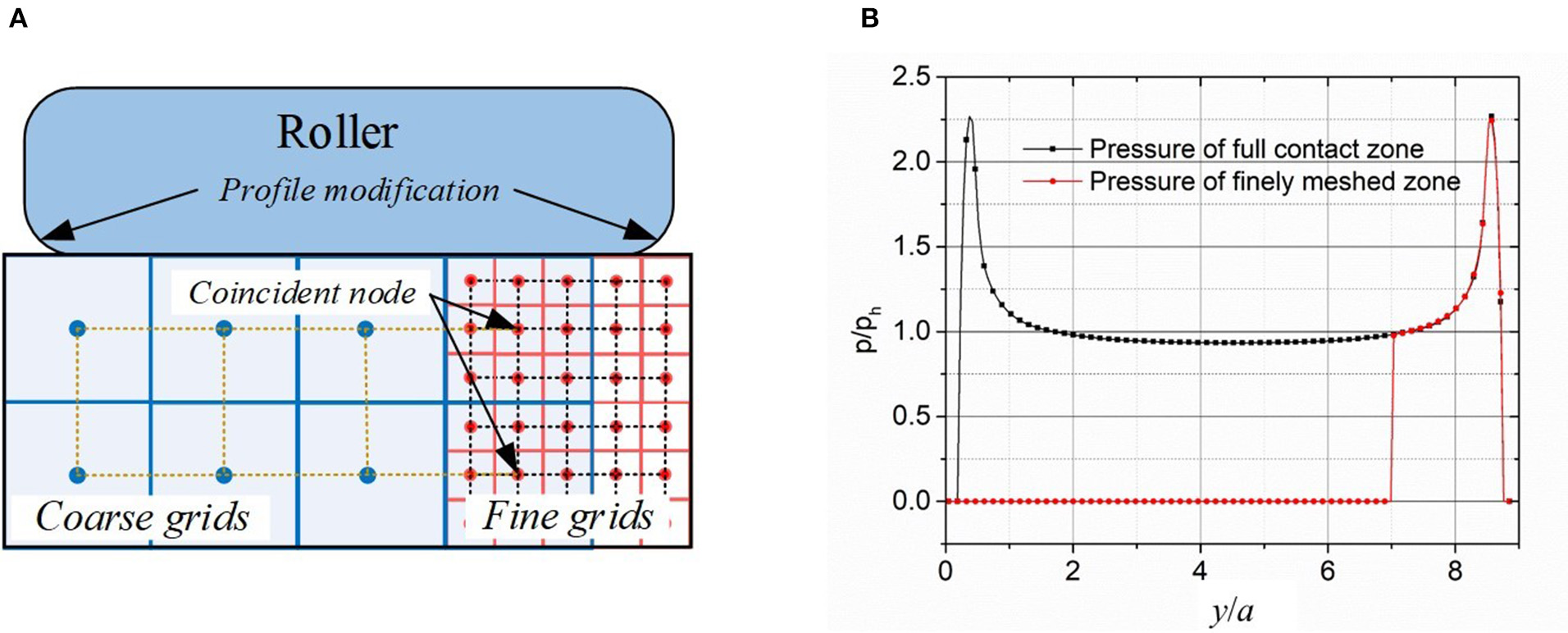
Figure 10. Non-uniform mesh system used in the contact of a bearing roller with an end profile modification (A), and a calculation result (B).

Figure 10B shows the comparison of the pressure calculated with a uniform mesh system and non-uniform meshes. The density of the uniform mesh is the same as that of the fine mesh of the non-uniform meshes. The pressure obtained on the effective zone of the fine mesh from the non-uniform mesh solution well matches that on the uniform fine mesh system. When the contact region is large and the pressure distribution is strongly non-uniform, the FFT method with non-uniform meshes offers a more efficient and flexible way to detail the regions of special concerns, such as edges, interfaces, dents, and defects.

Discussion and Conclusions

Accuracy Comparisons

Figure 11A is for the results of a finite-domain problem with pressure acting on a region of 2a in length (Liu et al., 2000); it compares the errors from the DC-FFT algorithm structured in different routes with respect to the solution from the direct summation (DS) method. The continuous convolution and Fourier transform (CC-FT) algorithm is used to solve the same finite-domain problem, and its result is also compared. In this figure, the solution methods are named routes, which are Route 2: DC-FFT with ICs from Green's function, Route 3: DC-FFT with ICs from conversion of frequency response functions, Route 4: CC-FT with frequency response functions, Route 5: the classic DS method with ICs from Green's function. Route 1 is not included here, which uses the FEM to calculate the ICs. The DC-FFT solution method (Route 2) appears to be accurate; its results overlap with those by the DS method. This means that the solution is not affected by the calculation domain size. Route 3, however, is different, depending on the discretization density in the frequency domain. The discrete influence coefficient from the frequency response function is the key for error control, the frequency domain sampling intervals, Δ_m and Δ_n, should satisfy N_m≥2N_x and N_n≥2N_y, and Equations (16), or (17), or (18) should be implemented, followed by a proper wrap-around order (Liu and Wang, 2002).

FIGURE 11

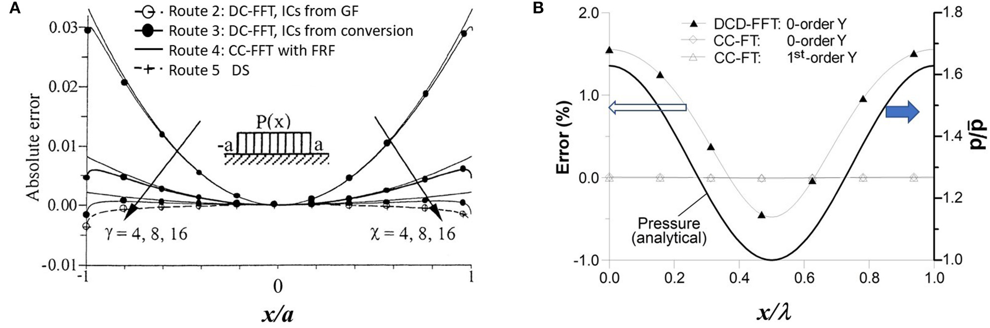
Figure 11. Error comparisons. (A) DC-FFT and CC-FT algorithms in solving a finite-domain problem (Liu et al., 2000), Reprinted by permission from Elsevier, Wear, γ means the discretization density in the frequency domain and χ the ratio for spatial calculation domain extension, (B) CC-FT and DCD-FFT algorithms in solving the contact of a 3D sinusoidal wavy surface and a flat (Liu S. et al., 2007), Reprinted by permission from Elsevier, Tribology International; this is an infinite-domain, or periodic, problem. $\overline{p}$ means the average pressure.

Figure 11B shows the behavior of the CC-FT algorithm in solving the periodic problem of a 3D sinusoidal wavy surface in contact with a flat; it compares the numerical solution with the corresponding analytical results results (Liu S. et al., 2007). In addition, the DCD-FFT algorithm is also evaluated. It is evident that the CC-FT algorithm yields the solutions of high accuracy that is within machine precision. The CC-FT algorithm with either the zero-order or the first-order shape function yields nearly the same high accuracy. This indicates that a higher order shape function may be unnecessary if the algorithm is formulated properly.

The CC-FT algorithm is superb in analyzing the contact of nominally flat but actually rough surfaces.

Figure 12 compares the 3D cylindrical-contact algorithms of DCS-FFT, DCD-FFT, and DC-CC-FFT with IC-sum-conversion in calculating the maximum shear stress τ₁, given below:

$\begin{array}{ll}{\tau }_1=\frac{1}{2}\sqrt{{({\sigma }_{11}-{\sigma }_{33})}^2+4{\sigma }_{13}^2}& (45)\end{array}$

The identical target domain (2a×2a×2a) is used in all the three FFT-based methods. A large gap is shown between the result curves for the analytical and the DCD-FFT results, caused by the IC truncation error. The utilization of the DC-CC-FFT algorithm (IC-summation-conversion) greatly reduces the truncation error; however, some difference is still visible. The advantage of this DC-CC-FFT algorithm with the summarized ICs is the reduced computational burden because no duplicated-padding and wrap-around order are needed in the length direction. The DCS-FFT algorithm shows its accuracy and efficiency in dealing with this type of contact problems without knowing analytical FRFs. Theoretically the precise DC-CC-FT algorithm is more accurate (Liu et al., 2009), which is similar to the CC-FT shown in Figure 11B.

FIGURE 12

Figure 12. Comparison of the algorithms of DCS-FFT, DCD-FFT and DC-CC-FFT with IC-sum conversion. The physical domains are marked as x × y × z, and M = 8 means the number of segments used in the IC preparation.

Range of Applications of the FFT Approaches

The FFT-based approaches are efficient. Many publications have shown the applications of these FFT algorithms on the contact analyses of elastic fields, plastic transition and yield, flash temperature, thermal stress, partial slip, and contact electrical and magnetic fields, dealing with science and mechanics issues for various systems from traditional mechanical components to emerging sensors and batteries (Zhang X. et al., 2019; Zhang et al., 2020c). The FFT algorithms discussed above are advantageous in solving the problems that are mathematically described in convolutions, correlations, combined convolutions and correlations, and in frequency response functions as well. The last one makes the FFT-based approaches more widely applicable and powerful because many governing differential equations can be more easily solved in the frequency domain through the Fourier transform, such as those for functionally graded materials (Ke and Wang, 2006), thermoelastically graded materials (Choi and Paulino, 2008), thermally graded materials (Zhang H. B. et al., 2018), materials with coupled stresses (Wang et al., 2020), and magnetoelectroelastic materials (Zhou and Lee, 2013). In addition, because the surface deformation analysis is an intermittent process of the elastohydrodynamic lubrication (EHL) calculation and related modeling, the FFT-based solutions are also building blocks in the models of mixed EHL in general (Liu et al., 2006, 2009), 3D line-contact EHL (Ren et al., 2009), finite-roller EHL (Zhang H. B. et al., 2017 with IC-overlapping DC-FFT, Liu et al., 2020 with DCD-FFT), coating EHL (Liu Y. et al., 2007 for single coatings, Wang et al. (2015) for multilayered coatings), plasto-EHL (Ren et al., 2010), EHL of inhomogeneous materials (Wang et al., 2014), wear in EHL (Zhu et al., 2007), EHL of transversely isotropic materials (Wang and Zhang, 2019), EHL of artificial joints (Wang and Jin, 2004), and EHL of 2D bearings (Liu and Chen, 2012). Moreover, adhesive contact problems can be solved with the FFT-based methods as well (Pohrt and Popov, 2015; Popov et al., 2017; Rey et al., 2017).

It is important to note that different contact types require different convolution theorems and thus different FFT algorithms. As summarized by Wang and Zhu (2019), contact with nominally flat surfaces should be tackled with the continuous convolution and Fourier transform (CC-FT) algorithm. Point-contact problems, either circular or elliptical, are non-periodic, and they should be formulated with the cyclic convolution and solved with the discrete convolution and FFT (DC-FFT) method utilizing zero padding and wrap-around order. Three-dimensional cylindrical (line) contact problems involve infinite domain extension in one direction but a finite domain width in the other, for which the discrete-continuous convolutions and FFT (DC-CC-FFT) and the discrete convolution with IC summation and FFT (DCS-FFT) methods should be used. The DCS-FFT algorithm is recommended if ICs are already known. Both the CC-FT and DCS-FFT algorithms are capable of solving periodic problems, and if the latter is used, the IC summation in the other direction is also needed, which makes it the DCSS-FFT algorithm mentioned in section DCS-FFT Algorithm. Figure 13 summarizes the FFT algorithm tree and the application field of each. The roots of this tree are the essential analytical solutions to mechanics and physical problems in the forms of Green's functions, ICs, or FRFs.

FIGURE 13

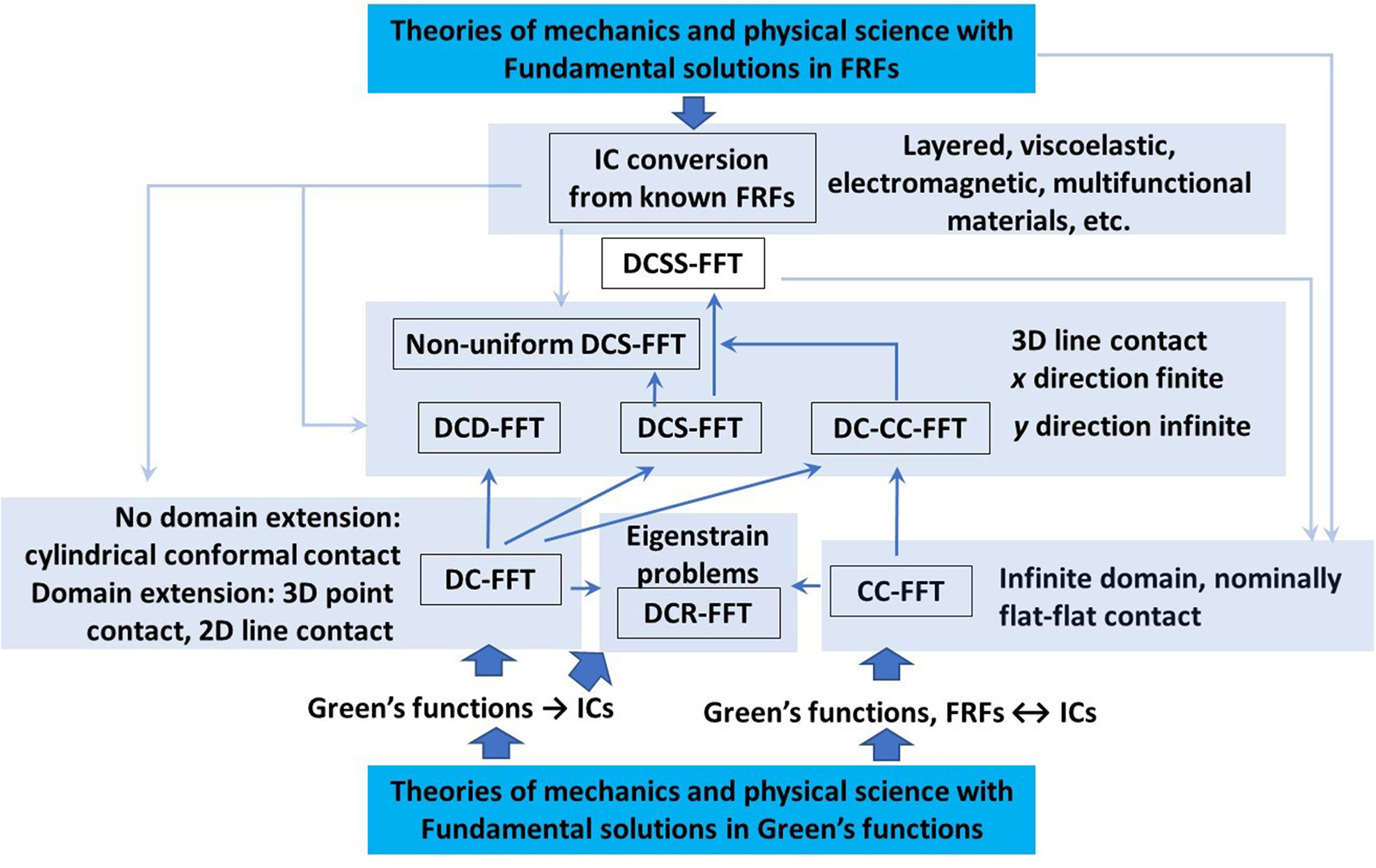
Figure 13. FFT algorithm tree and the application field (light blue) of each. The darker arrow lines indicate the paths of method development while the lighter arrow lines means IC-FRF conversions and information supplies.

Recently, the fast Fourier transform method has been incorporated with the boundary-element method for solving problems with an arbitrary columnar geometry, not confined by the half-space assumption (Benad, 2018, 2019). This further extends the breadth of FFT applications. For the plane-strain problems associated with a columnar geometry formed by extruding a 2D shape in the length direction, e.g., the one solved by Benad (2018, 2019), the FFT solutions have a lower computational complexity, O(n³ log n^1.5), than the inversion of a standard BEM matrix, O(n⁴), where n x n is the total number of surface nodes. These problems are, mathematically, in the same nature as that in Figure 2F, automatically meeting the DC-FFT requirement with no need of the domain extension, as indicated in the first row of Table 1 and Figure 13. Likewise, the FFT method should also be directly applicable to plane-stress problems of a disk-like geometry of any shape.

Limitations and Future Developments

The FFT-based methods mentioned here well fit the solutions of many engineering problems, not limited to mechanical contacts, as long as their model formulations contain convolution and/or correlation, or are solvable in the frequency domain, subjected to the assumptions of small deformation (linear or piecewise linear). So far, for counterformal contacts, the characteristic body dimension, such as radius, should be much larger than that of the contact area; for conformal contacts, bodies involved should have axisymmetry or columnar geometries. Generally, these FFT-based solution approaches are confined by uniform meshes. Although section FFT With Non-uniform Mesh has briefly discussed the use of non-uniform meshes, more work is needed to make the non-uniform-mesh FFT algorithms more flexible and more efficient for contact analyses. Large deformation and the effect of body forces are also among the challenges to further developments of FFT-based methods for contact mechanics.

Data Availability Statement

The original contributions presented in the study are included in the article, open-source codes are available on-line in http://othello.mech.northwestern.edu/qwang/OpenSourceCodeDCFFT/DC-FFTWeb.htm; http://othello.mech.northwestern.edu/qwang/OpenSourceCodeEigenstrainFiledHalf Space/2012Web.htm. Further inquiries can be directed to the corresponding authors.

Author Contributions

QW leads the overall writing, LS is on some of the methods and results in Introduction, FFT Algorithms for 3D Line-Contact Problems, DCR-FFT Algorithm, FFT With Non-uniform Mesh, XZ on IC Conversion From FRFs, SL on technical and algorithm review, and DZ on a part of Frequency Response Functions and ICs and rough surface contact results. All authors contributed to the article and approved the submitted version.

Conflict of Interest

DZ is associated with Tri-Tech Solutions.

The remaining authors declare that the research was conducted in the absence of any commercial or financial relationships that could be construed as a potential conflict of interest.

Acknowledgments

The authors would like to express sincere gratitude to co-workers at the Center for Surface Engineering and Tribology, Northwestern University, Evanston, IL, USA, for years of research on theoretical derivations of fundamental solutions, ICs, and FRFs, and developments and implementations of the FFT-based methods, especially to Drs. W. W. Chen, X. Q. Jin, W.-S. Kim, D. L. Li, Y. C. Liu, Z. Liu, A. Martini, N. Ren, M. J. Rodgers, X. J. Shi, Z. J. Wang, C. J. Yu, M. Q. Zhang, K. Zhou, and Q. H. Zhou, as well as Mr. H. Yu, Chongqing University, China, for their valuable contributions. The authors would also like to thank Professor L. M. Keer, Northwestern University, for long-term collaboration and research discussion, and the journal editor and reviewers for their valuable suggestions on manuscript revision.

References

Ai, X., and Sawamiphakdi, C. (1999). Solving elastic contact between rough surfaces as an unconstrained strain energy minimization by using CGM and FFT techniques. ASME J. Tribol. 121, 639–647. doi: 10.1115/1.2834117

CrossRef Full Text | Google Scholar

Benad, J. (2018). Efficient calculation of the BEM integrals on arbitrary shapes with the FFT. Facta Univ. Ser. Mech. Eng. 16, 405–417. doi: 10.22190/FUME180912034B

CrossRef Full Text | Google Scholar

Benad, J. (2019). Numerical methods for the simulation of deformations and stresses in turbine blade fir-tree connections. Facta Univ. Ser. Mech. Eng. 17, 1–15. doi: 10.22190/FUME190103008B

CrossRef Full Text | Google Scholar

Boucly, V., Nelias, D., Liu, S. B., Wang, Q., and Keer, L. M. (2005). Contact analyses for bodies with frictional heating and plastic behavior. ASME J. Tribol. 127, 355–364. doi: 10.1115/1.1843851

CrossRef Full Text | Google Scholar

Bracewell, R. N. (1978). The Fourier Transform and Its Applications. New York, NY: McGraw Hill.

Google Scholar

Brigham, E. O. (1988). The Fast Fourier Transform and Its Applications. Prentice Hall, NJ: Englewood Cliff.

Chen, W. W., Liu, S. B., and Wang, Q. J. (2008). Fast fourier transform based numerical methods for elasto-plastic contacts of nominally flat surfaces. ASME J. Appl. Mech. 75:011022. doi: 10.1115/1.2755158

CrossRef Full Text | Google Scholar

Chen, W. W., Wang, Q., Zhang, H., and Luo, X. (2011). Semi-analytical viscoelastic contact modeling of polymer-based materials. J. Tribol. 133:041404. doi: 10.1115/1.4004928

CrossRef Full Text | Google Scholar

Choi, H., and Paulino, G. (2008). Thermoelastic contact mechanics for a flat punch sliding over a graded coating/substrate system with frictional heat generation. J. Mech. Phys. Solids 56, 1673–1692. doi: 10.1016/j.jmps.2007.07.011

CrossRef Full Text | Google Scholar

Conry, T. F., and Seireg, A. (1971). A mathematical programming method for design of elastic bodies in contact. ASME J. Appl. Mech. 38, 387–392. doi: 10.1115/1.3408787

CrossRef Full Text | Google Scholar

Eshelby, J. D. (1957). The determination of the elastic field of an ellipsoidal inclusion, and related problems. Proc. R. Soc. A 241, 376–396. doi: 10.1098/rspa.1957.0133

CrossRef Full Text | Google Scholar

Goryacheva, I. G., and Sadeghi, F. (1995). Contact characteristics of a rolling/sliding cylinder and a viscoelastic layer bonded to an elastic substrate. Wear 184, 125–132. doi: 10.1016/0043-1648(94)06561-6

CrossRef Full Text | Google Scholar

Hu, Y. Z., Barber, G. C., and Zhu, D. (1999). Numerical analysis for the elastic contact of real rough surfaces. Tribol. Trans. 42, 443–452. doi: 10.1080/10402009908982240

CrossRef Full Text | Google Scholar

Jin, X., Keer, L. M., Wang, Q., and Chez, E. (2013). “Conjugate gradient method for contact analysis,” in Encyclopedia of Tribology, eds Q. Wang and Y. W. Chung (New York, NY; Heidelberg Dordrecht, London: Springer), 467.

Google Scholar

Johnson, K. L. (1987). Contact Mechanics. London: Cambridge University Press.

Google Scholar

Ju, Y. Q., and Farris, T. N. (1996). Spectral analysis of two-dimensional contact problems. ASME J. Tribol. 118, 320–328. doi: 10.1115/1.2831303

CrossRef Full Text | Google Scholar

Kalker, J. J. (1986). Numerical calculation of the elastic field in a half-space. Commun. Appl. Num. Methods 2, 401–410. doi: 10.1002/cnm.1630020412

CrossRef Full Text | Google Scholar

Kalker, J. J., and van Randen, Y. (1972). A minimum principle for frictionless elastic contact with application to non-hertzian half space contact problems. J. Eng. Math. 6, 193–206. doi: 10.1007/BF01535102

CrossRef Full Text | Google Scholar

Ke, L., and Wang, Y. (2006). Two-dimensional contact mechanics of functionally graded materials with arbitrary spatial variations of material properties. Int. J. Solids Struct. 43, 5779–5798. doi: 10.1016/j.ijsolstr.2005.06.081

CrossRef Full Text | Google Scholar

Liu, S. (2013). Numerical simulation of conformal contacts involving both interference and clearance. Tribol. Transac. 56, 867–878. doi: 10.1080/10402004.2013.806686

CrossRef Full Text | Google Scholar

Liu, S., and Chen, W. (2012). Two-dimensional numerical analyses of double conforming contacts with effect of curvature. Int. J. Solids Struct. 49, 1365–1374. doi: 10.1016/j.ijsolstr.2012.02.019

CrossRef Full Text | Google Scholar

Liu, S., Chen, W. W., Hua, D., and Wang, Q. (2007). Tribological modeling: application of fast fourier transform. Tribol. Int. 40, 1284–1293. doi: 10.1016/j.triboint.2007.02.004

CrossRef Full Text | Google Scholar

Liu, S., and Hua, D. Y. (2009). Three-dimensional semiperiodic line contact–periodic in contact length direction. J. Tribol. 131:021408. doi: 10.1115/1.3084237

CrossRef Full Text | Google Scholar

Liu, S., and Wang, Q. (2002). Studying contact stress fields caused by surface tractions with a discrete convolution and fast fourier transform algorithm. ASME J. Tribol. 124, 36–45. doi: 10.1115/1.1401017

CrossRef Full Text | Google Scholar

Liu, S., Wang, Q., and Liu, G. (2000). A versatile method of discrete convolution and FFT (DC-FFT) for contact analyses. Wear 243, 101–111. doi: 10.1016/S0043-1648(00)00427-0

CrossRef Full Text | Google Scholar

Liu, S. B. (2001). Thermomechanical contacts of rough surfaces [Ph. D. thesis]. Northwestern University, Evanston, IL, United States.

Liu, S. B., Jin, X. Q., Wang, Z. J., Keer, L. M., and Wang, Q. (2012). Analytical solution for elastic fields caused by eigenstrains in a half-space and numerical implementation based on FFT. Int. J. Plasticity 35, 135–154. doi: 10.1016/j.ijplas.2012.03.002

CrossRef Full Text | Google Scholar

Liu, S. B., and Wang, Q. (2005). Elastic fields due to eigenstrains in a half-space. ASME J. Appl. Mech. 72, 871–878. doi: 10.1115/1.2047598

CrossRef Full Text | Google Scholar

Liu, S. B., Wang, Q., Rodgers, M. J., Keer, L. M., and Cheng, H. S. (2002). Temperature distributions and thermoelastic displacements in moving bodies. Comput. Model. Eng. Sci. 3, 465–481. doi: 10.3970/cmes.2002.003.465

CrossRef Full Text | Google Scholar

Liu, Y., Chen, W., Liu, S., Zhu, D., and Wang, Q. (2007). An elastohydrodynamic lubrication model for coated surfaces in point contacts. J. Tribol. 129, 509–516. doi: 10.1115/1.2736433

CrossRef Full Text | Google Scholar

Liu, Y., Wang, Q., Hu, Y., Wang, W., and Zhu, D. (2006). Effects of differential schemes and mesh density on EHL film thickness in point contacts. ASME J. Tribol. 128, 641–653. doi: 10.1115/1.2194916

CrossRef Full Text | Google Scholar

Liu, Y., Wang, Q., Zhu, D., Wang, W., and Hu, Y. (2009). Effects of differential scheme and viscosity model on rough-surface point-contact isothermal EHL. J. Tribol. 131:044501. doi: 10.1115/1.2842245

CrossRef Full Text | Google Scholar

Liu, Z., Gu, T., Pickens, D., Nishino, T., and Wang, Q. (2020). Model assisted housing profile design for improved apex seal lubrication using a finite-length roller EHL model. Rev. J. Tribol.

Londhe, N. D., Arakere, N. K., and Subhash, G. (2018). Extended hertz theory of contact mechanics for case-hardened steels with implications for bearing fatigue life. ASME J. Tribol. 140:021401. doi: 10.1115/1.4037359

CrossRef Full Text | Google Scholar

Love, A. E. H. (1929). Stress produced in a semi-infinite solid by pressure on part of the boundary. Philod. Trans. R. Soc. A228, 337–420. doi: 10.1098/rsta.1929.0009

CrossRef Full Text | Google Scholar

Morrison, N. (1994). Introduction to Fourier Analysis. New York, NY: John Wiley and Sons.

Google Scholar

Mura, T. (1993). Micromechanics of Defects in Solids, 2nd Edn. Dordrecht: Kluwer Academic Publishers.

Google Scholar

Nogi, T., and Kato, T. (1997). Influence of a hard surface layer on the limit of elastic contact-part i: analysis using a real surface model. ASME J. Tribol. 119, 493–500. doi: 10.1115/1.2833525

CrossRef Full Text | Google Scholar

Oppenheim, A., Schafer, R., and Buck, J. (1999). Discrete-Time Signal Processing, 2nd Edn, Pearson, Upper Saddle River, NJ.

Google Scholar

Pohrt, R., and Popov, V. L. (2015). Adhesive contact simulation of elastic solids using local mesh-dependent detachment criterion in boundary elements method. Facta Univ. Ser. Mech. Eng. 13, 3–10.

Google Scholar

Polonsky, I. A., and Keer, L. M. (1999). A numerical method for solving rough contact problems based on the multi-level multi-summation and conjugate gradient techniques. Wear 231, 206–219. doi: 10.1016/S0043-1648(99)00113-1

CrossRef Full Text | Google Scholar

Polonsky, I. A., and Keer, L. M. (2000). Fast methods for solving rough contact problems: a comparative study. ASME J Tribol. 122, 36–41. doi: 10.1115/1.555326

CrossRef Full Text | Google Scholar

Popov, V. L., Pohrt, R., and Li, Q. (2017). Strength of adhesive contacts: influence of contact geometry and material gradients. Friction 5, 308–325. doi: 10.1007/s40544-017-0177-3

CrossRef Full Text | Google Scholar

Press, W. H., Teukolsky, S. A., Vetterling, W. T., and Flannery, B. P. (1992). Numerical Recipes in Fortran 77-The Art of Scientific Computing, 2nd Edn. Cambridge: Cambridge University Press.

Google Scholar

Putignano, C., Carbone, G., and Dini, D. (2015). Mechanics of rough contacts in elastic and viscoelastic thin layers. Int. J. Solids Struct. 69, 507–517. doi: 10.1016/j.ijsolstr.2015.04.034

CrossRef Full Text | Google Scholar

Ren, N., Zhu, D., Chen, W. W., Liu, Y., and Wang, Q. (2009). A three-dimensional deterministic model for rough surface line-contact EHL. J. Tribol. 131:011501. doi: 10.1115/1.2991291

CrossRef Full Text | Google Scholar

Ren, N., Zhu, D., Chen, W. W., and Wang, Q. (2010). Plasto-Elastohydrodynamic Lubrication (PEHL) in point contact. J. Tribol. 132:031501. doi: 10.1115/1.4001813

CrossRef Full Text | Google Scholar

Rey, V., Anciaux, G., and Molinari, J.-F. (2017). Normal adhesive contact on rough surfaces: efficient algorithm for FFT-based BEM resolution. Comput Mech. 60, 69–81. doi: 10.1007/s00466-017-1392-5

CrossRef Full Text | Google Scholar

Stanley, H. M., and Kato, T. (1997). An FFT-based method for roughness surface contact. ASME J. Tribol. 119, 481–485. doi: 10.1115/1.2833523

CrossRef Full Text | Google Scholar

Stepanov, F., and Torskaya, E. (2018). Modeling of sliding of a smooth indenter over a viscoelastic layer coupled with a rigid base. Mech. Solids 53, 60–67. doi: 10.3103/S0025654418010077

CrossRef Full Text | Google Scholar

Sun, L. (2020). Advanced FFT Algorithms for Contact of Materials with Inhomogeneities and Their Applications. [Ph.D. thesis]. Northwestern Polytechnical University, Xian, China.

Sun, L., Wang, Q., Zhang, M., Zhao, N., Keer, L. M., Liu, S. B., et al. (2020). Discrete convolution and FFT method with summation of influence coefficients (DCS-FFT) for three-dimensional contact of inhomogeneous materials. Comput. Mech. 65, 1509–1529. doi: 10.1007/s00466-020-01832-2

CrossRef Full Text | Google Scholar

Walker, J. S. (1996). Fast Fourier Transforms, 2nd Edn. Boca Raton, FL: CRC Press.

PubMed Abstract | Google Scholar

Wang, F. C., and Jin, Z. M. (2004). Prediction of elastic deformation of acetabular cups and femoral heads for lubrication analysis of artificial hip joints. Proc. Inst. Mech. Eng. Pt. J. J. Eng. Tribol. 218, 201–209. doi: 10.1243/1350650041323331

CrossRef Full Text | Google Scholar

Wang, Q., and Zhu, D. (2019). Interfacial Mechanics, Theories and Methods for Contact and Lubrication. Boca Raton, FL; London, New York, NY: CRC Press.

PubMed Abstract | Google Scholar

Wang, W.-Z., Wang, H., Liu, Y.-C., Hu, Y.-Z., and Zhu, D. (2003). A comparative study of the methods for calculation of surface elastic deformation. Proc. Inst. Mech. Eng. Pt. J. J. Eng. Tribol. 217, 145–152. doi: 10.1243/13506500360603570

PubMed Abstract | CrossRef Full Text | Google Scholar

Wang, Y., Zhang, X., Shen, H., Liu, J., and Zhang, B. (2020). Couple stress-based 3D contact of elastic films. Int. J. Soilds Struct. 191–192, 449–463. doi: 10.1016/j.ijsolstr.2020.01.005

CrossRef Full Text | Google Scholar

Wang, Z., Jin, X., Keer, L. M., and Wang, Q. (2013b). Novel model for partial-slip contact involving a material with inhomogeneity. J. Tribol. 135:041401. doi: 10.1115/1.4024548

CrossRef Full Text | Google Scholar

Wang, Z., Yu, H., and Wang, Q. (2017a). Layer-substrate system with imperfect bonding interface: coupled dislocation-like and force-like conditions. Int. J. Solids Struct. 122–123, 91–109. doi: 10.1016/j.ijsolstr.2017.06.004

CrossRef Full Text | Google Scholar

Wang, Z., Yu, H., and Wang, Q. (2017b). Layer-substrate system with an imperfectly bonded interface: spring-like condition. Int. J. Mech. Sci. 134, 315–335. doi: 10.1016/j.ijmecsci.2017.10.028

CrossRef Full Text | Google Scholar

Wang, Z. J., Jin, X. Q., Zhou, Q. H., Ai, X. L., Keer, L. M., and Wang, Q. (2013a). An efficient numerical method with a parallel computational strategy for solving arbitrarily shaped inclusions in elasto-plastic contact problems. ASME J. Tribol. 135:031401. doi: 10.1115/1.4023948

CrossRef Full Text | Google Scholar

Wang, Z. J., Yu, C., and Wang, Q. (2015). Model for elastohydrodynamic lubrication of multilayered materials. J. Tribol. 137:011501. doi: 10.1115/1.4028408

CrossRef Full Text | Google Scholar

Wang, Z. J., and Zhang, Y. (2019). An efficient numerical model of elastohydrodynamic lubrication for transversely isotropic materials. ASME J. Tribol. 141:091501. doi: 10.1115/1.4043902

CrossRef Full Text | Google Scholar

Wang, Z. J., Zhu, D., and Wang, Q. (2014). Elastohydrodynamic lubrication of inhomogeneous materials using the equivalent inclusion method. J. Tribol. 136:021501. doi: 10.1115/1.4025939

CrossRef Full Text | Google Scholar

Yu, C. J., Wang, Z. J., Liu, G., Keer, L. M., and Wang, Q. (2016). Maximum von mises stress and its location in trilayer materials in contact. ASME J. Tribol. 138:041402. doi: 10.1115/1.4032888

CrossRef Full Text | Google Scholar

Yu, C. J., Wang, Z. J., and Wang, Q. (2014). Analytical frequency response functions for contact of multilayered materials. Mech. Mater. 76, 102–120. doi: 10.1016/j.mechmat.2014.06.006

CrossRef Full Text | Google Scholar

Zhang, H. B., Wang, W. Z., Zhang, S. G., and Zhao, Z. Q. (2017). Elastohydrodynamic lubrication analysis of finite line contact problem with consideration of two free end surfaces. J. Tribol. 139:031501. doi: 10.1115/1.4034248

CrossRef Full Text | Google Scholar

Zhang, H. B., Wang, W. Z., Zhang, S. G., and Zhao, Z. Q. (2018). Semi-analytic solution of three-dimensional temperature distribution multilayered materials based on explicit frequency response functions. Int. J. Heat Mass Transfer 118, 208–222. doi: 10.1016/j.ijheatmasstransfer.2017.10.118

CrossRef Full Text | Google Scholar

Zhang, M. Q., Zhao, N., Wang, Z. J., and Wang, Q. (2018). Efficient numerical method with a dual-grid scheme for contact of inhomogeneous materials and its applications. Comput. Mech. 62, 991–1007. doi: 10.1007/s00466-018-1543-3

CrossRef Full Text | Google Scholar

Zhang, X., and Wang, Q. (2019). A SAM-FFT based model for 3d steady-state elastodynamic frictional contacts. Int. J. Solids Struct. 170, 53–67. doi: 10.1016/j.ijsolstr.2019.04.028

CrossRef Full Text | Google Scholar

Zhang, X., and Wang, Q. (2020). “Thermoelastic Contacts of Layered Materials with Interface Imperfections,” Int. J. Mech. Sci. 186:105904. doi: 10.1016/j.ijmecsci.2020.105904

CrossRef Full Text | Google Scholar

Zhang, X., Wang, Q., Harrison, K., Roberts, S., and Harris, S. J. (2019). Rethinking how external pressure can suppress dendrites in lithium metal batteries. J. Electrochem. Soc. 166, A3639–A3652. doi: 10.1149/2.0701914jes

CrossRef Full Text | Google Scholar

Zhang, X., Wang, Q., Harrison, K. L., Roberts, S. A., and Harris, S. J. (2020c). Pressure-driven interface evolution in solid state lithium metal batteries. Cell Rep. Phys. Sci. (2020) 1:100012. doi: 10.1016/j.xcrp.2019.100012

CrossRef Full Text | Google Scholar

Zhang, X., Wang, Q., and He, T. (2020a). Triansient and steady-state viscoelastic contact response of layer-substrate systems with interfacial imperfections. J. Mech. Phys. Solids (2020).

Google Scholar

Zhang, X., Wang, Q., He, T., Liu, Y., Li, Z., Jim, H. J., et al. (2020b). Fully coupled modeling of thermo-viscoelastic contacts of layered materials. Mech. Mater.

Google Scholar

Zhang, X., Wang, Z. J., Shen, H. M., and Wang, Q. (2017). Frictional contact involving a multiferroic thin film subjected to surface magnetoelectroelastic effects. Int. J. Mech. Sci. 131–132, 633–648. doi: 10.1016/j.ijmecsci.2017.07.039

CrossRef Full Text | Google Scholar

Zhang, X., Wang, Z. J., Shen, H. M., and Wang, Q. (2018). An efficient model for the frictional contact between two multiferroic bodies. Int. J. Solids Struct. 130–131, 133–152. doi: 10.1016/j.ijsolstr.2017.10.004

CrossRef Full Text | Google Scholar

Zhou, Q. H., Jin, X. Q., Wang, Z. J., Yang, Y., Wang, J. X., Keer, L. M., et al. (2016). A mesh differential refinement scheme for solving elastic fields of half-space inclusion problems. Tribol. Int. 93A, 124–136. doi: 10.1016/j.triboint.2015.09.009

CrossRef Full Text | Google Scholar

Zhou, Y., and Lee, K. (2013). Theory of sliding contact for multiferroic materials indented by a rigid punch. Int. J. Mech. Sci. 66, 156–67. doi: 10.1016/j.ijmecsci.2012.11.004

CrossRef Full Text | Google Scholar

Zhu, D., Martini, A., Wang, W., Hu, Y., Lisowsky, B., and Wang, Q. (2007). Simulation of sliding wear in mixed lubrication. J. Tribol. 129, 544–552. doi: 10.1115/1.2736439

CrossRef Full Text | Google Scholar

Appendix

Contact Conditions

The contact of two bodies, (1) and (2), should satisfy the complementary “gap-G” and “flux-F” conditions, shown below, with 1, 2, 3 for x, y, z.

$\begin{array}{l}{G}_3(x_1,x_2)>0;F_{33}^{*}=0if(x_1,x_2)\notin A_c\\ G_3(x_1,x_2)=0;F_{33}^{*}>0if(x_1,x_2)\in A_c& (\mathrm{A1})\end{array}$

where $F_{33}^{*}=-p$ is the contact pressure, and $G_3={\overline{B}}^{(1)}(x_1,x_2)+u_3^{(1)}(x_1,x_2)+{\overline{B}}^{(2)}(x_1,x_2)+u_3^{(2)}(x_1,x_2)-\overline{g}$ with $g(x_1,x_2)=\left({\overline{B}}^{(1)}(x_1,x_2)+u_3^{(1)}(x_1,x_2)\right)+\left({\overline{B}}^{(2)}(x_1,x_2)+u_3^{(2)}(x_1,x_2)\right),$ $\overline{g}=\frac{1}{N_c}\left[{\displaystyle \sum _{(i,j)\in A_c}g(x_1,x_2)}\right],$ where u₃ is u_z given in Equation (3) or (10), ${\overline{B}}^{(i)}$is for the geometry of body i, and N_c is the total nodes in the contact area A_c.

The contact area adjustment can be made through the following.

$\begin{array}{l}\text{If }{G}_3(x_1,x_2)<0,\text{ make }{G}_3(x_1,x_2)=0\text{ and}\\ \begin{array}{l}\text{ add point }(x_1,x_2)\text{ to }{A}_c\end{array}& (\mathrm{A2})\end{array}$

The overall the load balance is

$\begin{array}{ll}{\displaystyle {\int }_{A_c}}{F}_{33}^{*}\text{d}A={\overline{P}}_M& (\mathrm{A3})\end{array}$

where ${\overline{P}}_M$ is the normal load. The contact area and pressure distributions can be solved by using the conjugate gradient method (CGM) (Polonsky and Keer, 1999).

In addition, the contact should also satisfy the interfacial conditions for fluxes.

$\begin{array}{l}{F}_{3J}^{*}=0\text{ if }(x_1,x_2)\notin A_c\\ F_{3J}^{*(1)}(x_1,x_2)=-F_{3J}^{*(2)}(x_1,x_2)\text{ if }(x_1,x_2)\in A_{c}J=1,2,3& (\mathrm{A4})\end{array}$

where $F_{3J}^{*(i)}(x_1,x_2)=\left\{{\overline{t}}_{M1},{\overline{t}}_{M2},-p\right\},\text{and }{\overline{t}}_{Mi}$ means the surface tangential tractions in the x₁ and x₂ directions. These conditions are also applicable to other multifield contact problems (Wang and Zhu, 2019).