Evaluation of a Double-Entry Turbine Model Coupled With a One-Dimensional Calibrated Engine Model at Engine Full Load Curves

Introduction

With growing interest in global environmental issues, the automotive manufacturers are facing increasing challenges to reduce the gaseous emissions coming from the internal combustion engines (Haq and Weiss, 2016). Moreover, also to meet the strict emission legislation year by year (Wang et al., 2017). Satisfying these more tightening regulations cost-effectively is the most crucial challenge for automotive makers nowadays. Despite the rapid growth of electric car sales in recent years, one should note that the battery electric vehicles (BEV) have massive CO₂ footprints when analysed from cradle-to-grave (Romare and Dahllöf, 2017). Additionally, considering and targeting to more extensive use of electric drive powertrain in future still requires the development of the appropriate grid and charging infrastructure. It also needs the essential improvements in battery energy density for having long-range drives. These elements are crucial for effective market penetration of electric vehicles, including enhancements in cost-effectiveness as well as technology. Roadmaps have been drawn to anticipate the potential automotive technology trends by 2050 (Heywood et al., 2015; Kalghatgi, 2018). It was predicted that a mix of solutions would characterize future mobility. The plug-in hybrid powertrain and small capacity turbocharged engines will play a significant part of the passenger cars need in decades ahead (Kalghatgi, 2018). In order to compete with an electric powertrain, automotive engineers are developing new internal combustion engines to be environment friendly. At the same time, keeping the vehicle performance and also having sufficiently attractive fuel consumption to satisfy the customer’s requirement. In recent years, automotive OEMs are seeing much interest in using the double-entry turbines, especially for four-cylinder turbocharged petrol engines with the wide valves overlap period in their timing diagram or six-cylinder compression ignition engines (Zhu and Zheng, 2017). They have the advantages of utilizing the pulse energy coming from the engine exhaust and minimizing the interferences between the cylinders during the exhaust process (engine pumping losses).

Many research studies have already been carried out on the performance of double-entry turbines coupled with the internal combustion engines. Walkingshaw et al. (2015) compared the twin-entry and dual-volute turbine with a single-entry turbine with a focus of on-engine turbine performance. From the results, it was concluded that both twin-entry and dual-volute turbines offer notable improvements at engine part-load conditions. The unsteady performance parameters of the twin-entry turbine at real engine conditions have been experimentally and numerically studied by many researchers (Rajoo et al., 2012; Serrano et al., 2019a). Zhu and Zheng (2017) compared the engine performance with symmetric and asymmetric twin-entry turbines and concluded that asymmetric turbine has a more significant impact on the fuel economy and engine emissions.

Nowadays, automotive manufacturers are focusing on a wide range of engine operating conditions which are different from a regular full-load performance. To obtaining an optimum matching between the turbocharger and internal combustion engines, automotive manufacturers are relying on one-dimensional engine cycle simulation tools to predict and study the effect of various parameters on engine performance. 1D simulation codes make possible the calculation of gas dynamics engine behaviour at low computational costs. Furthermore, the method also shows an important approach to simulate the unsteady performance of the turbine (Serrano et al., 2008; Ding et al., 2017). Wei et al. (2020) studied the influence of twin-entry turbine configuration on the engine performance with a one-dimensional turbine model with two entries coupled to a 1D engine model. From the study, it was concluded that the swallowing capacity of the twin-entry turbine varies dramatically with engine conditions, which is a similar function of variable geometry turbine. Costall et al. (2010) developed a model for twin-entry turbines and solved using a gas dynamics code. The pulse flow performance of a twin-entry turbine under unequal and full admission conditions are analysed and suggested that for full admission flow states, a twin-entry turbine can be modelled as a simplified single entry model, whereas for unequal flows, a more complex model is necessary.

Typically, the steady flow maps of double-entry turbines are only available under full admission conditions (where the flow is the same in both entries of the turbine), and they are not enough for the engine simulation purposes. In fact, the exhaust pulses feeding each entry of the turbine will be timed, so that they are out of phase with other; as a result, double-entry turbines spend little time in full admission and majority of the time with unequal flows in their entries. Therefore, the turbine maps should also cover the necessary flow conditions such as unequal and partial admissions between their entries. Mainly, turbine models are based on steady flow maps, with information about the mass rate and isentropic efficiency. They solve the system of equations by assuming a quasisteady behaviour. In engine part loads and transient conditions, the turbocharger turbine works at off-design conditions (Dale and Watson, 1986). Therefore, this behaviour cannot be able to catch by a standard turbine map provided by the manufacturers. Therefore, turbine models should be capable of simulating the real-life engine conditions, so that the prediction of exhaust gas mass flow and the pressure drop across the turbine and energy transfer to the compressor are essential. In this regards, turbine map extrapolation tools are necessary when using one-dimensional modelling tools to predict the system behaviour outside of the turbine design operative conditions (Martin et al., 2009). In the literature, there are good examples about how to model the single entry radial inflow turbines in turbocharged engines and with the one-dimensional gas dynamic codes. But the corresponding twin-entry and dual-volute turbine modelling procedures are not predictive enough for calculating the entire gas exchange process of internal combustion engines considering unsteady flow, the whole engine map (load and speed), and engine load and speed transients. It is mainly due to the unequal flow admission conditions, which generate an additional degree of freedom concerning the well-known single entry vaned or vaneless turbines.

In this paper, the CMT double-entry turbocharger model (CMT-DETCM), which is developed in the previous work (Serrano et al., 2020b), has been evaluated using the whole one-dimensional calibrated engine model at full load curves. Systematizing the performance of maps of twin/dual-volute turbines gave the ability to model any double-entry turbine as if it is formed of two VGTs and, furthermore, made it possible to extrapolate the turbine-reduced mass flow and efficiency maps to off-design conditions. The model is predictive either in partial or unequal admission conditions using as inputs: the mass flow ratio and total temperature ratio between the branches; the expansion ratio and blade speed ration in each branch. These six inputs are generally instantaneously provided by one-dimensional gas-dynamic codes. Therefore, the novelty of the model is its ability to be used in a quasisteady way for any double-entry turbines performance prediction. This can be achieved instantaneously as turbines are calculated under pulsating and uneven flow conditions at turbocharged engines. The theoretical development of the double-entry turbine model used in this work has been briefly explained in Annex.

The explained model was integrated into an in-house one-dimensional gas dynamic simulation tool called VEMOD (Martin et al., 2018). The complete adaptation of the double-entry turbine model to be used in a quasisteady way was detailed in (Serrano et al., 2019b). The double-entry turbine model considers pressure pulses and reflections during the full engine simulation. They are solved by Euler’s classical governing equations using a finite-volume approach and computed using a Godunov scheme (Serrano et al., 2019b; Soler Blanco, 2020). Figure 1 shows the double-entry turbine model computational domain. The flow in stations C, D, and E is determined using a technique described in (Serrano et al., 2008), to split the expansion ratio in the turbine between the stator and rotor nozzles (stations C and E, respectively). Furthermore, heat transfer effects are taken into consideration as an energy source term, by changing the temperature of flow when it is passing between stations C and E. An extra energy sink term is introduced in the volume D equal to the power output of the turbine at each time step. The extrapolated turbine maps by the models described in (Serrano et al., 2020b) were used to compute the stator (C) and rotor (E) nozzles using the techniques described in (Serrano et al., 2008), and the efficiency is quasisteadily obtained as represented in (Serrano et al., 2020b). Gas dynamic effects on the compressor side are modelled using two volumes and the connecting tube as described in (Galindo et al., 2019). Moreover, few different submodels for estimating the mechanical losses (Serrano et al., 2013) and heat transfer effects (Payri et al., 2014; Serrano et al., 2015b) in the turbochargers are also taken into account during the simulation. All the model information were transferred into GT-Power software by creating an external library link. By using this library link, the CMT-DETCM model can be able to simulate in the GT-Power software as a gas stand or just coupling to the engine model.

FIGURE 1

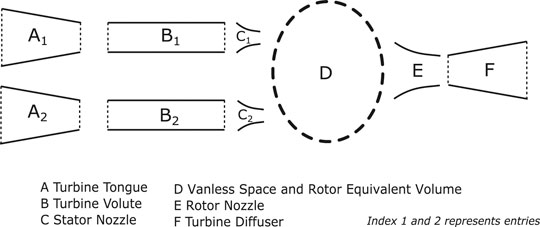
FIGURE 1. Double entry turbine model computational domain.

The CMT-DETCM model was validated beforehand with the data obtained from the gas stand. The data was acquired with more accurate instrumentation, placing several thermocouples at the inlet and outlet of the turbine for temperature measurement. More details about this work can be found in (Samala, 2020). It is worth highlighting that the internal and external heat transfer models used in this work are previously developed and calibrated for a single/VGT turbocharger. However, the heat exchange process in double-entry turbines will be different due to the imbalance of flows and different levels of temperatures coming from the engine cylinders to the turbine inlets. Furthermore, one of the entries will be closed to shaft housing and another exposed mainly to the ambient; accordingly, the heat transfer from each entry will be different to the other turbocharger elements. However, in this work, the heat transfer effects in double-entry turbines were not the primary objective. Therefore, the first approximation of heat transfer in double-entry turbochargers was calculated in a similar way to the single entry turbocharger thermal model based on the electric analogy as described in (Samala, 2020).

This paper is divided into three parts. First, the experimental works carried out with a dual-volute mixed flow turbine (T$\#$1DVM) with a gasoline engine in a test rig will be discussed. Then, the one-dimensional engine model calibration procedure will be explained. Finally, engine simulations with the proposed CMT-DETCM turbocharger model have been performed to see the model prediction with engine conditions.

Engine Experimental Campaign

The test bench used to validate the CMT-DETCM model is a standard test rig which is designed by CMT-Motores Térmicos to study the internal combustion engines up to 200kW of power. The facility allows to control and rate the engine performance in steady and transient conditions. Figure 2 shows the scheme of the engine test facility and the sensor instrumentation.

FIGURE 2

FIGURE 2. The layout of the engine test cell and the sensor instrumentation.

The engine is coupled with the asynchronous dynamometer (APA). It is fixed to the test-bed using metallic beams joined by screw or welding. The construction of the bed is designed in a way that it prevents longitudinal movement of the engine and makes easier the alignment with the dynamometer. The engine speed and load rate are controlled by the automatic acceleration system called throttle and the dynamometer. They are introduced into the control and data acquisition system called PUMA. The dynamometer offers essential resistance torque for the engine to test at different loads. The heat generated by the engine was controlled through water cooling systems. The heat exchange systems control the thermal state of the different fluids such as water cooling, air intake, fuel, and oil. The mass flow rate of the coolant is adjusted by an electric valve commanded by a PID controller.

A turbocharged spark-ignition internal combustion engine with a dual-volute mixed flow turbine (T$\#$1DVM) was mounted on the facility. It is a four-cylinder engine with a displacement of 1.3 L and has a variable valve timing (VVT), direct injection system, and Euro 6 calibration. Some of the main technical characteristics of this engine are presented in Table 1. The test facility is controlled automatically by a control system called PUMA V5. It allows acquisition of a set of variables that characterize the behaviour of the different systems of the engine. The data obtained by the sensors through this system are within a frequency of 10–20 Hz. In order to record the instantaneous measurements at the intake manifold and in the cylinders, Kistler type 4045A and AVL ZI33 sensors were used. The AVL sensor ZI33 is a spark plug with an integrated pressure sensor. In an engine test bench, the instantaneous pressure installation at the exhaust manifold is more restrictive due to the design and alignment position of the dual-volute turbine with the engine. Furthermore, there were no pressure probes on the turbine as well. Therefore, a low-speed piezoresistive pressure sensor of Kistler type 4262A was installed. For temperature measurements, either K-type thermocouples or thermoresistances Pt100 are used.

TABLE 1

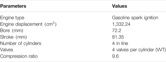
TABLE 1. Engine main specifications.

It is worth highlighting that, on the exhaust manifold, two pressure and two temperature sensors were installed instead of one as shown in Figure 3, due to both branches. Two of the sensors record pressure and temperature coming from cylinders 2 and 3, which are connected to the long volute branch, as shown in Figure 4. The other two sensors are for cylinders 1 and 4, which areconnected to the short volute branch, as shown in Figure 4. This way, it is possible to measure the variables in both branches and helps in the validation of the model. The fuel flow rate is measured using an AVL fuel balance system (AVL733S). The torque of the engine is measured through load cell coupled to the dynamometer. The crankshaft rotation angle and engine speed are measured by an optical angular encoder and Kistler 2613B sensor. Finally, the electronic control unit (ECU) calculates some variables depending on the engine working conditions. These variables are measured by specific control software called INCA V5.

FIGURE 3

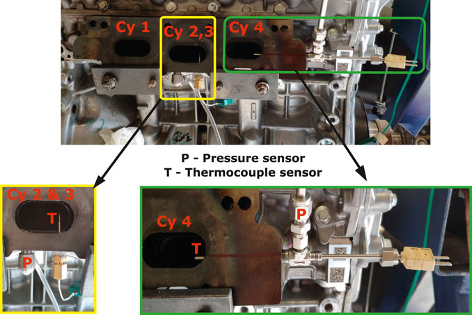
FIGURE 3. Pressure and temperature sensor instrumentation on the exhaust line of the engine.

FIGURE 4

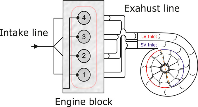
FIGURE 4. Dual volute turbine connection with the engine cylinders.

Test Methodology and Results

Turbocharger T$\#$1DVM is a wastegate turbine and has a special valve called scroll connection valve (SCV) for communicating the flows between branches. Both wastegate and SCV are controlled with a cylindrical type of valve which is connected to a stepper motor. When the cylindrical valve rotates, it has four different functions:

• Wastegate can be opened totally without opening the SCV

• Both wastegate and SCV are closed

• SCV can be opened with wastegate closed

• Both SCV and wastegate are opened

The function of the cylindrical valve is shown in Figure 5. The position of this valve was controlled externally using a PXI^TM system from National Instruments. Nine steady-state engine full load points at different speeds have been measured with the T$\#$1DVM turbocharger. Each full load point were tested twice by keeping SCV totally closed (function in Figure 5A) and with SCV totally open (function in Figure 5C). The target was to reach the maximum engine performance for each full load point in both the tests. While testing, the spark advance was optimized to keep the knock under control. This is carried out by using the knock detection and combustion diagnosis software which is designed by CMT-Motores Térmicos based on the in-cylinder pressure analysis, as it is described by Pla et al. (2020). The ECU controls air-to-fuel ratio (AFR) based on the estimation of turbine inlet temperature to protect the overheating of the turbine. Engine and turbocharger working limits provided by the manufacturers were kept under control.

FIGURE 5

FIGURE 5. Wastegate and SCV flow areas with the cylindrical valve opening.

Figure 6 shows the test results of the engine at full loads for both configurations (i.e., SCV closed and open) and are plotted against the engine speeds. From Figure 6, the following conclusions can be obtained:

• Comparing the torque of engine in both configurations (i.e., SCV closed and open), different situations can be seen depending on the engine speed. Initially (at 1,250 rpm), some benefits can be achieved by operating in the SCV closed condition. At 1,500 rpm, the performance in both configurations is equivalent. From that point on, SCV closed configuration is always detrimental with respect to the open one, especially once the engine speed exceeds 3,000 rpm.

• The benefit observed for SCV closed at 1,250 rpm comes from a higher boost pressure capability in this condition (around 0.4 bar). In the SCV open case, the wastegate valve is fully closed, and the turbine operating limits the boost pressure provided by the compressor. Instead, in the closed SCV, the separation of the exhaust pulses arriving to the turbine from each cylinder makes it possible to deliver more power to the compressor, reaching a final boost pressure which is limited by the compressor map itself, so the wastegate valve is slightly open to avoid surge occurrence.

• At intermediate speeds (1,500–4,000 rpm), the SCV open configuration is affected by the compressor outlet temperature limitation, set at 170°C. This means that the maximum acceptable pressure ratio in the compressor was achieved. Instead, the boost pressure for SCV closed configuration did not reach the same boost pressure level after 2000 rpm since the turbine inlet pressure increased more steeply and led to lower torque potential.

• In the SCV closed configuration test, the turbine inlet pressure in both volutes is unequal. This means that the wastegate flow area of each branch (Figure 5) is different when the SCV is closed. But, when the SCV is open, the pressure levels in both volutes are similar due to the wastegate flow area is same for both branches (Figure 5). Furthermore, there is a communication of flows between the branches. It is worth highlighting that the turbine inlet pressure of LV and SV measured in both test configuration is the average of two pulses. Moreover, the turbine inlet temperature measured in each branch comes from the energy of 2 cylinders instead of 4.

• The measured temperature in short volute is much lower than long volute. In general, the temperature difference between the branches could not be much higher, as seen in the experiments. The problem of measuring the low temperature in the short volute can be due to the position of a thermocouple sensor in cylinder 4 (Figure 3).

FIGURE 6

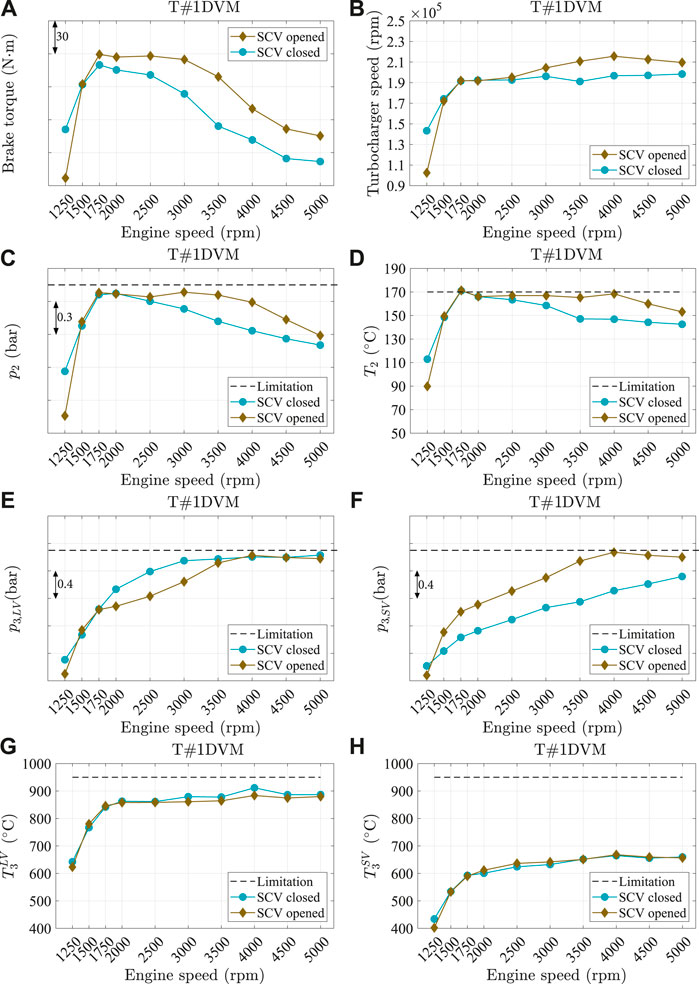
FIGURE 6. Dual volute mixed flow turbine engine test results at full load steady conditions. (A) Engine brake torque; (B) turbocharger speed; (C) manifold inlet pressure; (D) manifold inlet temperature; (E) turbine inlet pressure in long volute; (F) turbine inlet pressure in short volute; (G) turbine inlet temperature in long volute; (H) turbine inlet temperature in short volute.

Engine Model Calibration

To assess any turbocharger model with a one-dimensional engine model in GT-power, first, the engine modelling uncertainties have to be corrected in advance. An error in the engine torque during the GT-power simulations could be due to various incorrectly modelled sources such as combustion, heat transfer in the cylinders during the combustion phase, and prediction of engine mechanical losses and back-pressure. Furthermore, the error in engine air mass flow can be caused due to the errors in the volumetric efficiency. Besides, if the engine model is calibrated with a given turbocharger coupled, the errors in the turbocharger maps could also appear and impact the outcome of the calibration. By considering all these factors, the 1D engine model was calibrated beforehand with physical parameters as described by Serrano et al. (2020a), using a VGT turbocharger unit that was tested with the same engine at full loads curves. The details of the calibration procedure are as follows:

• During the virtual engine calibration, the essential parameters such as air-to-fuel ratio and intake and exhaust valves opening timings of the engine and test cell conditions were imposed to the experimental ones.

• The compressor inlet pressure ($p_1$) and temperature ($T_1$) conditions are reached by imposing the ambient and controlling the pressure drop in the air filter using a friction multiplier.

• The turbocharger is decoupled to separate the compressor and turbine powers, and they are connected to individual shafts. It enables to control the intake and exhaust conditions of the cylinders at the same time. On the one hand, the intake manifold pressure (${p^{\prime }}_2$) is fitted by controlling the compressor speed using a PID controller. On the other hand, the turbine shaft is fixed by imposing the experimental value of turbocharger speed, and the turbine inlet pressure ($p_3$) is adjusted by the rack position. This way, the impact of the turbocharger uncertainties on the engine response is avoided during the fitting.

• To achieve the intake manifold temperature (${T^{\prime }}_2$) similar to the experimental ones, the heat transfer multipliers are introduced in the water charge air cooler (WCAC) system pipe.

• Regarding the combustion analysis, a Wiebe function is implemented. The main variables required to use this function are combustion phase at 50$\text{\%}$ of crank angle (CA50) and combustion duration, which is estimated as the difference between the CA90 and CA10. The values of these variables are obtained by using the GT-Power three pressure analysis (TPA) template.

• Overall cylinder heat transfer multiplier is used to fit engine volumetric efficiency. In doing this, it is essential to have the intake and exhaust boundary conditions equal to the experimental ones. This is achieved by the turbocharger decoupling method, as explained.

• Once the engine air mass flow and combustion process are fitted, the exhaust manifold heat transfer multipliers were used to fit the exhaust temperature ($T_3$).

• Regarding the turbine outlet temperature ($T_4$) and turbine back-pressure ($p_4$), they are adjusted by using the heat transfer multipliers in the turbine diffuser pipe (a pipe that represents turbine volute equivalent surface) and by modifying the discharge coefficient at the outlet of the after treatment system, respectively.

• In respect of torque, friction mean effective pressure was calculated by making the difference between the indicated mean effective pressure (which is an output of the combustion process analysis) and the brake mean effective pressure (measured experimentally). These values are used to calibrate the engine friction model.

In summary, each heat transfer multipliers and discharge coefficient values were correlated with a dependent variable such as air mass flow rate and the engine speeds. The obtained correlations were kept constant and validated by simulating full load curves obtained by the other VGT/WG turbocharger units, which were tested with the same 1.3 L gasoline engine (Serrano et al., 2020a). The same fitted engine model is used for simulating the full load working points obtained with dual-volute mixed flow turbine.

Scroll Connection Valve Opened Simulation

In this section, SCV opened 1D engine simulation methodology performed with the CMT-DETCM turbo model, and its outcomes are discussed in comparison with experimental points.

Simulation Methodology

From the engine test results shown in Figure 6, it can be observed that, when the scroll connection valve is opened, the pressure levels in both volutes are similar since the wastegate flow area in each branch is the same. Furthermore, from Figure 5, it can be observed that the total flow area of the wastegate is increasing linearly with the cylindrical valve opening. Moreover, the wastegate of the short volute branch is opening first and then the long volute branch. In order to follow the same in the engine simulations, the wastegate discharge coefficient model has been applied to each branch. The details of the wastegate model can be found in Annex.

Nevertheless, the wastegate model is a function of valve position and the expansion ratio of the turbine (Serrano et al., 2017) (Eq. 11). The expansion ratio in each branch can be estimated during the simulation, but the wastegate position of each branch is an unknown parameter. Even, from the engine tests, a total wastegate position was the only information that was able to record from the PXI^TM system. Besides, when SCV opens, flow from one branch to another can communicate depending on the pulse in each branch. In order to have the same in the simulations, the SCV discharge coefficient model, which is developed in the previous work (Samala, 2020), has been used. The details of the model can be found in Annex. In order to perform the simulation with these two different discharge coefficient models (WG and SCV), a control system has been designed in the GT-Power, as shown in Figure 7.

FIGURE 7

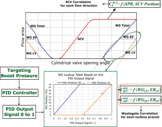
FIGURE 7. Methodology for simulating when the wastegate flow area is the same and when SCV is opened.

From Figure 7, it can be observed that, when the SCV is open totally, first the wastegate of the short volute is opened and then the long volute branch (as highlighted with a green circle). Similarly, a wastegate lookup is created to estimate the wastegate position of each branch. The lookup table is created based on the cylindrical valve information provided by the manufacturer, as shown in Figure 7. To decide the long and short volute wastegate positions in the simulation, a PID controller is employed, and it targets the experimental boost pressure value (p₂^′). The PID generates an output signal value from 0 to 1, and accordingly, the wastegate lookup is created. During the engine simulation, at every time step, the PID sends a signal (between 0 and 1) to the lookup table. Based on the value of the signal, the lookup table determines the wastegate position for short and long volutes. Finally, the wastegate position and the expansion ratio of the each branch at the current time step are passed to the wastegate correlation to calculate the discharge coefficients.

Regarding SCV, the tests were performed with totally opened valve position; therefore, the valve position is fixed to 100$\text{\%}$ during the entire simulation in all engine speeds. However, the SCV model depends on the scroll pressure ratio value, and it is different when the flow goes from branch to branch (i.e., LV to SV and SV to LV). Therefore, at every time step, the scroll pressure ratio across the SCV section is passed to the SCV correlation for estimating a discharge coefficient values for each flow direction. The designed control system continues until the PID reaches the target value (i.e., p₂^′), and all the other steady-state variables are converged. The working of this control system during the simulation is shown in Figure 8. The Figure 9 shows the GT-power model of the tested engine connected to the CMT-DETCM model. Also, the PID, orifice of SCV, and the wastegate of each branch and their correlations were highlighted, respectively.

FIGURE 8

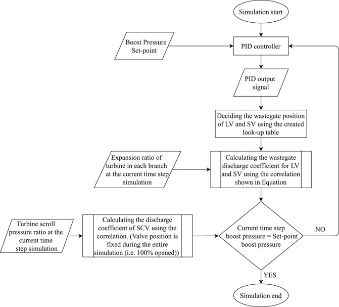
FIGURE 8. Working of the designed control system when the wastegate flow area is same and the SCV valve is opened.

FIGURE 9

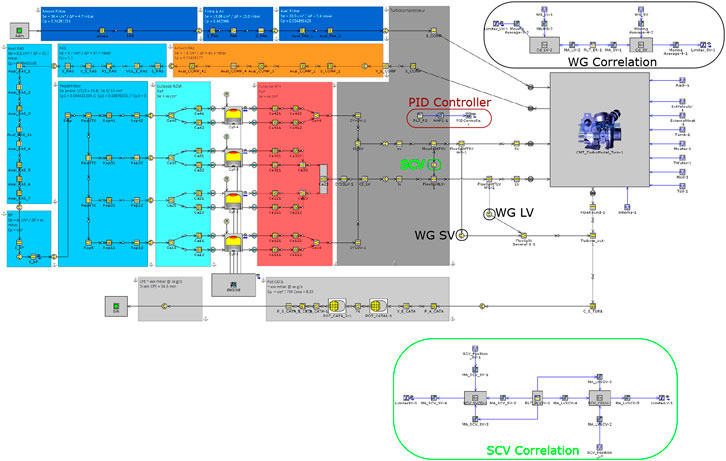
FIGURE 9. GT-power model of the tested engine and its connection to the dual-volute turbine model.

Full Load Points Simulation Results

Figure 10 shows the result of manifold boost pressure ($p_2^{\prime }$) in the engine simulations. It can be observed that the error between the experimental and model is very low. This confirms that the control design developed with the wastegate correlation is efficient enough to reach the target values. Figures 11A,B show the outcome of wastegate position and discharge coefficient values of each branch in engine simulation. It can be noted that the overall wastegate position values from the CMT-DETCM model are very close to the overall wastegate position obtained from the engine test cell, as shown in Figures 11A. These indicate that the turbine upstream pressure values in the simulation are also well predicted; the results are shown in following figures. From Figure 11A, one can notice that at low engine speed (1,250 rpm), the model indicates that the wastegate should be opened in order to reach the experimental boost pressure value. One possible reason could be small leakages from the cylindrical valve during the engine tests even when the wastegate is closed totally, and the discharge coefficient model is able to discover these leakages in the simulation.

FIGURE 10

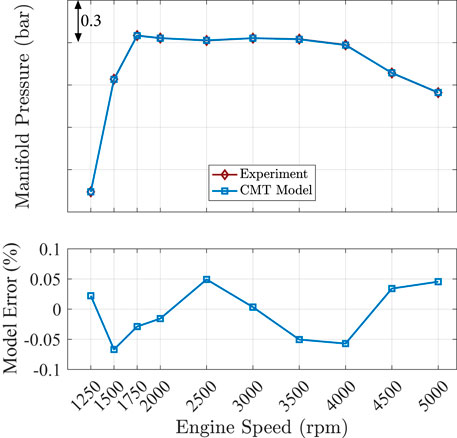
FIGURE 10. SCV opened inlet manifold boost pressure from the PID controller.

FIGURE 11

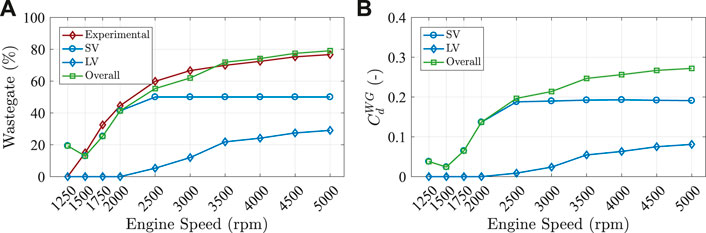
FIGURE 11. CMT-DETCM model wastegate positions and the estimated discharge coefficient values at different engine speeds.

Figure 12 shows the position of scroll connection valve and the estimated discharge coefficient values for each flow direction. Aforementioned, the SCV opened tests were performed with totally opened valve, and accordingly, in the simulation, the valve is fixed to 100% for all engine speeds as shown in Figure 12A. As discussed by Samala (2020), the flow passing from long to short and vice versa for the same operating point in the turbine is different. Due to the pressure drop across the SCV section is not the same in each flow direction. Consequently, the discharge coefficient values are different when the flow is moving from SV to LV and LV to SV in the simulations, as shown in Figure 12B.

FIGURE 12

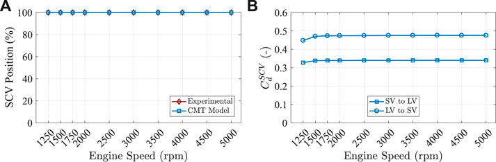
FIGURE 12. CMT-DETCM model SCV positions and the estimated discharge coefficient values at different engine speeds.

In order to compare the compressor and turbine performances, the turbocharger rotational speed has to be close to the experimental value. From Figure 13A, it can be seen that the simulated turbocharger speeds are not that far from the experimental results. Better predictions were observed at the low engine speeds, but at high engine speeds, the model is slightly underestimated. Nevertheless, the error from the model is not above $\pm$5% from the experimental value. The well predicted rotational speed highlights a reasonable estimation of friction losses and overall power balance. In the simulation, the wastegate position is changed until the manifold boost pressure ($p_2^{\prime }$) is achieved; therefore, compressor outlet temperature ($T_2$) will be the primary variable to validate the compressor performance and heat transfer. As it can be seen in Figure 13B, the model underestimates the compressor outlet temperature in all the engine speeds. However, the compressor outlet pressure from the model agrees well with the experimental points as shown in Figure 13C. So, the difference in the outlet temperature predictions is mainly related to the heat transfer problems. As stated in (Serrano et al., 2015a), the compressor outlet temperature ($T_2$) will be affected by the heat transfer for every operating condition and heat can be added or removed at the compressor outlet. Eventually, any temperature error from the compressor outlet is corrected by the WCAC heat transfer multipliers to be able to reach the inlet manifold temperatures. Figure 13D shows the results of the inlet manifold temperature compared to the experimental data, and it can be observed that the difference is always in between $\pm$5.2^∘C.

FIGURE 13

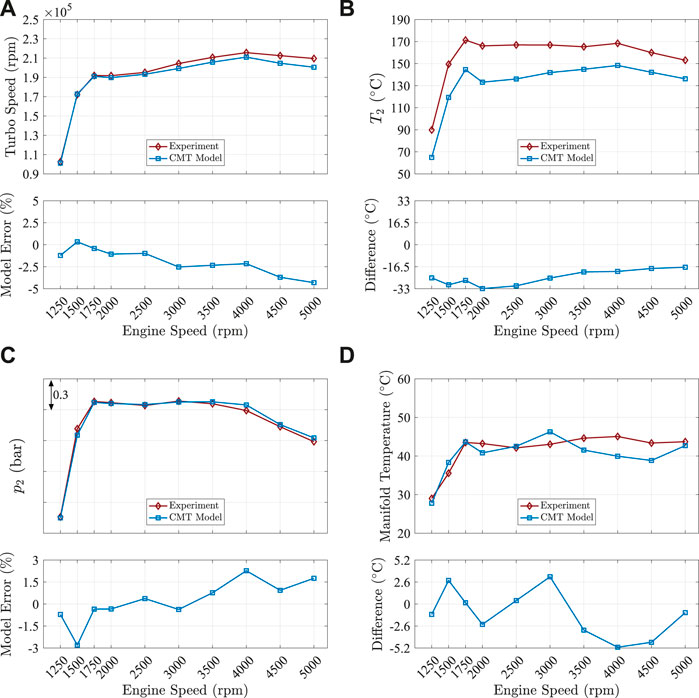
FIGURE 13. Validation parameters of SCV opened simulation. Outputs from the CMT-DETCM model compared against the experimental data at different engine speeds. (A) Turbocharger speed; (B) compressor outlet temperature; (C) compressor outlet pressure; (D) inlet manifold temperature.

Suppose the engine boundary conditions of the model are well fitted with the experiments that are inlet manifold (p₂^′) and exhaust manifold pressures ($p_{3,\text{LV/SV}}$). The air mass flow produced by the model should correspond to the experimental values. From Figure 14A, it can be observed that the air mass flow predictions are similar to the experimental results in the simulation. However, at engine speeds of 2,000 and 2,500 rpms, the relative error is above 5% and is more significant since the air mass flow lowers. This difference may be due to several engine-related slight uncertainties, including the blow-by air mass flow (which is not sensed by the air flow meter), the discharge coefficient of the intake valves, or the cylinder walls temperature during the intake stroke.The points with the low error indicate that the engine model is operating close to the experimental conditions. Figure 14B reveals the fact that if the model well predicts engine air mass flow, then the torque shows no significant mismatch against the experimental data. The small disagreement between the model and experimental torque values can come from the modelling of friction mean effective pressure (FMEP) and combustion. Figures 14C, D show the upstream turbine pressure in both long and short volute branches. It is evident that the mean pressure values with the CMT-DETCM model agree well with the experimental data in both turbine branches. These indicate that the backpressure from the turbine to the engine is also well captured. In order to check the accuracy of gas dynamics in the model, instantaneous turbine upstream pressure values are needed. However, from the engine tests, the instantaneous pressure data were not available due to the space difficulties of placing the instantaneous sensors at the turbine inlet.

FIGURE 14

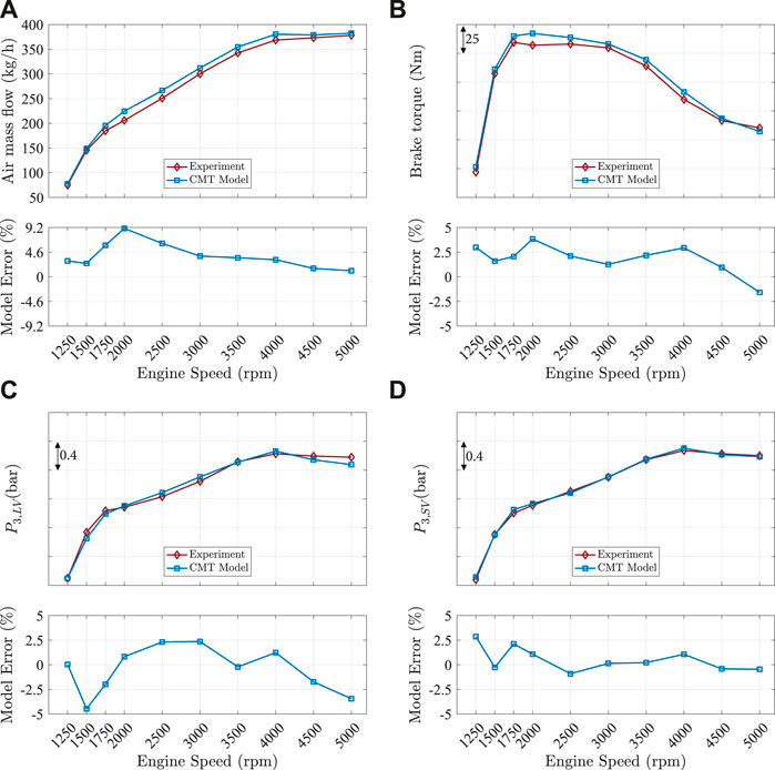
FIGURE 14. Validation parameters of SCV opened simulation. Outputs from the CMT-DETCM model compared against the experimental data at different engine speeds. (A) Air mass flow; (B) brake torque; (C) turbine inlet pressure in LV; (D) turbine inlet pressure in SV.

Figures 15A, B show the results of turbine inlet temperatures at long and short volute branches. The difference between the model estimated and experimental temperatures in the long volute branch at engine speeds are always in between $\pm$15^∘C. The few discrepancy in temperature predictions can be from the usage of exhaust heat transfer multiplier correlation that is found for single entry VGT/WG turbines. Figure 15B shows the results of temperatures in the short volute branch. Aforementioned, the temperature values for this branch from the experimental are reasonably lower when compared with the long volute temperature values. Nevertheless, the model shows the temperature levels in the short volute branch are similar to the long volute branch. The difference found between them from simulation is in the range of 30–40^∘C, which is a reasonable value as compared to the difference found in the experiments (Dale and Watson, 1986). Figures 15C, D show the results of temperature and pressure at the turbine outlet. The outlet temperatures from the model are slightly lower than the experimental values, and the difference is not greater than $\pm$50^∘C. This difference can be explained due to the effects of heat transfer problems in the double-entry turbines. Figure 15D shows after-treatment back-pressure to the turbine from both CMT-DETCM models, and they are in good agreement with the experimental values.

FIGURE 15

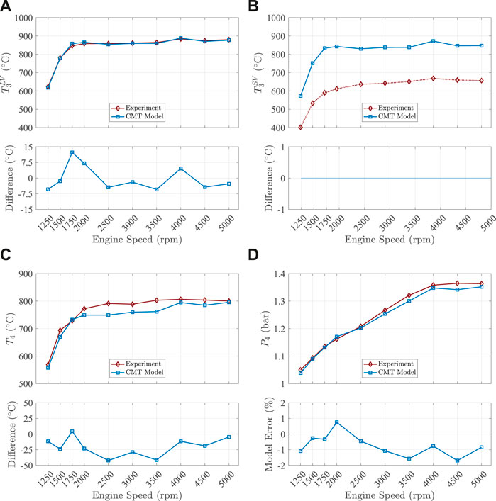
FIGURE 15. Validation parameters of SCV opened simulation. Outputs from the CMT-DETCM model compared against the experimental data at different engine speeds. (A) Turbine inlet temperature LV; (B) turbine inlet temperature SV; (C) turbine outlet temperature; (D) turbine outlet pressure.

In summary, the engine simulation with the described double-entry turbine models shows that in all validation parameters, the discrepancies between the model and experimental are reasonable. A good reproduction of turbine inlet pressure and temperature together with a well-estimated turbine outlet temperature indicates that the experimental running point and wastegate opening of the turbine has been correctly found inside turbine maps.

Results of Instantaneous Performance Parameters

In this section, the unsteady operation of the double-entry turbine parameters obtained from the simulation is compared with the different steady flow admission state performance parameters. The unsteady operation results are shown for engine speeds of 3,000 and 5,000 rpms.

Rapid fluctuations of the pressures at every inlets and outlet of turbine lead to an immediate alteration on turbine mass flow in each branch, as shown in Figure 16. It is worth highlighting that the instantaneous mass flow is extracted at the turbine tongue outlet (station A) as represented in Figure 1. Furthermore, the extracted mass flow values of each branch shown in Figure 16 are after subtracting the amount wastegate flow of that branch, respectively. To indicate flow admission conditions of the turbine at shown engine speeds, the mass flow ratio (MFR) is represented, and it is calculated as shown in the Eq. 1. From Figure 16, it can be perceived that the maximum mass flow in each branch is nonidentical. It is due to the different wastegate position of every branch, as shown in Figure 11A and Figure 8. For example, when the engine is working at 3,000 rpm (Figure 16A), wastegate of the short volute branch is opened to its maximum value. Whereas, in the case of a long volute branch, the wastegate is slightly opened. Due to this, there is a maximum flow in long volute branch than the short volute branch. From Figure 16, it can be observed that MFR is changing from 0.3 to 0.8 for an engine speed of 3,000 rpm. Even in the case of higher engine speed (5,000 rpm), the change in MFR is from 0.1 to 0.9. These conclude that the double-entry turbines always work in between full and unequal flow admission conditions with the engine, and it never approaches to the partial admission state (i.e., to MFR 0 or 1).

FIGURE 16

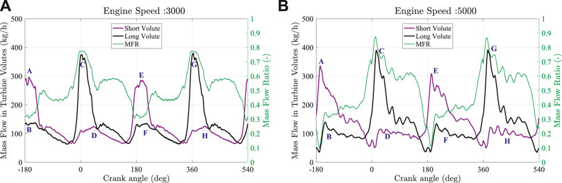
FIGURE 16. Engine instantaneous mass flow rate results from simulation in each turbine branch of the dual-volute turbine. (A) Simulation results of engine speed 3,000; (B) simulation results of engine speed 5,000.

Figure 17 shows the instantaneous traces of turbine reduced mass flow parameter and expansion ratio in each branch at engine speeds of 3,000 and 5,000 rpms. Instantaneous expansion ratio calculated by a model in each branch is considered between the turbine tongue outlet (station A) and turbine diffuser inlet (station F), as shown in Figure 1. Whereas, reduced mass flow is considered at turbine tongue outlet (station A). In order to compare the instantaneous traces, they are plotted with the different steady-state admission extrapolated curves (counters) of every branch obtained from the CMT-DETCM model (Samala, 2020). It should be noted that, when MFR is increasing, the mass flow conditions in the long volute branch increases and short volute branch decreases.

FIGURE 17

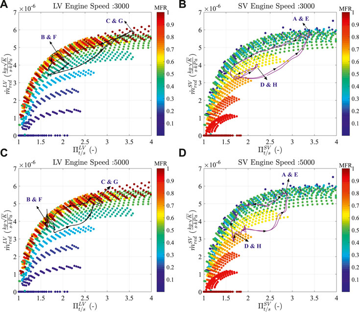
FIGURE 17. Comparison of steady (contours) and unsteady state reduced mass flow parameter vs. expansion ratio across each turbine branch obtained from the CMT-DETCM model. (A) and (B) Show the instantaneous parameters in long and short volute branches for an engine speed of 3,000 rpm; (B) and (D) show the instantaneous parameters in long and short volute branches for an engine speed of 5,000 rpm.

The first noticeable characteristic of the instantaneous trace is that a hysteresis loop is formed as the pressure rises and falls throughout the pulse energy coming from the engine. The rotation of the hysteresis loop occurred in an anticlockwise direction, as shown by the arrow in Figure 17. This loop implies the rate of change of reduced mass flow parameter will be different when the pressure is rising than when the pressure is falling in each turbine branch. Every point along the instantaneous trace (shown with black and purple lines in Figure 17) represents the flow conditions of the turbine, at an instance in time. As pointed out in Figure 17, the instantaneous traces exhibits a smaller, secondary loop (pointed with B and F in long volute; D and H in short volute) at the base of the trace where the expansion ratio is low in the idle period of a pulse (Figure 16). The secondary loop is caused by a small rise in pressure in the one branch when there is a pressure rise in the second branch (Figure 16). In other words, these small loops indicate that a rise in pressure due to the peak of pulse in the long volute branch (C and G in Figures 17A, C) can be felt in the short volute branch (D and H in Figures 17B, D). The same can be observed when there is a rise in pressure in the short volute branch (A and E in Figures 17B, D) and can be felt in the long volute branch (B and F in Figures 17A, C). This secondary loop is much more noticeable when the turbine is working with an engine speed of 3,000 rpm than with the 5,000 rpm engine speed. This is due to the highly different wastegate positions in each turbine branch when the turbine is working at engine speed of 3,000 rpm.

Figure 18 and Figure 19 show the comparison between the steady-state extrapolated turbine apparent and actual efficiencies (contours) with instantaneous apparent and actual turbine efficiency (black and purple lines actual) of each branch of the dual-volute turbine obtained from the simulation at 3,000 and 5,000 engine speeds. The CMT-DETCM model calculates the turbine efficiency and blade to speed ratio between the stator inlet and rotor outlet nozzles (stations C and E, respectively, in Figure 1).

FIGURE 18

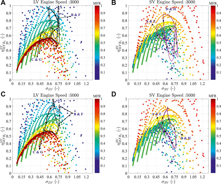
FIGURE 18. Comparison of steady (contours) and unsteady state parameters of total to static turbine efficiency (apparent efficiencies) with blade speed ratio across each turbine branch. (A) and (B) Show the instantaneous apparent efficiency values in long and short volute branches for an engine speed of 3,000 rpm; (B) and (D) show the instantaneous apparent efficiencies in long and short volute branches for an engine speed of 5,000 rpm.

FIGURE 19

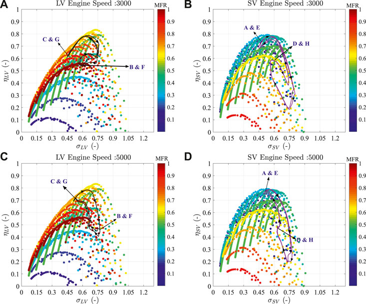
FIGURE 19. Comparison of steady (contours) and unsteady state parameters of total to static turbine efficiency (actual instantaneous efficiencies) vs. blade speed ratio across each turbine branch and for different MFR levels. (A) and (B) Show the instantaneous actual efficiency values in long and short volute branches for an engine speed of 3,000 rpm; (B) and (D) show the instantaneous actual efficiencies in long and short volute branches for an engine speed of 5,000 rpm.

The instantaneous apparent efficiency values in both long and short volute branches are shown in the Figure 18 for both engine speeds. It can be observed that the apparent efficiency values are changing with a great extent around the same blade speed ratio values in both branches. Furthermore, the steady-state extrapolated values (contours) from the CMT-DETCM model are also at 100$\text{\%}$ efficiency values when the MFR values are lower in long volute and higher in the short volute. It is worth highlighting that the apparent efficiency values are calculated with a mixture of turbine outlet temperatures coming from individual branches (Figure 20 (process shown with separated lines) and Eq. 3). Therefore, the apparent efficiency is not a good definition in the cases of very high and low unequal flow admissions to reflect which branch is extracting energy more efficiently from the flow upstream of the turbine. Just in the case of full (MFR 0.5) and partial admissions (MFR 0 and 1), the apparent efficiency representation signifies the energy extraction of every branch reasonably. Therefore, observing the apparent instantaneous efficiency trace, it can be said that the nonpulsating branch produces large efficiency due to the pulses generated in the other branch. In other words, the branch connected to an exhaust valve that is closed will show massive efficiency changes while it is mass flow drop.

FIGURE 20

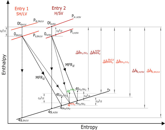
FIGURE 20. Enthalpy-entropy expansion process in twin-entry/dual-volute radial turbines, Serrano et al. (2020b).

It is worth highlighting that the double-entry turbine model described in (Serrano et al., 2020b) has the capability of estimating the actual turbine efficiencies of each branch (Eqs. 9 and 10). The model calculates the actual efficiencies in each branch using their respective turbine inlet and outlet conditions (as the process shown with continuous lines in Figure 20). Therefore, these efficiency values never be at 100$\text{\%}$ as shown in Figure 19. Furthermore, there will not be any massive changes, as seen in apparent efficiency values (Figure 18). These efficiency values will help taking better conclusions during the design phase and calibration process of the turbocharger and its correspondent engine. From Figure 19, it can be concluded that the actual efficiency values are very well represented with flow conditions in their respective turbine branches. For example, observing the instantaneous actual efficiency values in both branches for engine speed of 3,000 rpm (Figures 19A, B), two levels of oscillation of efficiency around optimum blade speed ratio (around 0.67) can be observed. One level associated to optimum MFR of around 0.6 and another associated with a maximum MFR of around 0.9.

Conclusion

In the current study, all models were integrated into the one-dimensional simulation software and were validated entirely by coupling them with the 1D calibrated engine model at full load curves obtained from the engine experimental campaign. The validation is performed only for the engine full load curves obtained when the both scroll connection valve and wastegate valve are opened. During the engine simulation, only one full and two partial admission maps obtained from the gas stand were used in the turbocharger model for the calibration.

The engine model was configured to converge on the experimental intake manifold pressure as a target for each engine speed by using the in-built turbocharger wastegate controller. The results from engine simulation were compared with the corresponding experimental data obtained from the engine test bench. The intake manifold pressure from the simulation confirms that the specified performance target was able to meet with the designed controller. The main findings of the simulations are that the engine brake torque and air mass flow were able to reach the experimental values with a maximum relative error of 4$\text{\%}$ and 9$\text{\%}$, respectively. Furthermore, comparison to the other measured engine test parameters such as intake manifold temperature, turbocharger speed, turbine upstream, and downstream pressures showed the satisfactory validation of the engine model with the described double-entry models in this paper.

Observing the instantaneous results from the simulation with steady-flow maps in each branch, they showed the importance of having the systematized performance maps for double-entry turbines as two individual turbines and modelling accordingly. Furthermore, it concludes that the turbine model is able to catch all the flow situations coming from the engine in each branch and is able to reproduce the engine performance similar to experimental values.

Annex

Double-Entry Turbine Models Description

Here, an overview of testing and modelling the double-entry turbines with different flow admission conditions is presented. The procedure for systematizing the performance maps of double-entry turbines and modelling methodology was described briefly, and more details about the method can be read at (Serrano et al., 2019c; 2020b). The double-entry turbine models have been validated previously using the different flow admission conditions in twin-entry and dual-volute turbine types Serrano et al. (2020b). The novelty of the model is its ability to be used in a quasisteady way for twin-entry and dual-volute turbines performance predictions. Furthermore, two discharge coefficient correlations were presented that were used in engine simulation: one for wastegate valve and another for scroll connection valve for estimating the discharge coefficients of the same in the 1D engine simulations.

Double-entry turbine testing method and maps characterization

In normal engine operating conditions, double-entry turbochargers (twin-entry or dual-volute) operate under different flow admission conditions due to the pulsating nature of exhaust gas coming from the engine cylinders. The flow admission conditions are further divided into three different categories as follows:

• Partial: when the flow is only in one of the turbine inlets while the other inlet is working with zero flow

• Equal/full: when the flow rate is the same in each branch of the turbine

• Unequal: when the flow, temperature, and pressure levels between the turbine branches are different. These are the cases at which the double-entry turbochargers operate in an engine most of the time.

The overall turbine performance will certainly depend on the mass flow distribution among each entry of the turbine. Therefore, to support the development of the mass flow parameter model and turbine efficiency model of double-entry turbines, a turbocharger test rig has been designed to test the turbine under a variety of steady flow admission conditions at the turbine inlets as discussed by Serrano et al. (2019c). One of the main advantages of this test rig is to be able to control and measure the mass flow rate in each turbine branch independently. Furthermore, the pressure and temperatures were also able to record in each branch. In order to test and classify the flow admission conditions mentioned above, Serrano et al. (2019c) suggested a parameter called MFR (mass flow ratio). The MFR parameter decides the amount of flow going into each branch, and it is defined as actual mass flow in long volute to the addition of actual flows in both branches as shown in the following equation:

$\text{MFR}=\frac{{\dot{m}}_{\text{Sh/LV}}}{{\dot{m}}_{\text{Sh/LV}}+{\dot{m}}_{H/\text{SV}}}.(1)$

The MFR definition with actual mass flows makes it simpler to test any double-entry turbine in a standard gas stand. Moreover, the MFR is proportional to the ratio of power in one branch to total turbine power. In every tested MFR, the total inlet mass flow is changed accordingly to obtain the same operating range and corrected speeds of the compressor. This way, both twin-entry and dual-volute turbines were characterized by employing different steady flow admission conditions. The main points of the test rig and the methodology for testing the double-entry turbines were demonstrated with the measurement uncertainty in an earlier work by Serrano et al. (2019c).

Representing the double-entry turbines flow performance maps as a single entry turbine, the mass flow distribution between respective branches under full and unequal admission conditions is not known. Furthermore, using the average values between the two branches such as the expansion ratio and turbine scroll temperature in calculating the reduced flow parameter for all admission conditions as described by Romagnoli et al. (2012) did show an impact on resulting maps and made it very difficult to analyse them. For this reason, Serrano et al. (2019c) proposed to treat each turbine branch as a separate turbine working in parallel. This way, the parameters such as expansion ratio, reduced mass flow, and reduced speed can be computed for each branch using their corresponding inlet conditions as shown in the following equation, where the term i represents the generic code for the turbine branch:

${\text{Π}}_{i,\left(0t,4\right)}=\frac{p_{0t,i}}{p_4};{\dot{m}}_{\text{red},i}=\frac{{\dot{m}}_i\cdot \sqrt{T_{0t,i}}}{p_{0t,i}};n_{\text{red},i}=\frac{n}{\sqrt{T_{0t,i}}}.(2)$

Whereas, for calculating the efficiency of each turbine branch, Serrano et al. (2019c) assumed that the power produced by each branch is different. Accordingly, the total-to-static turbine efficiency can be computed as two individual turbines, as shown in Eq. 3. This equation is expressed based on the enthalpy-entropy adiabatic expansion process of the turbine shown in Figure 20 (the process shown with separated lines). The efficiency determined using Eq. 3 is called as apparent efficiency because $T_{4t}^{{\text{MFR}}_x}$ is common for both branches. As the turbine outlet temperature measured in the gas stand is the mass averaged mixed temperature. Since the temperatures coming from individual branches are mixed at the turbine outlet station (Figure 20, a process shown in separated lines),

${\eta }_{{\text{MFR}}_x\left(t/s\right)}^i=\frac{T_{0t,i}-T_{4t}^{{\text{MFR}}_x}}{T_{0t,i}-T_{4s,i}},(3)$

$T_{4s,i}=T_{0t,i}\cdot {\left(\frac{1}{{\text{Π}}_{i,\left(0t,4\right)}}\right)}^{\left(\frac{\gamma -1}{\gamma }\right)}.(4)$

The blade speed ratio (σ) is also considered for each turbine branch, and it is computed as shown in the following equation:

${\sigma }_i=\frac{2\cdot \text{π}\cdot n\cdot r_3}{\sqrt{2\cdot c_{p,i}\cdot T_{0t,i}\cdot \left[1-{\left(\frac{1}{{\text{Π}}_{i,\left(0t,4\right)}}\right)}^{\frac{\gamma -1}{\gamma }}\right]}}.(5)$

The performance maps obtained using the method proposed by Serrano et al. (2019c) (as it is summarized above) provided reliable information of flow going into each turbine branch at different flow admission conditions as shown in Figure 21. In the figure, the mass flow and efficiency data are normalized by the maximum experimental values of every branch. Furthermore, the mass flow map of each branch can be linked to the apparent efficiency map of each branch. The systematized approach allows using current variable geometry turbine models as two separate turbines for extrapolating and interpolating the mass flow and apparent efficiency parameters to off-design conditions. In the following sections, a summary of how the variable geometry turbine models of Payri et al. (2012) and Serrano et al. (2016) are used and adapted for double-entry turbines is explained.

FIGURE 21

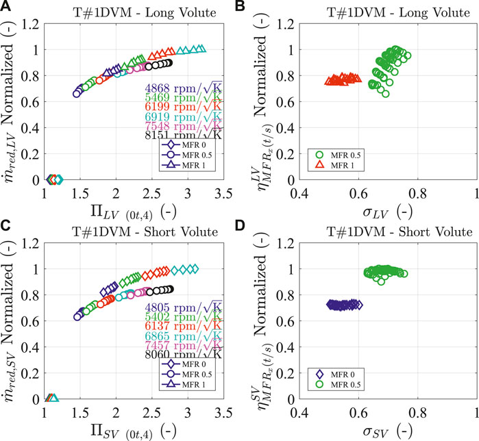
FIGURE 21. Turbine mass flow and apparent efficiency maps of dual-volute mixed flow turbine tested under full (MFR 0.5) and partial (MFR 0 and 1) flow admission conditions in the gas stand, Samala (2020).

Reduced Mass Flow Model

The turbine reduced mass flow parameter modelling is based on the VGT model described in (Serrano et al., 2016). It is suggested that the turbine can be modelled as an equivalent nozzle with an effective area which changes with respect to the flow conditions in the turbine. In the approach of considering each branch of double-entry turbines as a separate turbine, the resulting mass flow parameters showed a dependency of the flow behaviour with MFR as shown in Figure 21 and Serrano et al. (2019c). Therefore, Serrano et al. (2020b) redesigned the VGT turbine model to deal with dual-volute and twin-entry turbines.

The approach is based on viewing both branches as two separate parallel equivalent nozzles, as shown in Figure 22. This way, each equivalent nozzle has its respective set of flow map depending on the MFR instead of a VGT position. The value of the effective area of two nozzles is calculated in the same way as in the case of a single entry VGT turbine, that is using the individual flow performance maps shown in Figure 21 for each branch (i.e., for each equivalent nozzle).

FIGURE 22

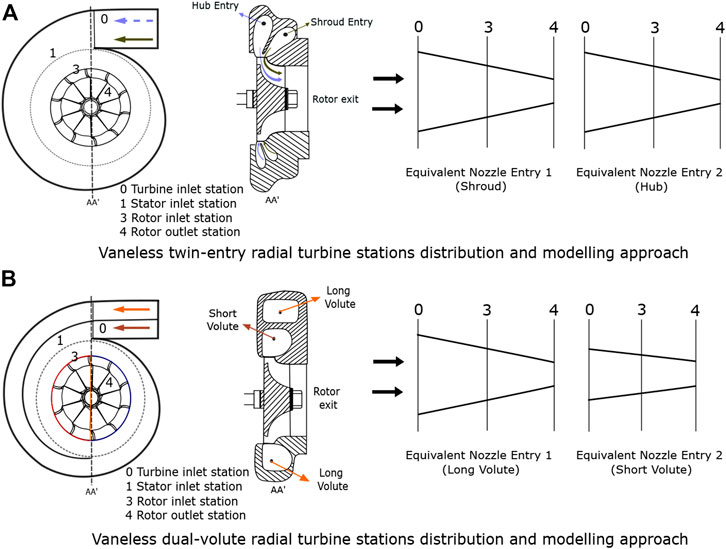
FIGURE 22. Vaneless double-entry turbines station distribution and two entries into two equivalent nozzles, Serrano et al. (2020b).

Eq. 6 shows the final expression of an effective equivalent nozzle area for each branch of the double-entry turbine. The terms i and j represent the generic codes for the turbine inlet (long volute or short volute; shroud or hub) and the double-entry turbine type (dual-volute or twin-entry) receptively. In summary, in each turbine type, there are two effective area equations (one for each turbine branch), which are dependent on their corresponding measured data of apparent efficiency (${\eta }_{MF{R}_x\left(t/s\right)}^i$), turbine entry geometries, and the four fitting constants ($a_i^j$, $b_i^j$, $c_i^j$, and $d_i^j$),

$A_{\text{eff},i}^j=\frac{a_i^j\cdot A_{4,i}^{j\text{geom}}\cdot \sqrt{1+\frac{{\left({\sigma }_i^j\right)}^2\cdot [{\left(\frac{D_{4m,i}^j}{D_3^j}\right)}^2-1]+b_i^j}{{\overline{\eta }}_{{\text{MFR}}_x\left(t/s\right)}^i}}}{\sqrt{1+{\left(c_i^j\cdot \frac{A_{4,i}^{j\text{geom}}}{A_{3,i}^{j\text{geom}}}\right)}^2\cdot \frac{{\left(\frac{1}{{\text{Π}}_{i\left(\mathrm{3,4}\right)}^j}\right)}^2}{\left(1-{\eta }_{{\text{MFR}}_x\left(t/s\right)}^i\cdot \left(1-{\left(\frac{1}{{\text{Π}}_{i\left(\mathrm{3,4}\right)}^j}\right)}^{\frac{\gamma -1}{\gamma }}\right)\right)2}}}.(6)$

Equation 6 also depends on stator and rotor outlet geometrical areas. It should be noted that the twin-entry and dual-volute turbines have different volute designs and geometries, and furthermore, they are vaneless turbines. Therefore, it is suggested that the stator and rotor outlet geometrical areas should be estimated in different ways for every turbine type. Moreover, in the approach of modelling the double-entry turbines as two separated equivalent nozzles, these areas are also defined precisely for each branch of every turbine type as discussed in Serrano et al. (2020b).

Once all the geometrical parameters are defined, the fitting is performed as two individual VGTs with their corresponding turbine entry map data. Serrano et al. (2020b) studied the behaviour of each coefficient of the effective equivalent nozzle area for both branches with every tested MFR. From the study, it was concluded that each coefficient showed a physical trend with the MFR in each branch. Later, it was reviewed how to impose those physical trends with MFR in each branch. It is concluded that the coefficient a can be imposed with a quadratic expression behaviour and other coefficients b, c, and d with a linear trend. This way, in global map fitting procedure, for both twin-entry and dual-volute turbines showed good results Serrano et al. (2020b). In summary, seven coefficients of each turbine branch can be adjusted using a nonlinear fitting method for all MFRs of a given branch at the same time. This implies that one single fitting procedure and one set of 7 coefficients will be needed for each turbine branch (in a total of 14 coefficients) to predict the effective equivalent nozzle area in all the admission conditions.

Once the effective equivalent nozzle area of each branch is known, the reduced mass flow parameter in each branch can be calculated using the expression of the flow through an orifice with an isentropic expansion, as shown in the following equation:

${\dot{m}}_{\text{red},i}^j=A_{\text{eff},i}^j\cdot \sqrt{\frac{\gamma }{R}}\cdot {\left(\frac{1}{{\text{Π}}_{i,\left(0t,4\right)}^j}\right)}^{\frac{1}{\gamma }}\cdot \sqrt{\frac{2}{\gamma -1}\cdot [1-{\left(\frac{1}{{\text{Π}}_{i,\left(0t,4\right)}^j}\right)}^{\frac{\gamma -1}{\gamma }}]}.(7)$

Adiabatic Efficiency Model

The procedure for the development of double-entry turbines efficiency was based on the VGT turbines efficiency model that is described in (Payri et al., 2012) and (Serrano et al., 2016). The VGT efficiency model is based on the use of Euler’s turbomachinery equation for radial gas turbines and assuming constant meridional component velocities. The purpose is to obtain an algebraic equation for the actual efficiency from a mean line analysis of the flow path in the turbine. With the hypothesis described in (Payri et al., 2012) and (Serrano et al., 2016), a final expression for estimating the efficiency maps for each VGT configuration has been developed. The final expression depends on the map data provided by the manufacturer, some geometrical information, and also with some fitting coefficients. The VGT efficiency has been redesigned for double-entry turbines in a similar way to the reduced mass flow fitting method; more details can be read in (Serrano et al., 2020b).

Aforementioned, the apparent efficiency of each turbine branch is defined as shown in Eq. 3, and Figure 20 (with the process shown in separated lines) is according to the assumption that each branch works like an individual turbine. Serrano et al. (2020b) investigated and concluded that the apparent efficiency could not be calculated directly using the final efficiency expression of the VGT turbine model. When the turbine is working under full and unequal admission conditions, at the rotor outlet, the temperature coming from the individual turbine branches may be different. These different temperatures will define the actual efficiency process shown with continuous lines in Figure 20, in contrast with apparent efficiency processes drawn with separated lines in Figure 20. The actual efficiencies of such continuous line processes, labelled as ${\text{MFR}}_x$ in Figure 20, are what could be calculated using the final efficiency expression of the VGT turbine model. Although directly using the efficiency maps of partial admission (MFR = 0 and MFR = 1) for full and unequal admissions may seem like a right approach. Serrano et al. (2020b) proved that it is a bad approximation, showing that the measured turbine outlet temperature at full and unequal admissions ($T_4^{MFRx}$ in Figure 20) cannot be calculated just from $T_{4,\text{Sh/LV}}$ and $T_{4,\mathit{H}\text{/SV}}$ obtained from partial admission efficiency maps. In other words, $T_4^{{\text{MFR}}_x}$ cannot be calculated by mass averaging the temperatures as shown in the following equation:

$T_4^{{\text{MFR}}_x}=T_{4,{\text{Sh}}_x/{\text{LV}}_x}^{\text{TE/DV}}\cdot {\text{MFR}}_x+T_{4,{\text{Sh}}_x/{\text{SV}}_x}^{\text{TE/DV}}\cdot \left(1-{\text{MFR}}_x\right).(8)$

Therefore, to model the apparent efficiencies of twin-entry/dual-volute turbine behaves like two independent turbines always operating at partial admission conditions, some interactions between both turbine branches have to be taken into account. In this regard, Serrano et al. (2020b) developed an apparent efficiency formulation for each branch, as shown in Eqs. 9, 10. A more comprehensive analysis and detailed discussion about the development of this apparent efficiency formulation can be found in an earlier work (Serrano et al., 2020b). It is worth noting that the final formulations showed in Eqs. 9, 10 are a function of actual efficiencies (not apparent), expansion ratios, and total inlet temperature of both turbine branches to follow the mixing approach and to obtain the apparent efficiency measured in the gas stand. The two equations are fitting together with 11 coefficients, and it uses the limited amount of data points from turbine maps of both branches and some geometrical informations.

$\begin{array}{c}{\eta }_{{\text{MFR}}_x\left(t/s\right)}^{{\text{Sh}}_x/{\text{LV}}_x}={\text{MFR}}_x\cdot {\eta }_{{\text{Sh}}_x/{\text{LV}}_x}^{\text{TE/DV}}+\frac{1-{\text{MFR}}_x}{\left(1-{\left({\text{Π}}_{0t,4}^{{\text{Sh}}_x{\text{LV}}_x}\right)}^{\frac{1-\gamma }{\gamma }}\right)}\\ \cdot \left[1+\left({\eta }_{H_x/{\text{SV}}_x}^{\text{TE/DV}}\left(1-{\left({\text{Π}}_{0t,4}^{H_x{\text{SV}}_x}\right)}^{\frac{1-\gamma }{\gamma }}\right)-1\right)\frac{T_{0t}^{H_x/{\text{SV}}_x}}{T_{0t}^{{\text{Sh}}_x/{\text{LV}}_x}}\right]\end{array}(9)$

$\begin{array}{c}{\eta }_{{\text{MFR}}_x\left(t/s\right)}^{H_x/{\text{SV}}_x}=\left(1-{\text{MFR}}_x\right)\cdot {\eta }_{H_x/{\text{SV}}_x}^{\text{TE/DV}}+\frac{{\text{MFR}}_x}{\left(1-{\left({\text{Π}}_{0t,4}^{H_x{\text{SV}}_x}\right)}^{\frac{1-\gamma }{\gamma }}\right)}\\ \cdot \left[1+\left({\eta }_{{\text{Sh}}_x/{\text{LV}}_x}^{\text{TE/DV}}\left(1-{\left({\text{Π}}_{0t,4}^{{\text{Sh}}_x{\text{LV}}_x}\right)}^{\frac{1-\gamma }{\gamma }}\right)-1\right)\frac{T_{0t}^{{\text{Sh}}_x/{\text{LV}}_x}}{T_{0t}^{H_x/{\text{SV}}_x}}\right].\end{array}(10)$

One of the main advantages of both reduced mass flow and apparent efficiency models described here is that it can be used for both twin-entry and dual-volute turbines, just by giving attention to the geometrical simplifications while fitting the turbine type (Serrano et al., 2020b). Furthermore, it is essential to have a standard turbine map of each branch measured in the adiabatic conditions and with at least two extreme flows (MFR 0 and 1) and also full admission flow (MFR 0.5). Only these three MFRs needed to fit the coefficients of both models and also for extrapolating into other MFRs and also into off-design conditions of performance maps in each branch.

Discharge Coefficient Models

Wastegate

For a wastegate turbocharger, in 1D engine calculations, a wastegate model is necessary to control the boost pressure and also to predict the upstream turbine pressure accurately (Guzzella et al., 2010). The wastegate models can be in the form of discharge coefficient (GT-Power, 2017). Therefore, for estimating the discharge coefficient of a wastegate in the engine calculations, an empirical model has been used. The procedure to develop this empirical model is discussed deeply for a twin-entry turbine by (Serrano et al., 2017), and the same has been applied to a dual-volute turbine. It is suggested that the turbine can be tested in full admission with two different tests, first by closing the wastegate valve mechanically and second with the different levels of openings. In these two different tests, it is required to ensure that the turbine inlet temperature, expansion ratio, and turbocharge speed are maintained similar. Furthermore, the back-pressure valves at the compressor side should be kept constant. This way, it will guarantee that the turbine operative conditions will be similar when the wastegate is closed and opened. In the end, by making the difference between the two tests, mass flow through the wastegate can be easily calculated from the experiments. Subsequently, the experimental discharge coefficient can be evaluated by doing the ratio between the actual to ideal wastegate flows. Then, it can be correlated as a function of expansion ratio and wastegate valve position Serrano et al. (2017). Eq. 11 shows the expression for estimating the discharge coefficient of a wastegate for a dual-volute turbine, and it depends on three fitting coefficients (a, b, and c) as shown in the following equation:

$C_d^{\text{modDV}}=a\cdot {\text{Π}}_{t/s}\left(\frac{\text{\%WG}}{100}\right)+b\cdot {\left(\frac{\text{\%WG}}{100}\right)}^2+c\cdot \text{tan}\left(\frac{\text{\%WG}}{100}\right).(11)$

Scroll Connection Valve

When a scroll connection valve is present in a turbine, the flow can communicate between the turbine branches before going into the rotor. The advantage of having this valve is that it will allow the dual-volute turbines to work as a single entry turbine. When the SCV is opened, the engine mass flow from the active cylinder is shared between the two volutes. Therefore, to communicate the flows between the turbine branches in 1D engine simulations, an SCV discharge coefficient model which is developed previously has been used (Samala, 2020). The development of this model is carried out similar to the wastegate characterization, that is, performing two different tests: one with the SCV open and another SCV closed. But, these two tests are performed with a partial admission map of each branch (MFR 0 and 1). Testing each turbine branch separately, it was easy to estimate the flow that is passing in each direction (i.e., from long to short and vice versa) (Samala, 2020). From the experimental results, it was concluded that the SCV flow in each direction is not equal for same SCV openings. It is because the pressure drop across the SCV segment is different when the SCV flow is going from long volute to short volute and vice versa. Based on this, two different discharge coefficients were correlated as a function of scroll pressure ratio (SPR) and SCV openings, as shown in Eq. 12 (index k refers to the direction of SCV flow). More detailed analysis for the development of this correlation can be found in (Samala, 2020). The correlation is depended on six coefficients (a, b, c, d, e, and f). It should be noted that when the SCV flow is passing from long to short volute, the SPR is calculated using Eq. 13 and in the other flow direction using Eq. 14,

$C_{d,\text{mod}}^{\text{SCV},k}=a+\left[b\cdot \left(\text{sin}{\left(c\cdot \left(\frac{\text{\%SCV},k}{100}\right)+d\right)}^2\right)\right]+\text{exp}(e\cdot {({\text{Π}}_{\left(ts\right),k}^{\text{SPR}}-1)}^f),(12)$

${\text{Π}}_{\left(t/s\right)\text{LV}\to \text{SV}}^{\text{SPR}}=\frac{p_{03,\text{LV}}}{p_{3,\text{SV}}},(13)$

${\text{Π}}_{\left(t/s\right)\text{LV}\leftarrow \text{SV}}^{\text{SPR}}=\frac{p_{03,\text{SV}}}{p_{3,\text{LV}}}.(14)$

Mechanical Losses Model

Mechanical losses models developed by Serrano et al. (2013) are being studied into two different parts (${\dot{W}}_m={\dot{W}}_{jb}+{\dot{W}}_{tb}$) in accordance with turbocharger geometrical characteristics. The bearings are studied with the simplified geometry, and their behaviour is analysed by solving the Navier–Stokes equations and some simplifying assumptions. Oil behaviour is considered incompressible, and its flow through the bearing is deemed to be steady and constant on each section. Also, circumferentially symmetric. Furthermore, the body forces are neglected, and the film thickness is considered smaller than any other bearing part. Viscous stresses are considered comparable to the inertial forces of the fluid (small Reynolds number: $Re=\rho u_c/\mu$).

Solving Navier–Stokes equations in the journal bearing with those simplifying assumption, the corresponding friction losses are expressed by Eq. 15. As it is observed, those losses depend on shaft rotational speed (N), oil viscosity (μ) at the average oil temperature (${\overline{T}}_{oil}$), geometrical parameters such as journal bearing radius ($R_{jb}$) and bearing length ($L_{jb}$), oil film thickness ($h_{jb}$), and a fitting parameter $k_{jb}$,

${\dot{W}}_{\text{jb}}=2\pi R_{\text{jb}}^3{k}_{\text{jb}}\frac{L_{\text{jb}}}{h_{\text{jb}}}{N}^2\mu \left({\overline{T}}_{\text{oil}}\right).(15)$

To the same extent, in the thrust bearing, friction losses may be expressed by Eq. 16, where $k_{tb}$ is a fitting factor, $R_{\text{tb,max}},R_{\text{tb,min}}$, and ${\overline{R}}_{\text{tb}}$ are the maximum, minimum, and average radius of Figure 23, φ is a geometrical parameter defined by Eq. 17, and $k_m$ denotes the fraction of lubricating oil passing through the considered bearing. Finally, $F_{at}$ is a term accounting the forces acting on the thrust bearing due to compressor and turbine pressure ratios difference. It is expressed by Eq. 18, referring to Figure 24, where $p_2^{\prime }$ and $p_3^{\prime }$ are the pressures at the outlet of the compressor wheel and the inlet of the turbine wheel, respectively, and in the previous equations, $A_{\text{comp}}^{\prime }$ and $A_{\text{turb}}^{\prime }$ are the effective areas of the compressor and turbine wheels,

${\dot{W}}_{\text{tb}}=k_{\text{tb}}\pi \left(R_{\text{tb,max}}^2-R_{\text{tb,min}}^2\right){\overline{R}}_{\text{tb}}^2\sqrt[3]{\left|\frac{F_{\text{at}\rho }}{12k_m\dot{m}\phi \mu \left({\overline{T}}_{\text{oil}}\right)}\right|}{N}^2\mu \left({\overline{T}}_{\text{oil}}\right),(16)$

$\phi =\frac{R_{\text{tb,max}}^2[log\left(R_{\text{tb,max}}\right)-0.5]}{2}-\frac{R_{\text{tb,min}}^2[log\left(R_{\text{tb,min}}\right)-0.5]}{2},(17)$

$F_{\text{at}}=\left|A_{\text{comp}}^{\prime }\frac{p_1-p_2}{4}-A_{\text{turb}}^{\prime }\frac{p_3^{\prime }-p_4}{2}\right|.(18)$

FIGURE 23

FIGURE 23. Simplified schemes of a journal bearings (left) and a thrust bearing (right), Serrano et al. (2013).

FIGURE 24

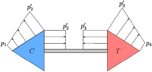
FIGURE 24. Schematic pressure distribution at the compressor and turbine wheels, Serrano et al. (2013).

Data Availability Statement

The raw data supporting the conclusions of this article will be made available by the authors, without undue reservation.

Author Contributions

JS, JG, and VS proposed the idea, conceptualization and performed data analysis; JM and VS performed experimentation and VS performed the modelling work under the supervision of JS, and JG; VS and JS prepared the original draft. Further, all authors have contributed to the revision and organization of the paper. All authors have read and agreed to the published version of the manuscript.

Funding

VS was partially supported through post-doctoral contract 2020-UPV-SUB.2-12450 of Science, Technology and Innovation in research structures of Universitat Politécnica de-Valéncia (UPV).

Conflict of Interest

The authors declare that the research was conducted in the absence of any commercial or financial relationships that could be construed as a potential conflict of interest.

Nomenclature

A Area (m)

a Rotor discharge coefficient (-)

b Reduced mass flow fitting coefficient (-)

BEVs Battery electric vehicles (-)

BSR Blade speed ratio (-)

c Reduced mass flow fitting coefficient (-)

$c_p$ Specific heat capacity (J kg⁻¹ K⁻¹)

$C_D$ Discharge coefficient (-)

$\text{DV}$ Dual-volute (-)

EGR Exhaust gas recirculation (-)

$\text{LV}$ Long volute (-)

$\dot{m}$ Mass flow (kg/s)

$\text{MFR}$ Mass flow ratio (-)

n Rotational speed (rpm)

p Pressure (Pa)

r Rotor radius (m)

$\text{Sh}$ Shroud (-)

$\text{SV}$ Short volute (-)

$\text{SPR}$ Scroll pressure ratio (-)

SCV Scroll connection valve (-)

T Temperature (K)

$\text{TE}$ Twin-entry (-)

VGT Variable geometry turbine (-)

VNT Variable nozzle turbine (-)

WG Wastegate (-)

$\text{Δ}{h}_{{\text{MFR}}_x}^{\text{Sh/LV}}$ Apparent work Entry 1

$\text{Δ}{h}_{{\text{MFR}}_x}^{\text{H/SV}}$ Apparent work Entry 2

$\text{Δ}{h}_{{\text{Sh}}_x/{\text{LV}}_x}$ Actual work Entry 1

$\text{Δ}{h}_{H_x/{\text{SV}}_x}$ Actual work Entry 2

$\text{Δ}{h}_{S,{\text{Sh}}_x/{\text{LV}}_x}$ Isentropic work Entry 1

$\text{Δ}{h}_{S,H_x/{\text{SV}}_x}$ Isentropic work Entry 2

Subscripts and Superscript

0t Turbine inlet total states

2 Compressor outlet static states

4 Turbine outlet static states

4s Turbine isentropic state

4t Turbine outlet total states

eff Effective equivalent nozzle

geom Geometry

i Discriminates $\text{Sh}$ from H in $\text{TE}$ or $\text{LV}$ from $\text{SV}$ in $\text{DV}$

j Refers to $\text{TE}$ or to $\text{DV}$ turbine

mod Model

red Refers to reduced variables

$t/s$ Total to static

Greek letters

η Corresponding efficiency

γ Heat capacity ratio

σ Corresponding blade speed ratio.

References

Costall, A. W., McDavid, R. M., Martinez-Botas, R. F., and Baines, N. C. (2010). Pulse performance modeling of a twin entry turbocharger turbine under full and unequal admission. J. Turbomach. 133. doi:10.1115/1.4000566.021005

CrossRef Full Text | Google Scholar

Dale, A., and Watson, N. (1986). Vaneless radial turbocharger turbine performance. In Proceedings of the IMechE. 65–76.

CrossRef Full Text | Google Scholar

Ding, Z., Zhuge, W., Zhang, Y., Chen, H., Martinez-Botas, R., and Yang, M. (2017). A one-dimensional unsteady performance model for turbocharger turbines. Energy 132, 341 – 355. doi:10.1016/j.energy.2017.04.154

CrossRef Full Text | Google Scholar

Galindo, J., Navarro, R., García-Cuevas, L. M., Tarí, D., Tartoussi, H., and Guilain, S. (2019). A zonal approach for estimating pressure ratio at compressor extreme off-design conditions. Int. J. Engine Res. 20, 393–404. doi:10.1177/1468087418754899

CrossRef Full Text | Google Scholar

GT-Power (2017). Gamma Technologies - Engine and Vehicle simulation manual. Available at: http://www.gtisoft.com.

Guzzella, L., Onder, C. H., Guzzella, L., and Onder, C. H. (2010). Introduction to modeling and control of internal combustion engine systems. Berlin, Germany: Springer, 1–20. doi:10.1007/978-3-642-10775-7

CrossRef Full Text | Google Scholar

Haq, G., and Weiss, M. (2016). CO2 labelling of passenger cars in Europe: status, challenges, and future prospects. Energy Policy 95, 324–335. doi:10.1016/j.enpol.2016.04.043

CrossRef Full Text | Google Scholar

Heywood, J., MacKenzie, D., Akerlind, I. B., Bastani, P., Berry, I., Bhatt, K., et al. (2015). On the road toward 2050: potential for substantial reductions in light-duty vehicle energy use and greenhouse gas emissions. Available at:http://web.mit.edu/sloan-auto-lab/research/beforeh2/files/On-the-Road-toward-2050.pdf

CrossRef Full Text | Google Scholar

Kalghatgi, G. (2018). Is it really the end of internal combustion engines and petroleum in transport? Appl. Energy 225, 965 – 974. doi:10.1016/j.apenergy.2018.05.076

CrossRef Full Text | Google Scholar

Martin, G., Talon, V., Higelin, P., Charlet, A., and Caillol, C. (2009). Implementing turbomachinery physics into data map-based turbocharger models. SAE Int. J. Engines 2, 211–229. doi:10.4271/2009-01-0310

CrossRef Full Text | Google Scholar

Martin, J., Arnau, F., Piqueras, P., and Auñon, A. (2018). Development of an integrated virtual engine model to simulate new standard testing cycles. SAE international, SAE technical papers, doi:10.4271/2018-01-1413

CrossRef Full Text | Google Scholar

Payri, F., Olmeda, P., Arnau, F. J., Dombrovsky, A., and Smith, L. (2014). External heat losses in small turbochargers: model and experiments. Energy 71, 534–546. doi:10.1016/j.energy.2014.04.096

CrossRef Full Text | Google Scholar

Payri, F., Serrano, J. R., Fajardo, P., Reyes-Belmonte, M. A., and Gozalbo-Belles, R. (2012). A physically based methodology to extrapolate performance maps of radial turbines. Energy Convers. Manag. 55, 149–163. doi:10.1016/j.enconman.2011.11.003

CrossRef Full Text | Google Scholar

Pla, B., la Morena, J. D., Bares, P., and Jiménez, I. (2020). Cycle-to-cycle combustion variability modelling in spark ignited engines for control purposes. Int. J. Engine Res. 21, 1398–1411. doi:10.1177/1468087419885754

CrossRef Full Text | Google Scholar

Rajoo, S., Romagnoli, A., and Martinez-Botas, R. F. (2012). Unsteady performance analysis of a twin-entry variable geometry turbocharger turbine. Energy 38, 176–189. doi:10.1016/j.energy.2011.12.017

CrossRef Full Text | Google Scholar

Romagnoli, A., Copeland, C. D., Martinez-Botas, R. F., Seiler, M., Rajoo, S., and Costall, A. (2012). Comparison between the steady performance of double-entry and twin-entry turbocharger turbines. J. Turbomach. 135. doi:10.1115/1.4006566

CrossRef Full Text | Google Scholar

Romare, M., and Dahllöf, L. (2017). The life cycle energy consumption and greenhouse gas emissions from lithium-ion batteries. IVL Swedish Environmental Research Institute 842, 978–991.

CrossRef Full Text | Google Scholar

Samala, V. (2020). Experimental characterization and mean line modelling of twin-entry and dual-volute turbines working under different admission conditions with steady flow. Ph.D. thesis, Valencia, Spain: Universitat Politècnica de València.

CrossRef Full Text | Google Scholar

Serrano, J., Arnau, F., Dolz, V., Tiseira, A., and Cervelló, C. (2008). A model of turbocharger radial turbines appropriate to be used in zero- and one-dimensional gas dynamics codes for internal combustion engines modelling. Energy Convers. Manag. 49, 3729–3745. doi:10.1016/j.enconman.2008.06.031

CrossRef Full Text | Google Scholar

Serrano, J. R., Arnau, F., De La Morena, J., Alejandro, G., Stephane, G., and Samuel, B. (2020a). “A methodology to calibrate gas-dynamic models of turbocharged petrol engines with variable geometry turbines and with focus on dynamics prediction during tip-in load transient tests.” in ASME turbo expo 2020, London, England.

CrossRef Full Text | Google Scholar

Serrano, J. R., Arnau, F., Garcia-Cuevas, L. M., Soler, P., Smith, L., Cheung, R., et al. (2019a). An experimental method to test twin and double entry automotive turbines in realistic engine pulse conditions. SAE International, SAE technical paper

CrossRef Full Text | Google Scholar

Serrano, J. R., Arnau, F. J., Andrés, T., and Samala, V. (2017). Experimental procedure for the characterization of turbocharger’s waste-gate discharge coefficient. Adv. Mech. Eng. 9, 168781401772824. doi:10.1177/1687814017728242

CrossRef Full Text | Google Scholar

Serrano, J. R., Arnau, F. J., Garcéa-Cuevas, L. M., Soler, P., and Cheung, R. (2019b). Experimental validation of a one-dimensional twin-entry radial turbine model under non-linear pulse conditions. Int. J. Engine Res. doi:10.1177/1468087419869157

CrossRef Full Text | Google Scholar

Serrano, J. R., Arnau, F. J., García-Cuevas, L. M., Dombrovsky, A., and Tartoussi, H. (2016). Development and validation of a radial turbine efficiency and mass flow model at design and off-design conditions. Energy Convers. Manag. 128, 281–293. doi:10.1016/j.enconman.2016.09.032

CrossRef Full Text | Google Scholar

Serrano, J. R., Arnau, F. J., García-Cuevas, L. M., and Samala, V. (2020b). A robust adiabatic model for a quasi-steady prediction of far-off non-measured performance in vaneless twin-entry or dual-volute radial turbines. Appl. Sci. 10, 1955. doi:10.3390/app10061955

CrossRef Full Text | Google Scholar

Serrano, J. R., Arnau, F. J., Gracía-Cuevas, L. M., Samala, V., and Smith, L. (2019c). Experimental approach for the characterization and performance analysis of twin entry radial-inflow turbines in a gas stand and with different flow admission conditions. Appl. Therm. Eng. 159, 113737. doi:10.1016/J.APPLTHERMALENG.2019.113737

CrossRef Full Text | Google Scholar

Serrano, J. R., Olmeda, P., Arnau, F. J., Dombrovsky, A., and Smith, L. (2015a). Turbocharger heat transfer and mechanical losses influence in predicting engines performance by using one-dimensional simulation codes. Energy 86, 204–218. doi:10.1016/j.energy.2015.03.130

CrossRef Full Text | Google Scholar

Serrano, J. R., Olmeda, P., Arnau, F. J., Reyes-Belmonte, M. A., and Tartoussi, H. (2015b). A study on the internal convection in small turbochargers. proposal of heat transfer convective coefficients. Appl. Therm. Eng. 89, 587–599. doi:10.1016/j.applthermaleng.2015.06.053

CrossRef Full Text | Google Scholar

Serrano, J. R., Olmeda, P., Tiseira, A., Garcéa-Cuevas, L. M., and Lefebvre, A. (2013). Theoretical and experimental study of mechanical losses in automotive turbochargers. Energy 55, 888–898. doi:10.1016/j.energy.2013.04.042

CrossRef Full Text | Google Scholar

Soler Blanco, P. (2020). Simulation and modelling of the performance of radial turbochargers under unsteady flow. Ph.D. thesis, Valencia (Spain): Universitat Politècnica de València

CrossRef Full Text | Google Scholar

Walkingshaw, J., Iosifidis, G., Scheuermann, T., Filsinger, D., and Ikeya, N. (2015). “A comparison of a mono, twin and double scroll turbine for automotive applications.” in ASME Turbo Expo 2015: Turbine Technical Conference and Exposition, Quebec, Canada, June 15–19, 2015

CrossRef Full Text | Google Scholar

Wang, S., Zhao, F., Liu, Z., and Hao, H. (2017). Heuristic method for automakers’ technological strategy making towards fuel economy regulations based on genetic algorithm: a China’s case under corporate average fuel consumption regulation. Appl. Energy 204, 544–559. doi:10.1016/j.apenergy.2017.07.076

CrossRef Full Text | Google Scholar

Wei, J., Xue, Y., Deng, K., Yang, M., and Liu, Y. (2020). A direct comparison of unsteady influence of turbine with twin-entry and single-entry scroll on performance of internal combustion engine. Energy 212, 118638. doi:10.1016/j.energy.2020.118638

CrossRef Full Text | Google Scholar

Zhu, D., and Zheng, X. (2017). Asymmetric twin-scroll turbocharging in diesel engines for energy and emission improvement. Energy 141, 702–714. doi:10.1016/j.energy.2017.07.173

CrossRef Full Text | Google Scholar