 Andrea Di Matteo
 Hesheng Bao
 Bart Somers
- Power & Flow Group, Mechanical Engineering, Eindhoven University of Technology, Eindhoven, Netherlands
In this study, two different diesel-like igniting sprays are investigated: Engine Combustion Network (ECN) Spray C and D. In particular, this study focuses on the respective performances of the RANS and LES models to predict a turbulent, igniting spray using the OpenFOAM platform. The breakup model, discretization schemes, and case setups, including the combustion model, are kept constant in order to mitigate any potential effect on the simulation apart from intrinsic differences due to turbulence modeling. A classic κ-ε model is applied for the RANS approach, while a dynamic structure model is used to solve the momentum equation in the LES approach. The κ-ε model constants are tuned to obtain a suitable prediction of inert experiments. Both approaches exhibit a reasonable agreement with the inert experiments regarding the global spray characteristics, the liquid length, and the vapor penetration. However, the transient local properties, including the spatial distribution of mixture fraction variance and the species distributions, are not identical. For reacting conditions, the Flamelet Generate Manifold (FGM) model is adopted in both the LES and RANS simulations, using several enthalpy levels as the fourth dimension in the tabulation to account for local heat loss. The results show good agreement between the two turbulence models, in terms of liquid length, vapor penetration, and lift-off length, while a short ignition delay is registered for both sprays and turbulence frameworks. Turbulence–chemistry interaction (TCI) is considered by applying a presumed probability density function (β-PDF) to the mixture fraction, and is found to play a key role in the reproduction of species distribution in the domain.
Introduction
Emission regulations have become increasingly strict in recent years. Climate change is driving clients and companies to focus on reducing pollutant emissions. This is also true for the transport sector, where for a long time and for a long time to come, the internal combustion engine has been the primary source of propulsion. Over the past 20 years, emission regulations have evolved to such levels that the study of each minute detail is necessary in order to comply with regulations. In this respect, Computational Fluid Dynamics has become pivotal. However, several complexities arise in engine simulations, including turbulent flows in moving geometries, high pressure liquid injection (two phase flow), and chemical reactions (combustion), making it difficult to independently assess the quality of all sub-models.
For turbulent flow simulations of practical systems, a two model approach prevails, using a time averaging approach (Reynolds Averaged Navier-Stokes, RANS) and a spatial filtered approach (Large Eddy Simulation, LES). Each of these methods has its own advantages and disadvantages: RANS is extremely fast and widely used for industrial purposes; however, it is time averaged, meaning that the instant solution is not shown and therefore it is not precise enough to determine the relevant processes involved. LES is more precise, solving above a determined filter size and modeling everything below; however, it is computationally more expensive. Another level of simplification pertains to the choice of models that represent several physical processes occurring during injection and combustion, such as the spray breakup model, the evaporation model, and the combustion model itself. The latter model can be quite detailed; either all species are solved on runtime together with the turbulent flow or the solutions for both the combustion and turbulent flows are separated: the so-called tabulated model. The method used in this study is the Flamelet Generated Manifold (FGM) approach (Oijen van 2002), which is a tabulation method. This model simulates combustion for a canonical configuration (counterflow- and premixed-flame) and the results, in terms of controlled variables (primarily the mixture fraction and a progress variable), are stored in tables (manifolds) and are retrieved on runtime during the flow simulation. This way, only the transport equations for the chosen controlling variables are added to the simulation, instead of the equations for all species, significantly reducing the computational cost. The FGM model is based on the flamelet assumption (Peters, 1984): turbulent flame structures can be locally described by laminar flames. This assumption is widely adopted in spray combustion and more generally in engine combustion since the conditions for its validity are often verified in all types of internal combustion engines (excluding extremely high regimes). To be precise, the chemical timescale must be significantly smaller than the turbulent timescale; in other words, the flamelet can instantaneously adapt to the turbulent flow-field. Hence, a turbulent 3D flame can be decomposed and studied as an ensemble of 1D flames which can be simulated beforehand and the results of which are stored in tables. The turbulent-chemistry interactions are accounted for by using a presumed probability density function (PDF), applied to all the controlling variables. Several previous studies suggest that, depending on the case, neglecting the turbulent-chemistry interaction (TCI) may lead to flawed predictions during the combustion process (Pei et al., 2016; Bhattacharjee and Haworth, 2013; Desantes et al., 2020; Dahms et al., 2017).
Given the aforementioned assumptions in modeling the flow, injection, and combustion, a proper validation of full-engine simulations is of utmost importance. However, obtaining high-quality and high-resolution engine data is difficult. For this reason, a constant volume chamber is widely used to assess the quality of the CFD models. In this study, the so-called Spray C and Spray D introduced by the Engine Combustion Network (ECN) (ECN, 2022) are examined. The ECN is an international collaboration between several universities, institutes, and companies examining engine combustion. The collaboration aims to gather experimental data to provide a solid and complete characterization of the combustion process so that improvements in predictive CFD can be achieved. The most widely-studied setup is known as Spray A: a well-defined single orifice spray, injected into an ambient atmosphere with a temperature, pressure, and oxygen concentration closely resembling those found in diesel engines. An extensive database is available for inert and reacting conditions, detailing the liquid and vapor penetration, spatial fuel distribution (Pickett et al., 2011), ignition delay and lift-off length (Higgins and Siebers, 2001), and major species distribution (Maes et al., 2016; García-Oliver et al., 2017). In recent years, new single-hole nozzles with larger diameters were introduced, similar to those used in heavy-duty vehicle engines: Spray C and Spray D analyzed in this study. Both possess approximately the same diameter but differ in their proneness to cavitation. This phenomenon occurs when the local liquid pressure inside a nozzle (in general inside a tube) drops to a value that is lower than the liquid’s vapor pressure, leading to a change in phase and thus a restricted fluid vein. Cavitation directly affects injection, generally increasing the spreading angle and modifying the ignition behavior and emissions (Pickett et al., 2011; Pastor et al., 2018; Westlye et al., 2016; García-Oliver et al., 2020). Spray C is designed to enhance cavitation, whereas Spray D uses a converging nozzle to avoid this phenomenon. This difference leads to distinct flow developments outside the nozzles; the reason spray C and D were chosen in this study.
The primary objectives of this study are: 1) to demonstrate that the FGM model can effectively represent the experimental data; 2) to evaluate any differences between the RANS and LES frameworks; 3) to analyze any differences in the combustion parameters for Spray C and Spray D; and 4) to outline the model parameters used and the reasons behind them.
This paper is divided into various sections: the Model Details section describes the combustion and breakup models applied and the relevant equations for both. An overview of the computational domain is also provided. This is followed by a section where inert cases are validated. Finally, the reacting cases are analyzed, and the results for both turbulent frameworks are compared to the experimental database.
Model Details
In the following equations, the tilde (
FGM combustion model
As stated in the Introduction, the primary goal of this study is to assess the FGM combustion model using RANS and LES modeling to reproduce the spray behavior in the well-known benchmark cases Spray C and Spray D. The FGM model is a tabulated chemistry reduction approach that retrieves the relevant thermophysical properties from a pre-computed flamelet database, created beforehand by simulating physical-space laminar flames using the CHEM1D software (Somers LMT, 1994). In this study, the chemical mechanism comprising 54 species and 269 reactions (Yao et al., 2017) is adopted. In the FGM, the flame properties are stored in a database, parametrized by controlling variables, for which transport equations are solved in the 3D simulation. Subsequently, the solver, solving for the values of the controlling variables, directly applies the retrieved thermochemical properties. In general, for igniting FGM, the mixture fraction, Z, and a reaction progress variable, Yc, are used as controlling variables. In this case, the mixture fraction in the flamelet simulation is defined by Bilger’s approximation (Bilger et al., 1990) and its transport equation in turbulence is expressed as follows :
Here,
Species are chosen to ensure that
where
Both equations contain the term
where
where
This type of sub-grid modeling is called a dynamic structure model; for further details, please refer to Bharadwaj et al. (2009), Tsang et al. (2019), and Bao et al. (2022).
In this work, the combustion model library is extended by adding the mixture fraction variance and the enthalpy. The former is added so that the turbulence–chemistry interaction is included, representing the influence of turbulence on combustion. Neglecting this effect would not only produce different distributions and species concentration peaks in the simulation (higher
where the shape parameters,
In order to apply this to the mixture fraction, a transport equation for
where
where
In this study, enthalpy was added as an extra controlling variable in order to describe the effect of spray evaporation; the enthalpy departs from a pure adiabatic mixing line that would occur if two gases with different temperatures would mix. The implementation of this additional control variable leads to FGM tables with different levels of oxidizer enthalpies (instead of just one). As such, a transport equation is necessary for retrieval. In this study, the normalized enthalpy deficit,
where
Breakup model
In this work, droplet breakup is modeled using the Kelvin-Helmotz and Rayleigh-Taylor instabilities (Reitz, 1987). The KH component of the model is considered for the primary breakup phase. It assumes that a droplet with a radius
where
where
where
The RT component of the model is activated when secondary breakup of the droplet occurs; it predicts the instabilities on the droplet surface. If the wavelength is smaller than the droplet diameter, RT instabilities are growing on the droplet surface. The time for this growth is then compared with the breakup time as follows :
where
The parameters for the KHRT model are reported in Table 1. It should be noted that the mass-based Rosin-Rammler distribution, with a minimum value equal to a fraction (1/5 or 1/6) of the nozzle diameter, was chosen in order to manage the size distribution.
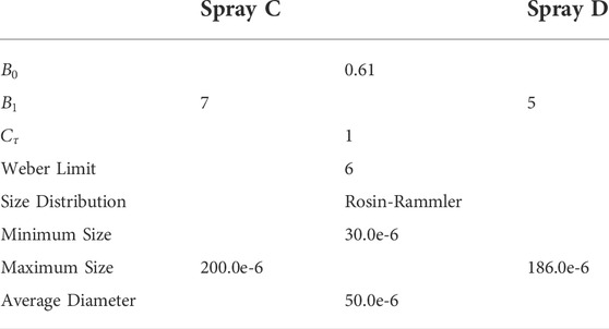
TABLE 1. Breakup model specifications for Spray C and Spray D.
Case description
As stated in the Introduction, the ECN cases examined in this study are Spray C and Spray D. The inert-condition cases are allowed to develop for 3 ms, whereas the reacting-condition cases develop for 5 ms. Injection starts at the beginning of the simulation. In all cases, a single-orifice injection of n-dodecane at 150 MPa is employed, and the ambient conditions are identical (temperature, density, and species concentrations). The details are summarized in Table 2. The models and simulations are implemented and run in OpenFOAM software (OpenFOAM v7, 2020). The geometry, position of the injector (Figure 1), and all computational parameters are identical for both sprays modelled using both RANS and LES frameworks. The domain is represented by a cylinder with the injector on top, a square central refinement (for improved capturing of the spray and spatial distribution of the species), a total length of 140 mm, and a diameter of 47.612 mm. The extent of the domain is chosen such that it does not influence the flow. All boundaries apart from the ceiling are considered open (for details please refer to Table 3 where the most important boundary parameters are summarized).
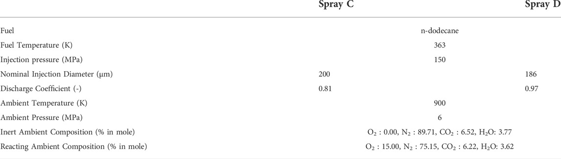
TABLE 2. Specifications for ECN Spray C and Spray D (ECN, 2022).
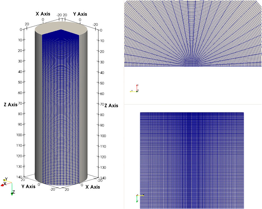
FIGURE 1. Cylinder dimensions and central refinement.
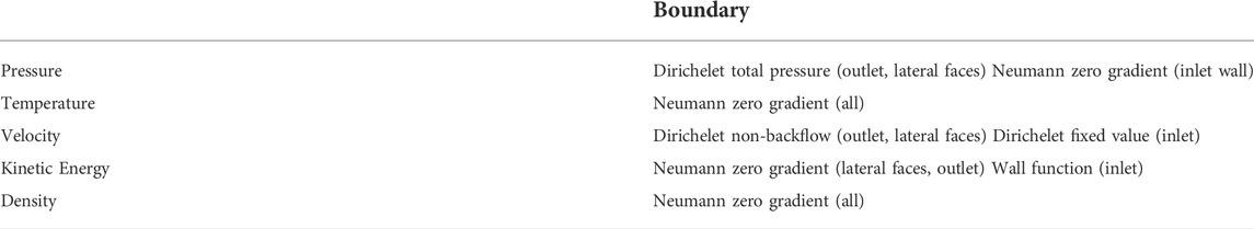
TABLE 3. Most important boundary settings.
Meshes are created using the blockMesh utility in OpenFOAM, which allows relatively straightforward creation of a structured mesh with simple geometries. All meshes, for both benchmarks and turbulence models, are created from a base cell size which represents the cell size on top of the central refinement squared region along the spray axis. This base cell is subsequently stretched towards the bottom and lateral walls of the cylinder, following a cell-to-cell expansion ratio. Different values for the base mesh size are used to investigate the convergence of the mesh.
Results and discussion
Model validation RANS
The major difference between the RANS and LES setups is the mesh; the RANS turbulence model allows the use of coarser meshes; the primary advantage of RANS simulations compared with LES models. Base cell sizes of 150 μm, 175 μm, 200 μm, 225 μm, 250 μm, and 300 μm are used for validation. The spray behavior for inert cases is analyzed in terms of the liquid length and the spray tip penetration. To assess the performances of both approaches, the inert cases are initially studied. The results from this will allow the mesh requirements to be set. Both the liquid length, defined as the distance from the nozzle containing 95% of the injected mass, and the spray tip penetration, defined as the farthest point from the injection point exhibiting a threshold value for fuel vapor mass concentration of 0.001 (Egüz et al., 2012), are compared with experimental results.
Since the principal goal of this work is a direct comparison of the RANS and LES models keeping the numerical set-up as similar as possible, a compromise, in terms of the performance achieved by all cases, was made in the choice of breakup model constants and discretization schemes. Thus, the analyzed vapor penetrations and liquid lengths perform relatively poorly in the single case, and the liquid length is unstable. The Appendix contains the vapor penetrations and liquid lengths for Spray C and Spray D in the RANS framework, providing an overview of any fine tuning required for each specific case [for the LES framework, refer to Bao et al. (2022)].
Spray C, inert
Figure 2 shows the results for Spray C.
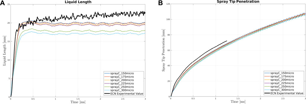
FIGURE 2. Liquid Length (A) and Spray Tip Penetration (B) for Spray C at various mesh dimensions.
As seen in Figure 2A the agreement with experimental data appears to be suitable for all mesh sizes, except for those with the largest base mesh sizes (250 μm and 300 μm), which exhibit considerably lower values. This relationship between the liquid length and the cell dimension is expected and is well-known. Indeed, the finer the mesh, the slower the evaporation since a smaller cell leads to faster saturation (Karr̈Holm and Nordin, 2005), hence the longer liquid penetration for smaller cells. Typical liquid length behavior: an initial transient period followed by stabilization close to an average value (Siebers, 1998), is well reproduced. A plateau is reached after the two largest cell sizes, which are well below the experimental value. Further refinement of the base mesh size does not result in an improved liquid length compared with the experimental curve.
Figure 2B presents the spray tip penetration. Importantly, a suitable correspondence with the experimental data, close to the time when ignition generally occurs (0.58 ms for Spray C at 900 K) is observed. The agreement is not perfect since a distinct difference in the injection is observed at the initial stage. This issue seems to be correlated to the time step independency, which may be remedied by using a limiter on the turbulence length scale equal to the nozzle diameter, as suggested by Karr̈Holm and Nordin (2005); however this is a matter for future studies. Furthermore, it should be noted that at the present time, an accurate trace of the spray tip penetration up to 3 ms is not available. Although the experimental value could be extrapolated to 3 ms, the result was not realistic; hence we avoided it in this study. However, all meshes appear to agree well with the experimental data, except the two coarsest which appear to display slower vapor penetrations; a direct consequence of the presence of additional liquid in the larger cell sizes. Since we must consider a good compromise in terms of computational effort hereafter, a mesh size of 225 μm (counting 747,643 cells) is chosen as the base mesh size for Spray C.
Spray D, inert
All above considerations for Spray C are also valid for Spray D. The geometry is identical, with the only differences being the nozzle diameter, the rate of injection, and the total mass injected. All other parameters are kept constant, and the six base sizes chosen for Spray C are also analyzed for Spray D. Figure 3 shows the liquid lengths and spray tip penetrations for Spray D.
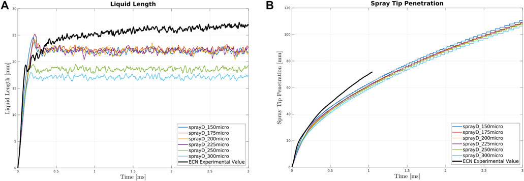
FIGURE 3. Liquid Length (A) and Spray Tip Penetration (B) for Spray D at various mesh dimensions.
A deviation from the experimental data is observed for the liquid length. After the first transient period, a clear peak in the instantaneous liquid length occurs; this is not observed in either Spray C or in the experimental data. This may be related to the numerical issue mentioned previously for the Spray C tip penetration, and requires further investigation. The mesh size trend highlighted in the Spray C section is also observed here; after an initial improvement in the performance upon refining the mesh, no further improvement in the average liquid length value occurs. Again, the coarsest meshes exhibit inferior performances.
The experimental ignition delay for Spray D is 0.59 ms and the difference between the experimental data and the model at this time is slightly larger than that observed for Spray C. Importantly, Spray D penetrates more rapidly than Spray C, in agreement with previous experimental observations (Pastor et al., 2018; Westlye et al., 2016). Similar to Spray C, the experimental data for Spray D do not reach 3 ms; extrapolation resulted in unrealistic results which were not used.
Since the two sprays do not require different base mesh sizes, a mesh size of 225 μm will be used for both hereafter, allowing coherent comparison of the two benchmarks.
Model validation LES
The above approach was also used here; however, a smaller number of base mesh sizes was analyzed. There are two reasons for this: firstly, the computational effort required here is higher since the meshes are approximately twice as large as the most refined mesh in the RANS analysis; secondly, one of the meshes analyzed here (named 125 µm lessRef) was used in a previous study (Bao et al., 2022). The validation in this previous study uses the same LES approach as in this work and the results in terms of spray tip penetration, liquid length, and distribution of mixture fraction and its variance are respectable. Therefore, this analysis begins from the reference dimension and adds one larger and one smaller base size in order to explore the mesh dependence.
Spray C, inert
In Figure 4, the liquid lengths and spray tip penetrations of Spray C are shown for the inert case, using four different base cell sizes: 100 μm, 125 μm, 125 µm (which is less refined in the radial direction), and 150 µm.
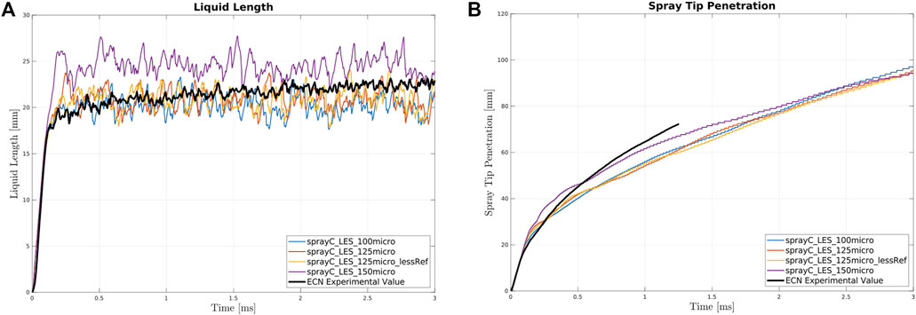
FIGURE 4. Liquid Length (A) and Spray Tip Penetration (B) for Spray C at various mesh dimensions.
The liquid length graph shows small differences in the results where the trace stabilizes after the first transient element. In the RANS simulations, the difference in the various mesh sizes was significantly larger, with the two coarsest meshes performing noticeably worse than other sizes. Here, the only major deviation is observed for the coarsest mesh (150 µm), which yields a higher average liquid length value. This does not follow the relationship between the mesh size and the liquid length previously observed (Karr̈Holm and Nordin, 2005), and verified in the RANS validation section. The spray tip penetration agrees well with the relationship described above; the coarsest mesh presents the fastest evaporation. However, this is not an anomaly since more realizations are required to achieve improved statistical convergence. Another notable difference compared with the inert validation presented for the RANS model, is the considerably larger fluctuations in the average liquid length values. This is due to the nature of the two turbulence models: the RANS model provides an average of the fluctuations, whereas the LES model solves them (up to a defined size).
The first transient phase, in contrast to the RANS results, is perfectly reproduced by all meshes until approximately 0.15 ms, where differences begin to appear. Apart from the coarsest mesh, other meshes appear to behave similarly. Interestingly, although the first transient is reproduced, the maximum value reached at 3 ms is lower, even for the coarsest mesh which began with a significantly steeper slope. The turbulent fluctuations observed in the LES model significantly affect the spray, shortening the maximum length reached.
In conclusion, as far as Spray C simulations are concerned, the mesh size named 125 µm_lessRef (a larger mesh size in the radial dimension of the cylinder compared with the full 125 µm mesh) is chosen for further simulations. The mesh convergence for both the liquid length and the tip penetration appears to be achieved for the three most refined meshes. Therefore, in order to limit the computational effort required, and to possess a well-tested benchmark (Bao et al., 2022), the coarsest mesh (counting 2,755,584 cells) of the three most refined is used in the combustion analysis.
Spray D, inert
Figure 5 shows the inert results for Spray D; the same Spray C mesh base sizes were also analyzed here.
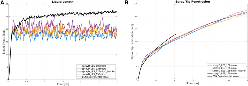
FIGURE 5. Liquid Length (A) and Spray Tip Penetration (B) for Spray D at various mesh dimensions.
The observations made in the previous section can also be made here. Figure 5A clearly shows that the coarsest mesh performs worse than the others (150 µm); however, not to the extent observed for Spray C. Notably, all meshes perform worse in terms of the liquid length compared with Spray C. This can be explained by firstly considering the behavior previously highlighted in the RANS analysis of Spray D, which exhibits a peak after the first transient injection period and subsequently levels out to the average liquid length. The value obtained is lower than the experimental value. Secondly, the average experimental value is larger than that of Spray C. Consequently, the model clearly performs worse for Spray D than for Spray C.
For the spray tip penetration, the results are coherent with experimental results until approximately 1 ms. Notably, the model correctly reproduces the behavior previously observed for the RANS simulations; Spray D penetrates faster than Spray C. Moreover, the initial component of the penetration is perfectly reproduced; however, the initial change in slope provided by the simulation (∼0.12 ms) occurs after the experimental data. This is unlike Spray C, where the considerably steeper change in slope occurs at the same time as the experimental data. The net result is that the penetration around the IDT (∼0.5 ms) is significantly closer to the experimental value compared with Spray C. The Spray D penetration for all meshes is similar: the curve for the coarsest mesh is closer to the others than what is observed for Spray C.
Since the mesh performances appear to be decent in all cases, and since the use of one mesh for both benchmarks would lower the associated computational power, the same sized mesh as that chosen for Spray C is used for the remainder of the study.
Reacting cases analysis
In this section, the most important combustion performance indicators are presented. In particular, the ignition delay time (IDT), lift-off length (LOL), and species distribution along the flame are the key factors considered. These are analyzed for Spray C and Spray D and compared across the RANS and LES turbulence models.
Before proceeding with the analysis, a number of points should be considered: for the LES model, only one realization of the reacting case has been conducted. It has been shown previously (Bao et al., 2022) that more than one realization in the LES framework is required to obtain statistical convergence of certain quantities (
Moreover, the transient development of the flame in both turbulence models as well as in all reacting cases is evaluated using so-called
where the intensity,
It should be noted that
Spray C, reacting
Figure 6 shows the
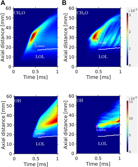
FIGURE 6.
LES and RANS models present similarly-shaped
The highest
Figure 7 presents a temporal evolution of Spray C. The visualization is divided into three groups representing three periods of time: the period prior to ignition (0.2–0.5 ms), the period directly after ignition (0.7–1.5 ms), and the quasi-steady period (2–3 ms). For each period three rows are provided; the second row represents the
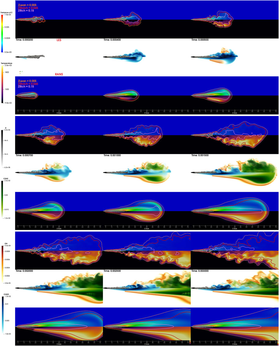
FIGURE 7. Spray C flame evolution from 0.2 ms to 3 ms. The image is divided into three parts: from 0.2 to 0.5 ms, from 0.7 to 1.5 ms, and from 2 to 3 ms. Each part is further divided into three: the central image represents OH, CH2O, and C2H2 for the LES (upper) and RANS (lower) frameworks. The surrounding images are the temperature distribution, the variance of the mixture fraction, and three contours of the mixture fraction (lean, stoichiometric, and rich).
Clearly, as observed in the
Spray D, reacting
Figure 8 shows the
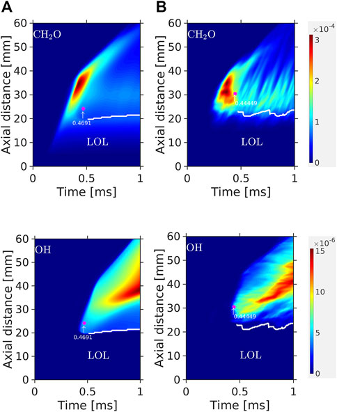
FIGURE 8.
The observations here are similar to those made for Spray C. The low-temperature zone indicated by the
For clarity, Table 4 lists the values of the primary combustion parameters.
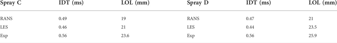
TABLE 4. Most important combustion parameters for Spray C (left) and Spray D (right) from simulations and experiments.
Figure 9 shows the flame evolution, similar to Figure 7. The observed behavior is comparable to above;
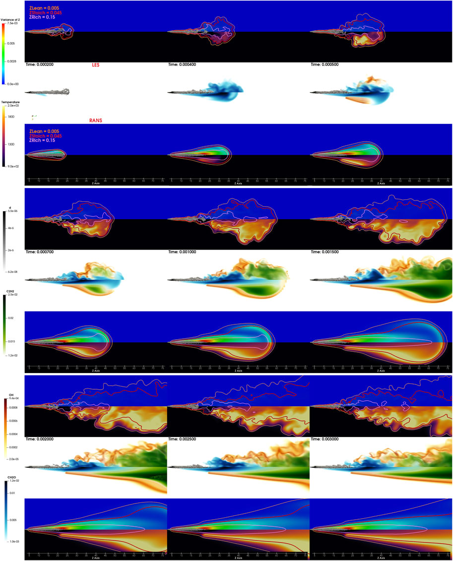
FIGURE 9. Spray D flame evolution from 0.2 ms to 3 ms. The image is divided into three parts: from 0.2 to 0.5 ms, from 0.7 to 1.5 ms, and from 2 to 3 ms. Each part is further divided into three: the central image represents OH, CH2O, and C2H2 for the LES (upper) and RANS (lower) frameworks. The surrounding images are the temperature distribution, the variance of the mixture fraction, and three contours of the mixture fraction (lean, stoichiometric, and rich).
Conclusion
In this study, the Spray C and Spray D ECN benchmarks were analyzed using the same solver (OpenFOAM) and the same combustion model (FGM). The performances of the RANS and LES turbulence models were compared, using the FGM combustion model with four-dimensional tabulation. The agreement with experiments, in terms of the liquid length and the spray tip penetration, are respectable for both turbulence models. For the reacting sprays, both the RANS and LES simulations reproduce the experimental observation that Spray C exhibits a shorter lift-off length, while the ignition delay for Spray D is shorter. In general, the ignition delays predicted by both turbulence models are shorter than the experimental values for both sprays. The RANS model predictions for the IDT are slightly longer than their LES counterparts, with ignition occurring closer to the nozzle outlet. The local characteristics of the markers for low-temperature chemistry (
In conclusion, both the RANS and LES models, coupled with the FGM combustion model, provide an excellent insight into the characteristics of the two ECN sprays, since the two methods provide similar results to experiments. The primary benefit of the LES model is the reproduction of the instantaneous flame shape and the species distribution, a natural consequence of a more precise turbulence chemistry interaction. Nevertheless, the RANS model remains a good choice in terms of efficiency since the required computational effort is lower and the primary parameter reproduction is close to that achieved by the LES model. This is important because it indicates the reliability of this turbulence model, which will be particularly useful for future studies where the computational domains will be significantly larger than that analyzed here.
Data availability statement
The raw data supporting the conclusion of this article will be made available by the authors, without undue reservation.
Author contributions
Corresponding author (ADM) is the first author, who wrote the article, performed simulations and post processing, coding. Second author (HB) helped in interpretation of results, coding and writing style. Third author (BS) is first author supervisor and helped in interpretation of results and writing style.
Funding

This project has received funding from the European Union’s Horizon 2020 research and innovation program under grant agreement No 883753.
Conflict of interest
The authors declare that the research was conducted in the absence of any commercial or financial relationships that could be construed as a potential conflict of interest.
Publisher’s note
All claims expressed in this article are solely those of the authors and do not necessarily represent those of their affiliated organizations, or those of the publisher, the editors and the reviewers. Any product that may be evaluated in this article, or claim that may be made by its manufacturer, is not guaranteed or endorsed by the publisher.
References
Bao, H., Maes, N., Akargun, H. Y., and Somers, B. (2022). Large Eddy Simulation of cavitation effects on reacting spray flames using FGM and a new dispersion model with multiple realizations. Combust. Flame 236, 111764. doi:10.1016/j.combustflame.2021.111764
Bao, H., Kalbhor, A., Maes, N., Somers, B., and Van Oijen, J. (2022). Investigation of soot formation in n -dodecane spray flames using LES and a discrete sectional method. Proc. Combust. Inst. S1540748922001183. doi:10.1016/j.proci.2022.07.089
Bharadwaj, N., Rutland, C. J., and Chang, S. (2009). Large eddy simulation modelling of spray-induced turbulence effects. Int. J. Engine Res. 10, 97–119. doi:10.1243/14680874JER02309
Bhattacharjee, S., and Haworth, D. C. (2013). Simulations of transient n-heptane and n-dodecane spray flames under engine-relevant conditions using a transported PDF method. Combust. Flame 160, 2083–2102. doi:10.1016/j.combustflame.2013.05.003
Bilger, R. W., Stårner, S. H., and Kee, R. J. (1990). On reduced mechanisms for methane-air combustion in nonpremixed flames. Combust. Flame 80, 135–149. doi:10.1016/0010-2180(90)90122-8
Dahms, R. N., Paczko, G. A., Skeen, S. A., and Pickett, L. M. (2017). Understanding the ignition mechanism of high-pressure spray flames. Proc. Combust. Inst. 36, 2615–2623. doi:10.1016/j.proci.2016.08.023
Desantes, J. M., Garcia-Oliver, J. M., Novella, R., and Pachano, L. (2020). A numerical study of the effect of nozzle diameter on diesel combustion ignition and flame stabilization. Int. J. Engine Res. 21, 101–121. doi:10.1177/1468087419864203
ECN, Engine combustion network, 2022, (Available at: https://ecn.sandia.gov/).
Egüz, U., Ayyapureddi, S., Bekdemir, C., Somers, B., and de Goey, P., 2012. Modeling fuel spray auto-ignition using the FGM approach: Effect of tabulation method. SAE 2012 World Congress & Exhibition, Detroit, MI, April 24, 2012, pp. 2012-01–0157. doi:10.4271/2012-01-0157
García-Oliver, J. M., Malbec, L.-M., Toda, H. B., and Bruneaux, G. (2017). A study on the interaction between local flow and flame structure for mixing-controlled Diesel sprays. Combust. Flame 179, 157–171. doi:10.1016/j.combustflame.2017.01.023
García-Oliver, J. M., Novella, R., Pastor, J. M., and Pachano, L. (2020). Computational study of ECN Spray A and Spray D combustion at different ambient temperature conditions. Transp. Eng. 2, 100027. doi:10.1016/j.treng.2020.100027
Ge, H.-W., and Gutheil, E. (2006). Probability density function (PDF) simulation of turbulent spray flows. At. Spr. 16, 531–542. doi:10.1615/AtomizSpr.v16.i5.40
Higgins, B., and Siebers, D., Measurement of the flame lift-off location on dl diesel sprays using O H chemiluminescence, SAE Technical paper, 17. 2001.
Karr̈Holm, F. P., and Nordin, N. (2005). “Numerical investigation of mesh/turbulence/spray interaction for diesel applications,” in Paper i proceeding, 2005, Rio De Janiero, Brazil, May 11, 2005, 2005-01–2115. doi:10.4271/2005-01-2115
Liu, K., and Haworth, D. C. (2011). Development and assessment of POD for analysis of turbulent flow in piston engines. SAE Tech. Pap., 2011-01–0830. doi:10.4271/2011-01-0830
Maes, N., Meijer, M., Dam, N., Somers, B., Baya Toda, H., Bruneaux, G., et al. (2016). Characterization of Spray A flame structure for parametric variations in ECN constant-volume vessels using chemiluminescence and laser-induced fluorescence. Combust. Flame 174, 138–151. doi:10.1016/j.combustflame.2016.09.005
Maes, N., Skeen, S. A., Bardi, M., Fitzgerald, R. P., Malbec, L.-M., Bruneaux, G., et al. (2020). Spray penetration, combustion, and soot formation characteristics of the ECN Spray C and Spray D injectors in multiple combustion facilities. Appl. Therm. Eng. 172, 115136. doi:10.1016/j.applthermaleng.2020.115136
Ong, J. C., Pang, K. M., Bai, X.-S., Jangi, M., and Walther, J. H. (2021). Large-eddy simulation of n-dodecane spray flame: Effects of nozzle diameters on autoignition at varying ambient temperatures. Proc. Combust. Inst. 38, 3427–3434. doi:10.1016/j.proci.2020.08.018
OpenFOAM v7 (2020). OpenFOAM v7. Available at: https://cpp.openfoam.org/v7/.
Pastor, J. V., Garcia-Oliver, J. M., Garcia, A., and Morales López, A. (2018). “An experimental investigation on spray mixing and combustion characteristics for spray C/D nozzles in a constant pressure vessel,” in Proceedings of the International Powertrains, Fuels & Lubricants Meeting, Heidelberg, Germany, September 17, 2018, 2018-01–1783. doi:10.4271/2018-01-1783
Payri, F., García-Oliver, J. M., Novella, R., and Pérez-Sánchez, E. J. (2019). Influence of the n-dodecane chemical mechanism on the CFD modelling of the diesel-like ECN Spray A flame structure at different ambient conditions. Combust. Flame 208, 198–218. doi:10.1016/j.combustflame.2019.06.032
Pei, Y., Hawkes, E. R., Bolla, M., Kook, S., Goldin, G. M., Yang, Y., et al. (2016). An analysis of the structure of an n-dodecane spray flame using TPDF modelling. Combust. Flame 168, 420–435. doi:10.1016/j.combustflame.2015.11.034
Pei, Y., Som, S., Pomraning, E., Senecal, P. K., Skeen, S. A., Manin, J., et al. (2015). Large eddy simulation of a reacting spray flame with multiple realizations under compression ignition engine conditions. Combust. Flame 162, 4442–4455. doi:10.1016/j.combustflame.2015.08.010
Peters, N. (1984). Laminar diffusion flamelet models in non-premixed turbulent combustion. Prog. Energy Combust. Sci. 10, 319–339. doi:10.1016/0360-1285(84)90114-X
Pickett, L. M., Manin, J., Genzale, C. L., Siebers, D. L., Musculus, M. P. B., and Idicheria, C. A. (2011). Relationship between diesel fuel spray vapor penetration/dispersion and local fuel mixture fraction. SAE Int. J. Engines 4, 764–799. doi:10.4271/2011-01-0686
Pickett, L. M., Siebers, D. L., and Idicheria, C. A. (2005). “Relationship between ignition processes and the lift-off length of diesel fuel jets,” in Proceedings of the Powertrain & Fluid Systems Conference & Exhibition, San Antonio, TX, October 24, 2005, 2005-01–3843. doi:10.4271/2005-01-3843
Pierce, C. D., and Moin, P. (1998). A dynamic model for subgrid-scale variance and dissipation rate of a conserved scalar. Phys. Fluids 10, 3041–3044. doi:10.1063/1.869832
Reitz, R. D. (1987). “Modeling atomization processes in high pressure vaporizing sprays,” in At. Sprays Technol 3, 309–337.
Salehi, M. M., and Bushe, W. K. (2010). Presumed PDF modeling for RANS simulation of turbulent premixed flames. Combust. Theory Model. 14, 381–403. doi:10.1080/13647830.2010.489957
Siebers, D. L., 1998. Liquid-phase fuel penetration in diesel sprays. Technical paper, p. 980809. doi:10.4271/980809
Som, S., Longman, D. E., Lu, Z., Plomer, M., Lu, T., Senecal, P. K., et al. (2011). “Simulating flame lift-off characteristics of diesel and biodiesel fuels using detailed chemical-kinetic mechanisms and LES turbulence model,” in Proceedings of the Internal Combustion Engine Division Fall Technical Conference (ICEF), Morgantown, WV, October 2, 2011, 12.
Somers LMT (Bart) (1994). The simulation of flat flames with detailed and reduced chemical models. Eindhoven, Netherlands: Doctor of Philosophy, Mechanical Engineering. doi:10.6100/IR420430
Tsang, C.-W., Kuo, C.-W., Trujillo, M., and Rutland, C. (2019). Evaluation and validation of large-eddy simulation sub-grid spray dispersion models using high-fidelity volume-of-fluid simulation data and engine combustion network experimental data. Int. J. Engine Res. 20, 583–605. doi:10.1177/1468087418772219
Oijen van, J. A. (2002). Flamelet-generated manifolds : Development and application to premixed laminar flames. Eindhoven: Doctor of Philosophy, Mechanical Engineering. doi:10.6100/IR557848
Wehrfritz, A., Kaario, O., Vuorinen, V., and Somers, B. (2016). Large eddy simulation of n-dodecane spray flames using flamelet generated manifolds. Combust. Flame 167, 113–131. doi:10.1016/j.combustflame.2016.02.019
Westlye, F. R., Battistoni, M., Skeen, S. A., Manin, J., Pickett, L. M., and Ivarsson, A. (2016). “Penetration and combustion characterization of cavitating and non-cavitating fuel injectors under diesel engine conditions,” in Proceedins of the SAE 2016 World Congress and Exhibition, Detroit, MI, April 12, 2016, 2016-01–0860. doi:10.4271/2016-01-0860
Yao, T., Pei, Y., Zhong, B.-J., Som, S., Lu, T., and Luo, K. H. (2017). A compact skeletal mechanism for n-dodecane with optimized semi-global low-temperature chemistry for diesel engine simulations. Fuel 191, 339–349. doi:10.1016/j.fuel.2016.11.083
Zhang, Y., Wang, H., Both, A., Ma, L., and Yao, M. (2019). Effects of turbulence-chemistry interactions on auto-ignition and flame structure for n-dodecane spray combustion. Combust. Theory Model. 23, 907–934. doi:10.1080/13647830.2019.1600722
Appendix
Figure A1 and Figure A2 reported vapor penetration and liquid length of Spray C and Spray D in RANS with fine tuning of the break-up model constants for the specific benchmark and turbulence model. The comparison is between the results obtained using the constants adopted in this work for compromise and the results obtained using constants obtained fine tuning each case alone.
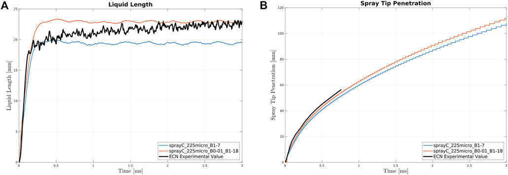
FIGURE A1. Liquid Length (A) and Spray Tip Penetration (B) for Spray C at varying break-up constants: in blue the one used in this work, in orange the optimized one.
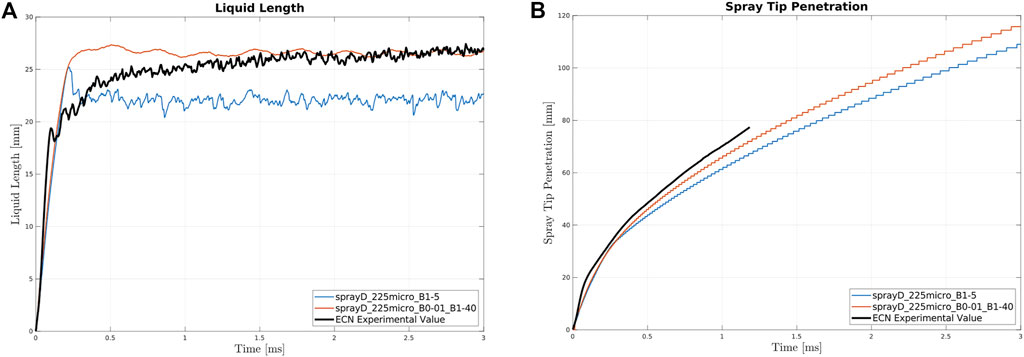
FIGURE A2. Liquid Length (A) and Spray Tip Penetration (B) for Spray D at varying break-up constants: in blue the one used in this work, in orange the optimized one.
Keywords: spray modeling, ECN, spray C, spray D, FGM, RANS, LES
Citation: Di Matteo A, Bao H and Somers B (2022) Modeling Spray C and Spray D with FGM within the framework of RANS and LES. Front. Mech. Eng 8:1013138. doi: 10.3389/fmech.2022.1013138
Received: 06 August 2022; Accepted: 03 October 2022;
Published: 10 November 2022.
Edited by:
Tiemin Xuan, Jiangsu University, ChinaReviewed by:
Hu Wang, Tianjin University, ChinaYanzhi Zhang, Jiangsu University, China
Zongyu Yue, Tianjin University, China
Copyright © 2022 Di Matteo, Bao and Somers. This is an open-access article distributed under the terms of the Creative Commons Attribution License (CC BY). The use, distribution or reproduction in other forums is permitted, provided the original author(s) and the copyright owner(s) are credited and that the original publication in this journal is cited, in accordance with accepted academic practice. No use, distribution or reproduction is permitted which does not comply with these terms.
*Correspondence: Andrea Di Matteo, YS5kaS5tYXR0ZW9AdHVlLm5s