A novel approach to estimate power demand of auxiliary engine loads of light duty vehicles

1 Introduction

In order to align with sustainable development targets, regulations and goals for fuel economy and emissions have been imposed at both the national and international level. When developing policies related to sustainable road transportation and related energy consumption, it is important to identify the factors contributing to increased energy consumption and to develop a baseline model using both theoretical and empirical approaches. The major sources of power demand in a light duty vehicle (LDV) are the energy needed to overcome the aerodynamic drag resistance, rolling resistance, grade resistance, and inertial resistance. Auxiliary equipment is also assumed to be a major drain on power and its impact was measured and quantified in this study. The research scope encompassed the main auxiliary devices, the air-conditioning unit, the alternator, water pump, and power-steering pump. In the next section, we review the literature on this subject, discuss the findings, and identify the gaps in the previous work.

Several previous studies have been carried out by researchers to evaluate the impact of auxiliary engine loads on the overall power demand and fuel consumption of a given vehicle. The report by Welstand et al. (2003) revealed that belt-driven auxiliary units had a close, proportional relationship with engine speed, with higher power demand at higher engine speeds. The study found that during normal engine idling (800–1000 RPM), the auxiliary power demand was 1.75 kW with the air-conditioning (A/C) unit turned off and 3.25 kW with the A/C turned on. At a higher engine speed of around 3000 RPM, the auxiliary power demand increased to 9–9.5 kW with the A/C on. Also, the A/C system required a higher driving torque than any other auxiliary equipment. A common characteristic of engine belt-driven auxiliary units is that their input power for operation is proportional to the engine speed, while their output power may not be related to engine speed. The study conducted by Nadamoto and Kubota revealed that the compressor was the most significant component affecting the power demand because it was responsible for a 77–89% increase in energy consumption (Nadamoto and Kubota, 1999). The impact on energy demand of the subordinate components has been determined and is 6–12% from the blower, 4–10% from the cooling fan, and 0.7–2% from the clutch (Nadamoto and Kubota, 1999). The A/C system plays a crucial role when it comes to electric vehicles (EVs), including both hybrid electric vehicles (HEVs) and battery electric vehicles (BEVs). EVs have insufficient waste heat to warm up the cabin and the climate control system has a substantial effect on the energy consumption efficiency and operating range. The mobile climate control systems based on the magnetocaloric and thermoelectric effects could be utilized to optimize the range efficiency (Zhaogang, 2014). The vapor compression refrigeration-dedicated, combination heater-A/C systems, reversible vapor compression heat pump A/C systems, and non-vapor compression A/C systems have been critically appraised by Zhang et al. (2018) as the latest developments in air-conditioning and heat pump systems for EVs.

The vehicle’s water pump may be mechanical or electric. The major drawback of a mechanical pump is that it pumps in proportion to engine speed and not according to the heat rejection requirements (Tasuni et al., 2016). Hence, it is necessary to evaluate the operating characteristics of the water pump and its impact on fuel consumption. In general, 1–2 kW of power is transferred from the crankshaft to the water pump (Patel et al., 2013). The efficiency of a water pump is quite low due to its losses. According to the published data, the mechanical efficiency of a water pump typically lies between 37.5% and 55.0% within an RPM range of 2,000–5,000, respectively (Wang et al., 2015a). The lack of efficiency in the water pump operation can be attributed to three main causes: mechanical, hydraulic, and volumetric losses (Tasuni et al., 2016). The mechanical losses result from friction associated with the dynamic parts of the pump, hydraulic losses occur as internal losses in the impeller, while volumetric losses are due to the leakage of liquid from the discharge side to the suction side of the centrifugal pump (Tasuni et al., 2016).

There has been an increasing demand for electric power since automotive technological advancements have replaced many of the mechanical devices with electrical and electronic devices. Two major evolutions in automobile electrical systems can be stated: the change from 6V to 12V systems and the switch from DC generators to AC alternators (Cho et al., 2008). The AC alternator can be considered as the most important piece of equipment in the electrical system. The electrical power of a vehicle is generated as a direct result of the engine consuming fuel to drive the alternator (Bradfield, 2008). With a nominal efficiency level of 40% in the engine, 98% in the belt-train and 55% in the alternator, the electrical generation system has an overall efficiency of around 21% (Bradfield, 2008). With regard to the losses in the alternator, they can be stratified into three types: electrical, magnetic, and mechanical (Bradfield, 2008). The consensus in the literature, states that in general, the output power losses increase with increasing engine speed. Consequently, the increase in alternator losses can be said to be proportional to the increase in operating fuel consumption.

Nowadays, most of the previously belt-driven engine auxiliaries are driven by electricity. For example, the water/coolant pump and the power steering pump are more often electrically powered. Furthermore, with the increasing utilization of electric vehicles (EVs), including HEVs and BEVs, the necessity for electrically powering auxiliaries has increased. Estimating the power demand of the auxiliary loads is thus of greater importance than ever, since it directly affects an EV’s range and could enhance the range anxiety of users (Roskilly et al., 2015) (Weldon et al., 2016). The approach proposed by this study could eventually result in the development of a range prediction algorithm for EVs. Accurate range prediction is the key to minimizing range anxiety and helping drivers make the best use of their available energy (Wu et al., 2015) (Cuma and Koroglu, 2015). Thus, an accurate theoretical model is required to determine the major auxiliary load contributors, which is a major focus of this study.

In most of the previously published work, the auxiliary load determinations were performed using experimental evaluations, whereas in the proposed study, each sub-auxiliary system was analytically appraised using the governing equations, which can be considered a new contribution of this study. Against the empirical approach adopted in the literature, this study delves into a theoretical approach, especially pertaining to the determination of AC load. In the next sections, the power demands of the AC system, the alternator, the mechanical water pump, and the power-steering pump are characterized and analyzed.

2 Modeling and estimating the power demand of an automotive air conditioner

The AC unit is an auxiliary device designed to ensure the comfort of the passengers by regulating the temperature and the relative humidity (RH) within the cabin. The AC system consists of the compressor, the belt, the blower, the cooling fan, the condenser, the receiver/drier, inline filter kit, expansion valve, hose assembly, and evaporator core. In this section, the AC load is theoretically modeled, and the total AC load is determined by the summation of the individual heat load contributors.

$Q_{Total}=Q_{Met}+Q_{Rad}+Q_{Amb}+Q_{Exh}+Q_{Eng}+Q_{Ven.}(1)$

Eq. 1 gives the summation of the major contributors to automotive AC load. Each of these load types will be discussed under the following sections and the total AC load, ($Q_{Total}$) will be modeled. In Eq. 1, $Q_{Total}$ denotes the total AC load, $Q_{Met}$ is the metabolic load, $Q_{Rad}$ is the radiation load, $Q_{Amb}$ is the ambient load, $Q_{Exh}$ is the exhaust load, $Q_{Eng}$ is the engine load, and $Q_{Ven}$ is the ventilation load.

2.1 Modeling of metabolic load

Heat is dissipated from the human body as a result of metabolism, and this specific type of heat load also contributes to the total heat load of the AC. The metabolic load has two main components: the sensible heat load and the latent heat load. The sensible heat load refers to the heat given off from the human body by convection and radiation, whereas the latent heat load refers to the heat dissipated through evaporation.

$Q_{Met}=Q_{Sensible}+Q_{Latent},(2)$

$Q_{Sensible}$ and $Q_{Latent}$ can be determined using the formulas stated in Eqs 3, 4.

$Q_{Sensible}={\displaystyle \sum }_{Passengers}{M_{Sensible}A}_{Du,}(3)$

$Q_{Latent}={\displaystyle \sum }_{Passengers}{M_{Latent}A}_{Du.}(4)$

In Eqs 6, 7, $M_{Sensible}$ and $M_{Latent}$ are the sensible metabolic heat production rate and the latent metabolic heat production rate, respectively, obtained from the tabulated values in ISO 8986 (ISO, 1989). When determining the metabolic load, an estimation of the body surface area $A_{Du}$ as a function of height and weight is calculated using Eq. 5.

$A_{Du}=0.21W^{0.425}{H}^{0.725}.(5)$

In Eq. 9, $W$ and $H$ denote the weight and height of a human. Since the study focuses mainly on local context, an average height and weight for a Sri Lankan person were determined and used as reference. The average height of a Sri Lankan, regardless of the gender is around 162.0 cm, and the average weight (in 2015) is around 61.4 kg (WHO, 2015), (Martinez et al., 2020). Eqs 3, 4 require the number of passengers to be estimated, and in a road vehicle travelling in Sri Lanka, the average number of occupants is two: one driver and one passenger. The average metabolic load contributed by the vehicle’s occupants performing different activities is depicted in Table 1 (Havenith et al., 2002).

TABLE 1

TABLE 1. Metabolic load calculation of a passenger car. Data taken from (Martinez et al., 2020).

The total sensible heat production rate of two passengers within a vehicle is determined by Eq. 6, whereas the total latent heat production rate is determined as in Eq. 7. When determining the metabolic rates of the occupants, the driver’s metabolic rate is considered with respect to moderate arm work since the driver is actively engaged in the task of driving, whereas the passenger is assumed to be just sitting.

$M_{Sensible}=105W{m}^{-2}(6)$

$M_{Latent}=155W{m}^{-2}(7)$

Hence, total metabolic load can be determined using Eqs 8, 9.

$Q_{Sensible}={\displaystyle \sum }_{passengers}^2{M}_{Sensible}{\overline{A}}_{DU},(8)$

$Q_{Latent}={\displaystyle \sum }_{passengers}^2{M}_{Latent}{\overline{A}}_{DU}(9)$

In Eqs 8, 9, ${\overline{A}}_{DU}$ denotes mean human body surface area using the Du Bois method (Fayazbakhsh and Bahrami, 2013). The estimated body area of an average passenger is determined in the following calculation performed, and the result is ${\overline{A}}_{DU}$ = 1.72 m², as stated in Eq. 10.

${\overline{A}}_{DU}=0.21\left({61.4}^{0.425}\right)\left({1.62}^{0.725}\right)$

${\overline{A}}_{DU}=0.21\left(5.75\right)\left(1.42\right),$

${\overline{A}}_{DU}=1.72{\mathrm{m}}^2(10)$

Then, using the determined values for $M_{Sensible}$, $M_{Latent}$, and ${\overline{A}}_{DU}$ substituted in Eqs 8, 9, the sensible heat load $Q_{Sensible}$ and the latent heat load $Q_{Latent}$ of an AC are determined as follows:

$Q_{Sensible}=105\left(1.72\right)$

${\begin{array}{c}\\ Q\end{array}}_{Sensible}=\mathbf{180.60}\mathit{W}(11)$

$Q_{Latent}=155\left(1.72\right)$

$Q_{Latent}=\mathbf{266.66}\mathit{W}(12)$

Thus, the mean metabolic load of a car with two passengers in a local context can be modeled as portrayed in this section. The estimated mean metabolic heat load for an average car plus two occupants is calculated to be 447.26 W.

Figure 1 depicts a three-dimensional distribution of the metabolic heat load on par with the variation in body surface area using the Du Bois method for a two-occupant car cabin (a driver with medium arm work and one passenger at rest). The colored bar represents the intensity of the metabolic heat dissipation. It is conspicuous that the higher the weight and height of the occupants, the greater the metabolic heat dissipation.

FIGURE 1

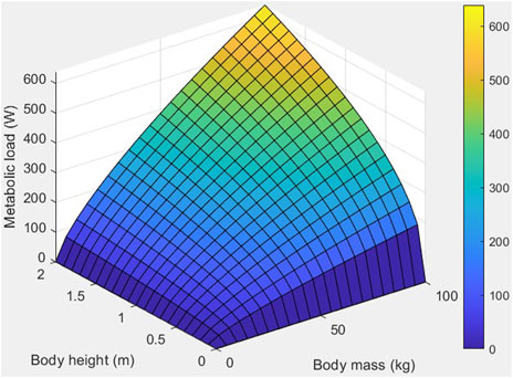
FIGURE 1. Metabolic heat load distribution vs. body mass (kg) and body height (m).

Figure 2 portrays the surface plot of the metabolic heat load distribution against the body surface area and the number of passengers. It can clearly be seen that the greater the number of passengers, the higher the metabolic heat dissipation into the cabin. Moreover, the plot shows that a larger body surface area coincides with a higher metabolic heat load. The factors highlighted in Figure 1 and Figure 2 should be taken into account when designing automotive AC systems.

FIGURE 2

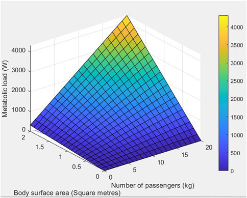
FIGURE 2. Metabolic heat load distribution vs. body surface area (m²) and number of passengers.

2.2 Modeling of ambient load

The ambient temperature affects the calculation of external and internal cooling loads of an automotive AC. The ambient load can be expressed as in Eq. 13.

$Q_{Amb}={\displaystyle \sum }_{i=1}^n{S}_{i}U\left(T_S-T_i\right)(13)$

In Eq. 13, $T_0$ denotes the average ambient temperature, $T_S$ denotes the average surface temperature, $T_i$ denotes the average cabin temperature, $S_i$ denotes the surface area of the vehicular body ($i^{th}$ surface), and $U$ denotes the overall heat transfer coefficient. When estimating the ambient load in the local context, the mean annual temperature in Sri Lanka was estimated to be 27.50°C (Department of Meteorology, 2017). As in Eq. 13, $T_i$ is determined by subtracting 5.00°C from the average ambient temperature, whereas $T_S$ is determined as stated in Eq. 15.

$T_i=T_0-5.00(14)$

$T_s=T_0+5.00(15)$

The term $U$ can be determined using the formula in Eq. 16 in terms of $R$, the net thermal resistance for a unit surface area. The overall heat transfer coefficient and the net thermal resistance for a unit surface area have an inversely proportional relationship as stated in Eq. 16.

$U=1/R(16)$

The R value can be determined using the formula shown in Eq. 17.

$R=\raisebox{1ex}{$1$}\!\left/ \!\raisebox{-1ex}{$h$}\right.+\raisebox{1ex}{$\mathrm{ƛ}$}\!\left/ \!\raisebox{-1ex}{$k$}\right..(17)$

In Eq. 17, $h$ is the convection coefficient, $k$ is the surface thermal conductivity, and ƛ is the thickness of the surface element. The convection coefficient, $h$, depends on the orientation of the surface and the air velocity. Here, the following calculation is used to estimate the convection heat transfer coefficient as a function of vehicle speed and the relationship is shown in Eq. 18.

$h=0.6+6.64\sqrt{v}.(18)$

In Eq. 18, the terms can be elaborated as follows: $h$ denotes the convection coefficient, $\overline{v}$ is the mean vehicular velocity of the respective driving cycle, and $k$ is the surface thermal conductivity. The $k$ value can be approximated as 45 W/K/m for the typically used steel type containing 0.05%–0.25% carbon steel. (Department of Meteorology, 2017) The ƛ value is the thickness of the sheet metal and typically ranges from 0.7 mm to 1.2 mm in LDV manufacturing 20]. Thus, the average thickness of the surface is taken as 1.0 mm for calculation purposes in the study.

The ambient load varies with respect to the air velocity along the vehicular surface. The air velocity can be considered similar to the vehicular speed considering the relative motion between them. For the different driving cycles depicted in Table 2, the average speed varies among them, and therefore, the ambient load changes respectively. Assuming that the average speed estimated by the worldwide harmonized light vehicle test procedure (WLTP) is 12.91 m/s, the $h$ value can be determined as shown in Table 1. When the determined values are then substituted in (Eqs 15, 16), the overall heat transfer coefficient, $U$, can be determined. Once the computed $U$ value is substituted in Eq. 12, the ambient load can be determined as shown in Eqs 19, 20 as follows:

$R=0.04+\frac{1\mathrm{x}{10}^{-3}}{45}$

$=4.0\mathrm{x}{10}^{-2}+2.2\mathrm{x}{10}^{-5}$

$=0.04.(19)$

$U=\frac{1}{\mathrm{R}}$

$=\frac{1}{0.04}$

$=25W{m}^{-2}{K}^{-1}.(20)$

When determining the ambient load, the surface areas of the vehicular exterior should be taken into account. In this study, the vehicular surface area was estimated using the mean vehicular surface area, $\overline{S}$, which was estimated to be around 102.50 ft² (9.52 m²) and ranged from 87 to 118 ft² (Secondskinaudio, 2015).

$Q_{Amb}=\overline{S}U\left(T_S-T_i\right)$

$Q_{Amb}=\left(9.52\right)\left(25\right)\left(T_0+5.00-\left[T_0-5.00\right]\right)$

${\mathit{Q}}_{\mathit{A}\mathit{m}\mathit{b}}=\mathbf{2,380.00}\mathit{W}(21)$

TABLE 2

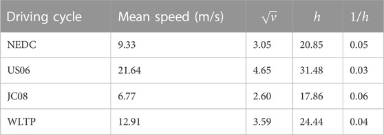
TABLE 2. Kinematic parameters for different driving cycles.

The ambient load of the A/C of an average passenger car can be estimated as 2,380 W as stated in Eq. 21, and it can be considered as a major contributor to the power demand of the A/C system.

The distribution of ambient heat load is clearly portrayed in the surface plot of Figure 3. The ambient heat load increases with increases in the temperature difference and the average speed of the vehicle. The ambient temperature difference signifies the temperature gap between the surface of the vehicular body and the cabin temperature.

FIGURE 3

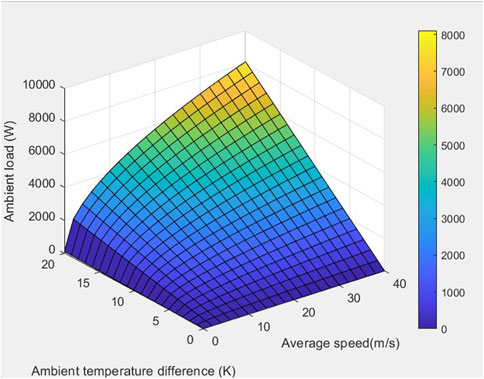
FIGURE 3. Ambient heat load distribution vs. average speed (m/s) and ambient temperature difference (K).

2.3 Modeling of radiation load

Radiation load is another key element in determining the total A/C load. The radiation load is comprised of three major components: direct radiation load, diffuse radiation load, and reflected radiation load. The direct radiation load is caused by the radiation of direct sunlight whereas diffuse radiation is that part of the solar radiation, which results from indirect daylight radiation on a surface. The reflected load is caused by the reflected radiation from the surfaces (Abdulsalam et al., 2007). The total radiation load can be modeled using the formula shown in Eq. 22 (Fayazbakhsh and Bahrami, 2013).

$Q_{Rad}=\frac{1}{2}S\alpha \left(I_{Dir}\mathit{Cos}\theta +I_{Dif}+I_{Ref}\right).(22)$

In Eq. 22, $Q_{Rad}$ denotes the total radiation load, $S$ is the surface area, $I_{Dir}$ is the direct radiation heat gain per unit area, $\theta$ is the angle between the surface normal and the position of the sun in the sky, $\alpha$ is the surface absorptivity, $I_{Dif}$ is the diffuse radiation heat gain per unit area, and $I_{Ref}$ is the reflected radiation heat gain per unit area. Considering the fact that solar radiation can affect only one particular half of the vehicle at a given time, a constant of ½ is added to (Eq. 22). When determining the radiation load, it’s important to obtain the position of the sun with respect to the earth.The mean altitude angle of sun, $\beta$, with respect to the earth during the mid-year can be determined as ˗30° (Solar elevation angle calculator, 2014).

$i_{Dir}=\frac{A}{e^{\raisebox{1ex}{$B$}\!\left/ \!\raisebox{-1ex}{$SinB$}\right.}}.(23)$

The direct radiation heat gain per unit area, i.e., $i_{Dir}$ can be determined using Eq. 23. Assuming the middle of the year, the constants $A$ and $B$ can be approximated as follows: $A$ = 1087.613 Wm^-2 and $B$ = 0.205 according to the ASHRAE Handbook of Fundamentals (ASHRAE, 2017). Substituting these $A$ and $B$ values in Eq. 23, the result shown in Eq. 24 is obtained.

$i_{Dir}=\raisebox{1ex}{$1087.613$}\!\left/ \!\raisebox{-1ex}{$e^{\left(\raisebox{1ex}{$0.205$}\!\left/ \!\raisebox{-1ex}{$\mathit{Sin}\left(-30\right)$}\right.\right)}$}\right.$

$=1087.613/0.6636$

$i_{Dir}=\mathbf{1,639}\mathbf{W},(24)$

$i_{Dif}=C\ast I_{Dir}\left(1+CosE\right)/2.(25)$

In Eq. 25, the constant $C$ can be approximated to 0.134 (ASHRAE, 2017). Assuming that $E$ equals 45°, then $i_{Dif}$ can be determined, and the result is shown in Eq. 26.

$i_{Dif}=\raisebox{1ex}{$\left(0.13\right)\left(1639\right)\left(1+0.71\right)$}\!\left/ \!\raisebox{-1ex}{$2$}\right.$

$i_{Dif}=\mathbf{187.45}\mathbf{W}(26)$

$I_{Ref}$ can be determined using the direct and diffuse radiation heat gain per unit area as in Eq. 27.

$i_{Ref}=\left(i_{Dir}+i_{Dif}\right)\ast {\rho }_g\left(1-CosE\right)/2(27)$

The term ${\rho }_g$ denotes the ground reflectivity coefficient, which ranges from 0.20 to 0.35 for rough surfaces (ITU -R). The mean ground reflectivity coefficient, $\overline{{\rho }_g}$, is assumed be 0.30. The $I_{Ref}$ value can then be determined using Eq. 27 and the result is given in Eq. 28 as follows:

$i_{Ref}=\left(1639+187.45\right)\ast 0.30\left(1-0.71\right)/2,$

$i_{Ref}=\mathbf{80.27}\mathit{W}.(28)$

The surface absorptivity value, $\alpha$, is approximated as 0.4 (Surface Absoptivity, 2016). Also, since $\theta$ is approximately 45°, $\mathit{Cos}\theta$ can be determined as 0.707.

${\mathrm{Q}}_{\mathrm{s}\mathrm{R}\mathrm{a}\mathrm{d}}=0.5\mathrm{x}9.52\mathrm{x}0.4\left(1639\mathrm{x}0.71+82.54+35.35\right)$

$\dot{{\mathit{Q}}_{\mathit{s}\mathit{R}\mathit{a}\mathit{d}}=}\mathbf{2,430.80}\mathit{W}(29)$

Therefore, the total radiation load comprised of direct, diffuse, and reflected radiation is determined as stated in Eq. 29, and it can be claimed as one of the highest contributors to the automotive AC load with a power requirement of around 2.43 kW. Moreover, it accounts for 24% of the automotive AC power demand. The automotive AC energy efficiency can be improved by finding ways to mitigate the impact of the radiation heat load.

2.4 Modeling of exhaust load

Since the study encompasses the scope of LDVs equipped with internal combustion engine (ICEs), exhaust emission is generated and transmitted from the exhaust manifold of the engine through the exhaust lines underneath the cabin to the tailpipe. The higher temperature of the exhaust gas can contribute to the thermal gain of the cabin through the cabin floor. The exhaust load can be modeled using the formula in Eq. 30.

$Q_{Exh}=S_{Exh}U\left(T_{Exh}-T_i\right).(30)$

In Eq. 30, $U$ denotes overall heat transfer coefficient, $S_{Exh}$ is the surface area exposed to heat from the exhaust gas (area in contact with the exhaust line), $T_{Exh}$ is the exhaust gas temperature, and $T_i$ is the cabin temperature.

In determining the average surface area exposed to exhaust heat, the following assumptions and calculations have been made. The length of an average car is assumed to be 15 feet (4.50 m) (Automobiledimension, 2018). The length of an average exhaust-line ($L_{Exh}$) is determined by multiplying the length of an average car by a factor of 0.75; thus, $L_{Exh}$ can be estimated as 3.38 m. The average diameter of the exhaust line, D, (for ≤2.5 L IC engine in a 300 bhp vehicle) can be estimated as 2.5 inches (63.5 × 10^–3 m). Assuming the area in contact with the exhaust line is the area of its projection on the bottom surface of the car, the relationship in Eq. 31 can be developed.

$S_{Exh}=L_{Exh}\mathrm{x}D=3.38\mathrm{x}63.5\mathrm{x}{10}^{-3}$

$=214.6\mathrm{x}{10}^{-3}{m}^2.(31)$

The average cabin temperature, $T_i$, can be approximated as $\left(T_0-5\right)$, whereas the overall heat transfer coefficient, $U$, can be approximated as 25 Wm⁻²K⁻¹. The exhaust gas temperature ($T_{Exh}$) can be estimated using the linear function of engine RPMs as stated in Eq. 32 (Gota, 2018).

$T_{Exh}=0.14RPM-17.(32)$

Approximating the normal operating RPM of a 4-stroke ICE as 3000 RPM, the $T_{Exh}$ can be determined as 403.0°C when substituted in Eq. 32.

$\dot{Q_{Exh}}=\left(214.60\ast {10}^{-3}\right)\ast 25\ast \left(403.00-22.50\right),$

${\mathit{Q}}_{\mathit{E}\mathit{x}\mathit{h}}=\mathbf{2,041.40}\mathbf{W}.(33)$

Consequently, as shown in Eq. 33, the average exhaust load of an automotive AC is determined to be 2 kW under local conditions.

2.5 Modeling of engine load

Engine load determines the amount of excess heat generated by the IC engine and the amount transferred into the cabin. The engine load can be modeled using the formula in Eq. 34.

$\dot{Q_{Eng}}=S_{Eng}U\left(T_{Eng}-T_i\right).(34)$

In Eq. 34, $S_{Eng}$ denotes the surface area exposed to engine temperature, $T_{Eng}$ is the engine temperature, and $T_i$ is the cabin temperature. The U value is estimated as 25 Wm⁻²K⁻¹. Assuming that the area exposed to engine temperature of an average car is defined by setting effective height = 0.5 x height, the value for $S_{Eng}$ is calculated as stated in Eq. 35.

$S_{Eng}=Tracklength\times Effectiveheight,$

$S_{Eng}=\left(1464\right){10}^{-3}\left(446.30\right){10}^{-3},$

$S_{Eng}=0.65m^2.(35)$

The estimation of the engine temperature can be performed using the formula in Eq. 36 (Khayyam et al., 2009).

$T_{Eng}=-2\ast {10}^{-6}{RPM}^2+0.04RPM+77.5$

$T_{Eng}=-2\ast {10}^{-6}\ast {3000}^2+0.04\ast 3000+77.5(36)$

$=-18.00+120.00+77.50$

$={179.50}^{0}C\left(theestimatedenginetemperatureundergivenconditions\right)$

The variation of engine load on par with engine RPM is depicted in Figure 4. It can be seen that the instantaneous engine heat load increases quadratically as a function of engine RPM.

$\dot{Q_{Eng}}=S_{Eng}U\left(T_{Eng}-T_i\right)$

$\dot{Q_{Eng}}=0.65*25\left(179.50-22.50\right)$

$\dot{{\mathit{Q}}_{\mathit{E}\mathit{n}\mathit{g}}}=\mathbf{2551.25}\mathit{W}(37)$

FIGURE 4

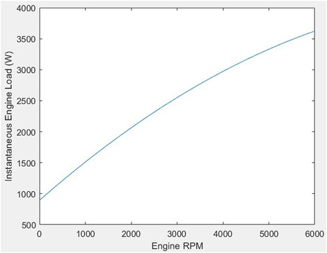
FIGURE 4. Engine load vs. engine RPM.

Consequently, the engine load can be determined as stated in Eq. 37, using the aforementioned steps. The average engine load can be approximated as 2.6 kW under the given conditions.

2.6 Modeling of ventilation load

Due to the leakage of air within the cabin to the atmosphere, ambient air is assumed to enter the cabin at the ambient temperature and with higher relative humidity. Typically, once steady-state operation is reached, the cabin air pressure is greater than the ambient air pressure. The thermal load can then be determined using the formula in Eq. 38 (Abdulsalam et al., 2007):

$\dot{Q_{Ven}}=\dot{m_{ven}}\left(e_o-e_i\right)(38)$

In Eq. 38, $e_o$ denotes ambient enthalpy, $e_i$ is cabin enthalpy, and $\dot{m_{ven}}$ is ventilation mass flow rate. The formula used to determine the enthalpy ($e$) is stated in Eq. 39 (Abdulsalam et al., 2007).

$e=1006T+\left(2.501\ast {10}^6+1770T\right)\overline{X.}(39)$

In Eq. 39, $T$ denotes mean air temperature, $\overline{X}$ is mean humidity ratio in grams of dry air, and $\overline{X}$ can be modeled using the formula stated in Eq. 40.

$\overline{X}=0.62\frac{\varnothing P_s}{100P-\varnothing P_s}.(40)$

In Eq. 40, $\varnothing$ (relative humidity) is approximated as 74.0%, $P_s$, the ambient saturated vapor pressure, is estimated as 3693.03 Pa, and $P$, the atmospheric pressure, is estimated as 1001.00 mbar = 1.00100 × 10⁵ Pa in reference to the local geography of Colombo, Sri Lanka.

$\overline{X}=0.62\frac{0.74\ast 3693.03}{100\ast 1.001\ast {10}^5-0.74\ast 3693.03}$

$\overline{X}=0.62\frac{2732.84}{1.01\ast {10}^7},$

$\overline{X_{Amb}}=1.68\ast {10}^{-4}\mathrm{g}\left(\mathrm{a}\mathrm{m}\mathrm{b}\mathrm{i}\mathrm{e}\mathrm{n}\mathrm{t}\overline{\mathrm{X}}\mathrm{v}\mathrm{a}\mathrm{l}\mathrm{u}\mathrm{e}\right)(41)$

The saturated vapor pressure and the relative humidity values should be substituted in (40) in reference to the values portrayed in Table 3.

TABLE 3

TABLE 3. Relative humidity (RH) and saturated vapor pressures at given temperatures.

After substituting the ambient values into Eq. 40, the value in Eq. 41 can be obtained. Similarly, for cabin parameters, Eq. 42 can be obtained.

$\overline{X}=0.62\frac{0.50*2980.04}{100\ast 1.001\ast {10}^5-0.50\ast 2980.04}$

$\overline{X_{Cabin}}=0.93*{10}^{-4}\left(\overline{X}\mathrm{w}\mathrm{i}\mathrm{t}\mathrm{h}\mathrm{i}\mathrm{n}\mathrm{t}\mathrm{h}\mathrm{e}\mathrm{c}\mathrm{a}\mathrm{b}\mathrm{i}\mathrm{n}\right)(42)$

According to the local context, $\overline{X}$ = 74.0%; $T$ = 27.5°C (Allen and Lasecki, 2001) and substituting the respective values into Eq. 39, the result in Eq. 43 can be obtained.

$e_o=1006\left(273.15+27.50\right)+\left(2.501*{10}^6+1770\left[273.15+27.50\right]\right)\left(1.682*{10}^{-4}\right),$

$e_o=0.303*{10}^6+2.501*{10}^6,$

$e_o=0.304*{10}^{6}J(43)$

It is assumed that the mean RH of an air-conditioned car is around 50% [range, 30% to 65%, for temperatures from 20–25°C].

$e_i=1006\left(273.15+22.50\right)+\left(2.501*{10}^6+1770\left[273.15+22.50\right]\right)\left(0.926*{10}^{-4}\right),$

$e_i=0.299*{10}^6+2.501*{10}^6,$

$e_i=0.298*{10}^{6}J(44)$

Similar to the method for obtaining (43), the result in Eq. 44 was achieved by assuming a mean mass air flow rate of 0.02 m³s^-1, allowing the ventilation load to be determined as stated in Eq. 45.

$\dot{m_{ven}}=0.02m^3{s}^{-1},$

$\dot{Q_{Ven}}=0.02\left(0.304-0.298\right)*{10}^6,(45)$

$\dot{{\mathit{Q}}_{\mathit{V}\mathit{e}\mathit{n}}}=\mathbf{120.00}\mathit{W}.$

Consequently, the average ventilation load of an automobile is estimated under the given local conditions as 120 W, which is comparatively lower than the other AC loads. Lastly, a summary of the determined values for each type of AC load under local conditions is provided in Table 4.

TABLE 4

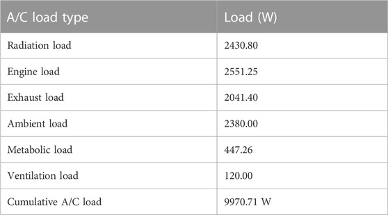
TABLE 4. A/C load breakdown.

3 Estimating the power demand of an automotive alternator

Alternators are the primary source of electric energy within a vehicle. The electric power demand of a contemporary automobile has rapidly increased along with the increase in use of electrical devices. The alternator provides the electric output as a consequence of an energy conversion chain. Taking the average efficiency values into account, the internal combustion engine has an efficiency of 40%, the belt-drive has an efficiency of 98%, and the alternator has an efficiency of 55%, which leads to an overall energy efficiency of around 21% (Allen and Lasecki, 2001).

Simply stated, an alternator is a synchronous alternating current (AC) electric generator with direct current (DC) diode rectification and pulse-width modulation voltage control (SAE International, 2011). It consists of a rotor, stator, diode rectifier, and voltage regulator. An automotive alternator has an efficiency of about 55% at an operating RPM of 1500. The power loss in an alternator is another important aspect to be analyzed since it can contribute to increased fuel consumption. The losses can be classified into three main types: electrical, magnetic, and mechanical. With this in mind, the overall energy conversion efficiency of an alternator can be stated as:

$\eta =\frac{P_{Out}}{P_{In}}.(46)$

In Eq. 46, $\eta$ is the overall alternator efficiency, $P_{In}$ is the input mechanical power, and $P_{Out}$ is the output electrical power. The value of $\eta$ can then be expressed as shown in Eq. 47:

$\eta =\frac{P_{Out}}{P_{Out}+P_{Losses}}.(47)$

It can be stated that the peak efficiency of an automotive alternator lies around 55% at an operating RPM of around 1500 (Liaw et al., 2006; Gajanayake et al., 2020). The term, $P_{Losses}$, in Eq. 47 denotes the aggregated power losses within the alternator. The typical voltage output of an automotive alternator in a 12-V vehicle electric system is 13.8–14.3 V. Assuming that the peak amperage of the alternator at 14.0 V is 110.0 A at 1500 RPM, the input mechanical power demand of an alternator with 55% overall efficiency can be expressed as follows(Eq. 48):

$P_{Out}=V_{out}*I_{Out},$

$P_{Out}=14.0*110.0,(48)$

$P_{Out}=1540.0\mathrm{W}.$

Assuming an alternator efficiency, $\eta$, of 55%, then the average power demand of an alternator can be determined as stated in Eq. 49:

$\eta =\frac{P_{Out}}{P_{In}},$

$P_{In}=\frac{P_{Out}}{\eta },$

$P_{In}=\frac{1540}{0.55},$

${\mathit{P}}_{\mathit{I}\mathit{n}}=\mathbf{2,800.0}\mathrm{W}.(49)$

Therefore, the average input power demand of an automotive alternator is 2.8 kW, which is a significantly higher contributor.

4 Estimating the power demand of other engine auxiliaries

In this study, the mechanical water pump and the power steering pump were identified and studied as auxiliary devices that run by engine power in addition to the AC and the alternator. When estimating the power demand of the water pump and the power steering pump, previous literature has been critically appraised. First, the power demand of the water pump is discussed and estimated. During driving cycle test schedules, which run from 1200 to 1800 s, the operation of the cooling system of an internal combustion engine (ICE) is critically important to ensure that the engine remains within the optimum operating temperature range. ICEs account for many types of heat losses, and the water pump is an essential device for circulating the coolant fluid within the engine block to maintain an optimum temperature. Every vehicle equipped with an ICE has a water pump that is operated either mechanically or electrically. In this study, the mechanical version of the water pump will be discussed. It operates as an engine auxiliary load that is coupled to the engine crankshaft by a serpentine belt. Single-stage radial centrifugal pumps are used in the vast majority of motor vehicle cooling circuits, and the speed of the pump and coolant flow rate are linked directly to the engine speed.

A typical mechanical water pump consists of an impeller located inside a spiral housing and sealed by an axial face seal. The spiral housing is mounted to the engine block with ports leading into and out of the coolant fluid channels within the engine block. The mechanical power arrives through the hub with a pulley. The channels on the pulley indicate the interface for the guides on the serpentine belt which transmits power from the crankshaft (Wang et al., 2015b). When referring to the relationship of the pressure generated within the water pump and the respective flow rate at different engine speeds, it can be seen that as the in the engine speed increases, the pump pressure also increases (Gota, 2018). Consequently, the amount of fluid horsepower generated will also be increased. The mechanical efficiency of a water pump typically lies between 35% and 55% for engine speeds ranging from 1000 RPM (idle) to 5000 RPM (Allen and Lasecki, 2001). The input power required by the water pump varies from 185 W to 220 W depending on the RPM range from 3000–5000 RPM. For an operating RPM of 3000, the power demand of the water pump can be estimated at 185 W.

The power steering pump is the other type of engine auxiliary for which the power demand was estimated and discussed in this study. During the driving cycle tests, the lateral motion of the vehicle steering was not considered; only the power demand of the power steering pump during the course of straight driving was discussed. When considering power steering mechanisms, there are two main technologies used: hydraulic power-assisted steering (HPAS) and electronic power-assisted steering (EPAS). The power consumption during a straight driving course shows significant discrepancies between these two technologies. The studies of Herkommer (Herkommer, 2002) have determined that fuel consumption was reduced up to 0.25 L per 100 km when EPAS systems were introduced in LDVs. In the conventional HPAS system, the power demand is dependent upon the delivery of oil and the system consumes approximately 0.3 L of fuel per 100 km (Herkommer, 2002) (Breitfeld et al., 2002).

Hydraulic pumps are usually fix-mounted to the engine and connected to the crankshaft by the serpentine belt. Since the engine RPM varies during driving, the flow delivered by the pump also varies proportionally, but the pumps are designed to deliver full flow at idle speed. This leads to the production of surplus oil when the engine runs at operating RPM, and this surplus oil is accountable for most of the power consumption associated with HPAS. Therefore, it is somewhat surprising that the overall energy efficiency of the HPAS system, 60%, is quite a lot higher than that of the EPAS system, at 22% (Wang et al., 2015b). The greater number of levels of power transmission in the EPAS system relative to the HPAS system is the cause of the lower efficiency values. Despite the lower efficiency, the overall power demand of the EPAS system is significantly lower than that of the HPAS system. The EPAS system is accountable for an overall power demand of approximately 38.5 W, whereas the HPAS system has an overall power demand of 175 W.

5 Conclusion

Auxiliary engine components play a significant role in contributing to the engine power demand. The percentage contributions of each auxiliary load toward the engine power demand are given as in Table 5.

TABLE 5

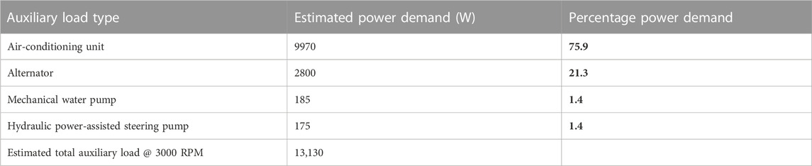
TABLE 5. Summary of engine auxiliary power demand.

Almost all the auxiliary equipment discussed in the study is belt-driven, and thus, there’s a significant dependency on engine speed and subsequently on the vehicular speed as well. Therefore, when tested on a driving cycle, the auxiliary equipment has a significant impact on the operating fuel economy of a light duty vehicle.

When analyzing the belt-driven mechanical auxiliary loads of the A/C unit, alternator, water pump, and steering pump, we found that the major users of engine power were the A/C system and the alternator, accounting for more than 97% of the total auxiliary power requirement. The power demands of the water pump and the power steering pump are quite low, around 3% of the total auxiliary power demand. When determining the auxiliary power requirements, an operating RPM of 3,000 was assumed, whereas the other physical factors were considered with respect to the local Sri Lankan context. For a standard LDV with a rated engine power of 100 bhp, equivalent to 74.7 kW, the engine auxiliaries required about 13.130 kW, which accounted for 17.6% of the engine’s total rated power. Therefore, it can be concluded that auxiliary engine loads must be taken into account when modeling the overall engine power demand since they claim a substantial portion of engine power and should be considered a main factor in modeling the engine loads on par with tractive loads and other inertial engine loads.

Data availability statement

The original contributions presented in the study are included in the article/Supplementary Material; further inquiries can be directed to the corresponding author.

Author contributions

All authors listed have made a substantial, direct, and intellectual contribution to the work and approved it for publication.

Conflict of interest

The authors declare that the research was conducted in the absence of any commercial or financial relationships that could be construed as a potential conflict of interest.

Publisher’s note

All claims expressed in this article are solely those of the authors and do not necessarily represent those of their affiliated organizations, or those of the publisher, the editors, and the reviewers. Any product that may be evaluated in this article, or claim that may be made by its manufacturer, is not guaranteed or endorsed by the publisher.

References

Abdulsalam, O., Santoso, B., and Aries, D. (2007). Cooling load calculation and thermal modeling for vehicle by MATLAB. Int. J. Innovative Res. Sci. Eng. Technol. 3297 (5), 3052–3060. doi:10.15680/IJIRSET.2015.0405076

CrossRef Full Text | Google Scholar

Allen, D. J., and Lasecki, M. P. (2001). Thermal management evolution and controlled coolant flow. Technical Paper Series 2001-01-1732. Society of Automobile Engineers.

Google Scholar

ASHRAE (2017). Hvac system design software. 2nd. Ashrae. Available at: http://www.carrier.com/commercial/en/us/software/hvac-system-design/.

Google Scholar

Automobiledimension (2018). Body dimensions. Available at: https://www.automobiledimension.com/ (Accessed June 20, 2021).

Google Scholar

Bradfield, M. (2008). Improving alternator efficiency measurably reduces fuel costs 1–31. Indiana, United States: Remy International Inc.

Google Scholar

Breitfeld, C., Foag, W., Guldner, J., M¨uller, S., Schmidt, W., and Vielwerth, G. (2002). “Actuator principles for integrated chassis control system - a comarison,” in 3rd International Fluid Power Conference, Aachen, Germany, March 2002, 399–418. ISBN 3–8265–9900–4. 42V.

Google Scholar

Cho, G., Wi, H., Lee, J., Park, J., and Park, K. (2008). Effect of alternator control on vehicle fuel economy. Trans. KSAE 17 (2), 20–25.

Google Scholar

Cuma, M. U., and Koroglu, T. (2015). A comprehensive review on estimation strategies used in hybrid and battery electric vehicles. Renew. Sustain Energy Rev. 42, 517–531. doi:10.1016/j.rser.2014.10.047

CrossRef Full Text | Google Scholar

Department of Meteorology (2017). Department of Meteorology. Available at: https://www.meteo.gov.lk (Accessed July 25, 2021).

Google Scholar

Fayazbakhsh, M. A., and Bahrami, M. (2013). Comprehensive modeling of vehicle air conditioning loads using heat balance method. SAE Tech. Pap. 2, 2688–3627. doi:10.4271/2013-01-1507

CrossRef Full Text | Google Scholar

Gajanayake, S., Thilakshan, T., Sugathapala, T., and Bandara, S. (2020). “Study of the impact of electric vehicles on fuel consumption and carbon dioxide emission scenarios in Sri Lanka” in 2020 Moratuwa Engineering Research Conference (MERCon), 494–498. doi:10.1109/MERCon50084.2020.9185248

CrossRef Full Text | Google Scholar

Gota, S. (2018). Two-and-Three-Wheelers: A policy guide to sustainable mobility solutions for motorcycles 40. Available at: https://www.sutp.org/files/contents/documents/resources/A_Sourcebook/SB4_Vehicles-and-Fuels/GIZ_SUTP_TUMI_SB4c_Two- and Three-Wheelers_EN.pdf.

Google Scholar

Hara, D., and Özgen, G. O. (2016). Investigation of weight reduction of automotive body structures with the use of sandwich materials. Transp. Res. Procedia 14, 1013–1020. doi:10.1016/j.trpro.2016.05.081

CrossRef Full Text | Google Scholar

Havenith, G., Holmér, I., and Parsons, K. (2002). Personal factors in thermal comfort assessment: Clothing properties and metabolic heat production. Energy Build. 34, 581–591. doi:10.1016/S0378-7788(02)00008-7

CrossRef Full Text | Google Scholar

Herkommer, R. (2002). “Ways toward energy saving in hydraulic steering system,” in 3rd International Fluid Power Conference, Aachen, Germany, March 2002, 465–474. IFK02, ISBN 3–8265–9900–4.

Google Scholar

ISO (1989). ISO 8996, ergonomics of thermal environments – determination of metabolic heat production. Geneva: ISO.

Google Scholar

ITU-R (1990). Reflection from the surface of the earth. Report P.1008-1.

Google Scholar

Khayyam, H., Kouzani, A. Z., and Hu, E. J. (2009). “Reducing energy consumption of vehicle air conditioning system by an energy management system,” in 2009 IEEE Intelligent Vehicles Symposium, Xi'an, China, 03-05 June 2009.

CrossRef Full Text | Google Scholar

Liaw, C., Whaley, D., Soong, W., and Nesimi, E. (2006). Investigation of inverter less control of interior permanent-magnet alternators. IEEE Trans. Ind. Appl. 42 (2), 536–544. doi:10.1109/TIA.2005.863910

CrossRef Full Text | Google Scholar

Martinez, R., Zhou, B., Sophiea, M. K., Bentham, J., Paciorek, C. J., Iurilli, M. L., et al. (2020). Height and body-mass index trajectories of school-aged children and adolescents from 1985 to 2019 in 200 countries and territories: A pooled analysis of 2181 population-based studies with 65 million participants. Lancet 396 (10261), 1511–1524. PMC 7658740. PMID 33160572. doi:10.1016/S0140-6736(20)31859-6

PubMed Abstract | CrossRef Full Text | Google Scholar

Nadamoto, H., and Kubota, A. (1999). Power saving with the use of variable displacement compressor. Technical Paper1999- 01-0875. Society of Automobile Engineers.

Google Scholar

Patel, B. M., Modi, A. J., and Rathod, P. P. (2013). Analysis on engine cooling water pump of car and significance of its geometry. Intl. J. Mech. Eng. Technol. 4 (3), 100–107. ISSN 0976–6340.

Google Scholar

Roskilly, A. P., Palacin, R., and Yan, J. (2015). Novel technologies and strategies for clean transport systems. Appl. Energy 157, 563–566. doi:10.1016/j.apenergy.2015.09.051

CrossRef Full Text | Google Scholar

SAE International (2011). Automotive Handbook. 8th Edition. Plochigen: Robert Bosch, 952–968.

Google Scholar

Secondskinaudio (2015). What's the square footage of my vehicle? Available at: https://www.secondskinaudio.com/square-footage-help/ (Accessed July 29, 2021).

Google Scholar

Solar elevation angle Calculator (2014). Solar elevation angle (for a day) Calculator. Available at: https://keisan.casio.com/exec/system/1224682277 (Accessed October 2, 2021).

Google Scholar

Surface Absoptivity (2016). Resources, tools and basic information for engineering and design of technical applications. Available at: https://www.engineeringtoolbox.com/radiation-surface-absorptivity-d_1805.html (Accessed August 2, 2021).

Google Scholar

Tasuni, M. L. M., Latiff, Z. A., Nasution, H., Perang, M. R. M., Jamil, H. M., and Misseri, M. N. (2016). Performance of a water pump in an automotive engine cooling system. J. Teknol. 78 (10–2), 47–53.

Google Scholar

Wang, X., Liang, X., Hao, Z., and Chen, R. (2015). Comparison of electrical and mechanical water pump performance in internal combustion engine. Int. J. Veh. Syst. Model. Test. 10 (3), 205–223. doi:10.1504/IJVSMT.2015.070155

CrossRef Full Text | Google Scholar

Wang, X., Liang, X., Hao, Z., and Chen, R. (2015). Comparison of electrical and mechanical water pump performance in internal combustion engine. Int. J. Veh. Syst. Model. Test. 10 (3), 205–223. doi:10.1504/IJVSMT.2015.070155

CrossRef Full Text | Google Scholar

Welstand, J., Haskew, H., Gunst, R., and Bevilacqua, O. (2003). Evaluation of the effects of air conditioning operation and associated environmental conditions on vehicle emissions and fuel economy. Technical Paper 2003-01-2247. Society of Automobile Engineers.

Google Scholar

Weldon, P., Morrissey, P., and O'Mahony, M. (2016). Environmental impacts of varying electric vehicle user behaviours and comparisons to internal combustion engine vehicle usage–An Irish case study. J. Power Sources 319, 27–38. doi:10.1016/j.jpowsour.2016.04.051

CrossRef Full Text | Google Scholar

WHO (2015). Non-communicable disease risk factor survey Sri Lanka. (PDF). Sri Lanka: World Health Organization, 81.

Google Scholar

Wu, X. K., Freese, D., Cabrera, A., and Kitch, W. A. (2015). Electric vehicles’ energy consumption measurement and estimation. Transp. Res. D. Transp. Environ. 34, 52–67. doi:10.1016/j.trd.2014.10.007

CrossRef Full Text | Google Scholar

Zhang, Z., Wang, J., Feng, X., Chang, L., Chen, Y., and Wang, X. (2018). The solutions to electric vehicle air conditioning systems: A review. Renew. Sustain. Energy Rev. 91, 443–463. doi:10.1016/J.RSER.2018.04.005

CrossRef Full Text | Google Scholar

Zhaogang, Q. (2014). Advances on air conditioning and heat pump system in electric vehicles – a review. Renew. Sustain. Energy Rev. 38, 754–764. doi:10.1016/j.rser.2014.07.038

CrossRef Full Text | Google Scholar

Nomenclature

$Q_{Total}$ total air conditioning load

$Q_{Met}$ metabolic heat load

$Q_{Rad}$ radiation heat load

$Q_{Amb}$ ambient heat load

$Q_{Exh}$ exhaust heat load

$Q_{Eng}$ engine heat load

$Q_{Ven}$ ventilation heat load

$Q_{Sensible}$ sensible heat load

$Q_{Latent}$ latent heat load

$M_{Sensible}$ sensible metabolic heat production rate

$M_{Latent}$ latent metabolic heat production rate

$A_{Du}$ estimation of body surface area using Du Bois method

$W$ body mass

$H$ body height

${\overline{A}}_{DU}$ mean body surface area

$S_i$ surface area of the vehicular body ($i^{th}$ surface)

$T_i$ average cabin temperature

$T_S$ average surface temperature

$T_0$ average ambient temperature

$U$ overall heat transfer coefficient

$R$ net thermal resistance per unit surface area

$h$ convection coefficient

$\mathrm{ƛ}$ thickness of the surface element

$\overline{v}$ mean vehicular speed of the respective driving cycle

$\alpha$ surface absorptivity

$S$ surface area

$I_{Dir}$ direct radiation heat gain per unit area

$I_{Dif}$ diffuse radiation heat gain per unit area

$I_{Ref}$ reflected radiation heat gain per unit area

$\theta$ the angle between the surface normal and the position of the sun

$A,B,C-$ constants as per ASHRAE standards

${\rho }_g$ ground reflectivity coefficient

$\overline{{\rho }_g}$ mean ground reflectivity coefficient

$E$ orientation angle between the surface normal and the position of sun in the sky of sun w.r.t earth

$S_{Exh}$ surface area exposed to exhaust gas temperature

$T_{Exh}$ exhaust gas temperature

$L_{Exh}$ length of an average exhaust line

D the average diameter of the exhaust line

$S_{Eng}$ surface area exposed to engine temperature

$T_{Eng}$ engine temperature

$\dot{m_{ven}}$ ventilation mass flow rate

$e_o$ ambient enthalpy

$e_i$ cabin enthalpy

$\overline{X}$ mean humidity ratio in grams of dry air

$T$ mean air temperature

$ø$ relative humidity

$P_s$ ambient saturated vapor pressure

$P$ atmospheric pressure

$\eta$ overall alternator efficiency

$P_{In}$ input mechanical power

$P_{Out}$ output electrical power

$P_{Losses}$ aggregated power losses within the alternator

$V_{out}$ output voltage

$I_{out}$ output current

Abbreviations

A/C air conditioning

AC alternating current

ASHRAE American Society of Heating Refrigerating and Air-conditioning Engineers

BEVs battery electric vehicles

DC direct current

EPAS electronic power-assisted steering

EVs electric vehicles

HEVs hybrid electric vehicles

HPAS hydraulic power-assisted steering

ICE internal combustion engine

ISO International Organization for Standardization

JC08 Japanese Chassis Dynamometer Test Cycle

NEDC New European Driving Cycle

RH relative humidity

US06 United States Supplemental Federal Test Procedure

WLTP World Harmonized Light Vehicle Test Procedure