Method for predicting dynamic loads for a health monitoring system for subway tracks

Introduction

The railroad substructure absorbs the majority of the dynamic loads. Although there are different ambiance dynamic loads (either wind loads or seismic loads), the main load is caused by the train’s traffic. There are two types of substructure: on the ground and elevated structures or bridges. The dynamic response of each one is different, and in the case of bridge structures, it depends on the structural design. Recently there have been a few bridge failures, but many of the railroad systems in the world were built a long time ago. Therefore, it is mandatory to predict the bridges’ remaining life. Smith (Smith, 2005) described the different fatigue failures in railroads. Although fatigue analysis in railroads is well-known (more than 200 years of research), dramatic accidents still occur. Smith described the various fatigue failures in the wheel-rail interfaces: The failures related to the interface appear in the wheels, the rails, and the rail welds.

The dynamic behavior of the railcar depends on the wheel-rail interfaces. The failures related to the dynamic forces produced by the rotating systems and train velocity appear in the bearings, axles, gearboxes, bogies, suspension, breaks, rail fastenings, track foundation, and substructure. This classification avoids the inclusion of environmental cases.

The dynamic loads on the wheel-rail interaction are complex due to the stresses present in the contact area and the dynamic parameters. The dynamic loads are incremented by discontinuities and flexibility changes in the rail, damping of the ballast, and deformations on the base structure. Also, spalling on the rails and polygonising of the wheels are other sources of high-frequency dynamic loads. Koc et al. (2018) (Koç et al., 2021; Koç & Esen, 2017) modeled the vehicle-structure-road coupled interaction considering structural flexibility, vehicle parameters and road roughness.

Smith emphasized the need for more measurement technology and analysis technics to evaluate the dynamic loads’ evolution in the wheel-rail interaction.

Ngamkhanong et al. (2018) presented a review of the descriptions of the wheel-track interactions. They explained that the train dynamics and the elastic response of the substructure have complex behavior. Fermér & Nielsen, 1995 presented an experimental and analytical work. They considered the wheel’s deformations and estimated the track parameters based on frequency analyses. The most accepted model assumes that the rail behaves as a beam and the sleepers as individual springs. Farmer and Nielsen represented the rail profile as an external excitation. Ciotlaus et al. (2019) described the wheel-track interaction considering that the contact occurs at a line, and they developed a model based on the rolling contact, fatigue, and wear.

Another dynamic source is the phenomenon known as hunting. Hunting is a swaying motion (lateral direction) of the train caused by the coning action. Zhai & Wang, 2010 incorporated the time history to model critical hunting speed. According to their work, most models only consider rigid elastic track, but they claimed that the track has a viscoelastic behavior. An experimental rig was developed by Naeimi et al. (2014). The wheel-track contact was represented as parabolic, and they assured that the scale model had the same pressure stresses as the original system. Similarly, other researchers have analyzed the dynamic interaction to determine predicting models for different operating conditions (Shi et al., 2021).

The measurements of wheel-track interaction are only possible with a complex instrumentation setup and sophisticated data analysis. Several publications reported modeling the structure, determining the wheel-track forces, specific test rigs, and data analysis. Quirke et al. presented a method for detecting bridges’ damages by sensing the traffic flow (Quirke et al., 2017). Weston et al. (2015). defined a procedure for observing track degradations that can be used for maintenance decisions. Chen & Fang, 2019 presented a method for predicting the train-track interaction; they made a numerical model of the interaction and found that the track deformation showed a similar waveform as the experimental results described in the following sections.

Usman, Burrow, and Ghataora (Usman et al., 2015) describe the failure mechanism in the subgrade. The failures are induced by climate changes that soften the subgrade. They developed a fault tree analysis. The substructure stiffness depends on the flexibility of the steel structure and the trackbed layers. They described that the failure in the sub-structure is related to the dynamic loads induced by the train and the modifications on the sub-structure by environmental changes (degradation of the trackbed layers, displacements on the bridge structure due to seismic loads). The ballast suffers from attrition due to the train’s dynamic load. Liu et al., 2020 described a method for detecting failures in welded joints on railway systems. They developed a detector that identifies defects on the welded joints through image processing and an intelligent algorithm. Inspection is either visual or instrumented, and it needs expert technicians and extended periods. Instrumented inspection utilizes cameras and ultrasonic sensors. Their method is based on a deep learning algorithm.

Hoang et al., 2020 presented the development of a wireless sensor for monitoring railroad bridges. Some of the problems with tracking bridges’ dynamic loads are recording a large amount of data and the ability of the wireless system to transmit them. They used appropriate algorithms, especially for the duration of the train on the bridge and data recovery and transmitting processed data to the operator. Thompson (Thompson, 2014) presented work on noise and vibration on the railroad. He described the vibration sources (rail cracks, track settlement, hanging sleepers, wear, and hunting) and the effect of the wheel’s circular frequency.

Other studies characterized the effect of vehicle traffic on the health of bridges. Different analysis techniques were applied for determining the relationship between the vehicle accelerations and the bridge strains. Such as the measurement of dynamic strains and accelerations on the foundation (Davis & Sanayei, 2020). Other studies were based on modeling the vehicle interaction with the bridges structure and substructure (Esen, 2011; Mizrak & Esen, 2015; Pehlivan et al., 2018) (Daniel & Kortiš, 2017),. Malekjafarian et al. (2019) and (Malekjafarian & OBrien, 2017) applied accelerometers and GPS for monitoring track conditions. Several works described the correlation between track’s profile and train’s acceleration (Dumitriu & Gheţi, 2019), (Molodova et al., 2016), (Entezami & Shariatmadar, 2019), (Cantero et al., 2019), and (Chang et al., 2019). These models included the local deformation (Hertz deformation), friction, and the dynamic loads produced by the vehicle over the track.

The health monitoring systems are the source for the maintenance of railroad programs. Among the primary methods for maintaining the railway infrastructure are monitoring the assets and the track condition monitoring (Turner et al., 2016). The subway operators require intelligent systems to predict and prognosis railway failures. These intelligent systems must include data acquisition systems, models for predicting the health condition based on the evolution of the data acquired, prognostic information, online reports of the health condition, and an alarm system to anticipate possible failures.

The interaction train-track depends on the vehicle dynamics and the friction force between the wheel and the track. Jaschinski et al. (1999) described the dynamic interaction analysis with scaled models because the dynamic response depends on the system and its influence on the measurements. They recommended scaling the system, considering that the original and scaled models have the same natural frequencies. Another important aspect is the number of degrees of freedom; they recommended that the scaled and original models have the same number of degrees of freedom. The primary consideration was that the scaled model represented similarity with the parameters that are being studied. Akutagawa & Wakao, 2018 defined vehicle scaling by relating the torque and the tracking force. There is a critical relationship that determines the slipping conditions at the wheel. Other researchers have analyzed the effect of scaling the dynamic behavior of vehicles; there are different factors and criteria to scale the model; some criteria are based on Buckingham’s theorem.

Although the dynamic wheel-track interaction is being widely studied, finding the location of possible failures along the track is very cumbersome. On the other hand, the easiest way of determining the train’s dynamic behavior is by measuring the accelerations along an entire track; nevertheless, the analysis and interpretation of the data are problematic. This paper presents a procedure for converting acceleration data into track deformations (loads). The procedure consists of finding a transfer function between the acceleration data and deformations (strains) measured at different locations on the track. With this procedure, the acceleration data obtained during the train’s operation can be converted into local deformations on the entire track. The deformation data give better information on the actual loading than the acceleration data; thus, it better reflects the damage evolution on the track and substructures. The transfer function was developed using an experimental rig, and afterward, it was applied to an existing Subway system.

The following section describes a transfer function that relates the strains on the track with the accelerations of a railcar. The following section describes the application of the transfer function to a subway system.

Force estimation

Experimental procedure

A particular scaled-down experimental facility was constructed to measure a railcar’s dynamic effect over the track (the scale ratio is 1/10). The testing facility had a flat table supporting the track and a mechanism for changing the inclination of the table. The railcar ran freely on the track, while the inclination angle determined the railcar’s acceleration and maximum speed, with normal forces exerted on the track. The vehicle speed depended on the friction coefficient (Romero Navarrete & Otremba, 2020). The railcar imposed forces in three orthogonal directions, the straight section accelerated the railcar (forward), and the lateral force was increased with a 180° curve.

The speed was measured with an optical sensor mounted on the railcar. The acceleration was measured with six degrees of freedom MEMS accelerometers (three orthogonal accelerations and three gyroscopes). The gravity component on the vertical was eliminated, and it was insignificant in the other two directions (lateral and longitudinal). The sample rate was 1,594 Hz. The railcar had a spring suspension, and the wheelbase was 150 mm. The track deformation was measured with strain gauges along the track; the strain gauges were aligned perpendicular to the wheel’s cone surface (Figure 1). The rail gap was the trigger for synchronizing the deformations and acceleration measurements. The strain gauge resistance was 120 ohms with a quarter-bridge connection, and the sample rate was 2,400 Hz.

FIGURE 1

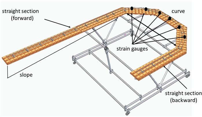
FIGURE 1. Sketch representing the track and the support structure.

The data contained all the acceleration and force measurements from the beginning of the railcar motion until it stopped. Two tests were conducted; the first type consisted of impact tests to determine the railcar’s and track natural frequencies. The second type was the running test. It consisted of letting the train run freely and simultaneously recording the train’s accelerations and track deformations.

Results

The data analysis began with identifying the natural frequencies of the railcar mounted on the track (impact test). The railcar was hit with a hammer, and the accelerometers recorded the dynamic response. This paper only includes the orthogonal accelerations’ response since they are the basis for estimating the transfer function between the railcar and track dynamic deformation. Table 1 lists the three main natural frequencies. The X-direction corresponds to the direction of motion, the Y-direction to the lateral movement, and the Z-direction to the vertical motion. The track deformation depends on the dynamic loads along with the three directions. Therefore, the transfer function considers the contribution of the three components, especially along a curve. These values were used for the Empirical Mode Decomposition (EMD) analysis.

TABLE 1

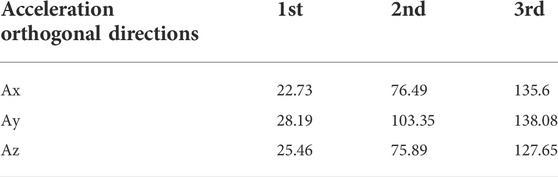
TABLE 1. Railcar’s natural frequencies (Hz).

The running test consisted of realizing the railcar at the highest point and stopping at the curve’s end (Figure 1). The data were recorded during the entire railcar’s path. The results from the running test were analyzed with the EMD to determine the transfer function, and they were segmented along the track with intervals equivalent to the sleeper’s span.

Empirical mode decomposition

The recorded signals were non-periodic and non-harmonic time series (non-stationary). Therefore, the most common signal analysis methods cannot describe them accurately. It is thus necessary to characterize both signals (accelerations and deformations) by creating a function representing the effect of the vehicle dynamics on the track. This function is the basis for defining a predictive procedure, and it will reduce the number of physical inspections required for estimating the remaining life of the railways. Many analytical models are used for predicting the dynamic behavior of a railcar traveling on the track or railway, but the validation of these models is limited to specific operating conditions. Since measuring vibrations on the railcar is relatively inexpensive, it can be applied as a predictive procedure every time a railcar travels along a track. The transfer function between the vehicle’s dynamic response and the actual deformation on the track has a characteristic pattern that can be scaled to the Subway system (Esveld, 2014). The transfer function was determined by dividing the data into a set of time series characterizing the train’s dynamic behavior and the track’s deformations. The setting combined several series studied separately to identify similarities between the acceleration signals and the deformation data. (The natural concept is an equivalent mass, but it has a “shape” function since both signals are independent). The first attempt was to find the magnitude-square coherence, but this function could predict the force if the input-output relationship (acceleration-force) would have a linear behavior. The real-function (magnitude-square coherence) is calculated as:

$C_{xy}=\frac{{\left|G_{xy}\left(f\right)\right|}^2}{G_{xx}\left(f\right)G_{yy}\left(f\right)}(1)$

where $G_{xy}\left(f\right)$ is the cross-spectral density between the force and the acceleration and $G_{xx}\left(f\right)$ is the autospectral density of the acceleration signal, and $G_{yy}\left(f\right)$ is the auto spectral density of the force signal. In practice, the measurements are nonlinear and unsteady. Consequently, it is impossible to determine the frequency spectrum and to apply the coherence concept.

This situation leads to applying the Empirical Mode Decomposition (EMD). Although it has some limitations, the EMD is an analysis method that adapts the time-space domain to process non-stationary or nonlinear time series, such as the data recorded in our experiments. The procedure separates the time series into “modes” with specific characteristics. These modes are computed with the Intrinsic Mode Functions using Hilbert’s transform. Thus the data is approximated as follows:

$a\left(t\right)={\sum }_1^{n}IM{F}_i\left(t\right)+r\left(t\right)(2)$

Where $a\left(t\right)$ is the original time series, $t$ is recorded at constant time intervals, $r\left(t\right)$ contains all the residuals and $IM{F}_i\left(t\right)$ are Intrinsic Mode Functions (Cheng et al., 2008).

The first step for determining each IMF is finding the local maxima of the time series (signal); then, all the maxima points are connected with a cubic spline. The same procedure is also done with the local minima. These two curves envelopes the entire data, and the mean value of the upper and lower envelopes is the first component or first intrinsic mode. The mean value is subtracted from the original data, and the remaining values are the first residuals. The procedure is repeated on each residual until the process converges to a minimum difference (Figure 2).

FIGURE 2

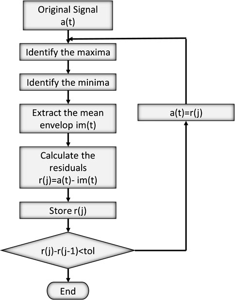
FIGURE 2. Flow chart of the EMD process.

The IMF modes represent smooth oscillatory time series instead of a simple harmonic function with a constant amplitude and frequency. Each mode can have different frequencies and amplitudes, and they can also have a single frequency with varying amplitudes, and some modes can have a harmonic response. The first step consisted of finding the IMF modes for the four signals (three accelerations and one deformation); then, the IMF was grouped into modes defining the rigid body motion and the vibration motion modes. The next step consisted of determining the relationship between the amplitudes of the acceleration and deformation amplitudes. This function was built only with the modes describing the rigid body motion.

All the strain gauge signals have a similar waveform, and the variations depend on the gauge’s position at the track.

The similarity among the data suggested that a single strain gauge could determine the deformation shape on the track. The following section showed the modes of the signals when the strain signal had high values. The data corresponds to the instant when the railcar is near the strain gauge.

Empirical mode decomposition results

Since the strain gauges were located in fixed positions, the strain measurement was significant when the railcar ran over them. Therefore, the correlation between the accelerometer and the strain gauge data could be valid at the data intervals before and after the maximum peak (equivalent to the sleeper’s spam). If there were a defect on the track away from the measuring device, the acceleration would have recorded a high peak at a different position; therefore, the strain gauge would never register that dynamic condition. Figure 3 presents the non-periodic and periodic modes for the strain gauge. The non-periodic modes are the first three Intrinsic Modes (IM), whereas the periodic modes are the remaining IM.

FIGURE 3

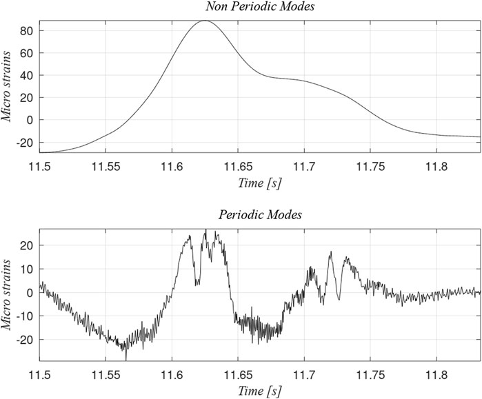
FIGURE 3. Comparison of the non-periodic and periodic intrinsic modes for the strain measured at the experimental rig.

Transfer function

The time series obtained during measurements are, in nature, non-periodic. Therefore, the transfer function cannot be obtained directly (De Santiago & San Andrés, 2007). Thus, both signals were decomposed into modes using the Empirical Mode Decomposition. Since the number of modes and the frequencies associated with each mode was different between the two signals, the assumption was that:

$\overline{f}=\left[H\right]{\overline{a}}^T(3)$

Where $\overline{f}$ is the deformation data, and its dimension depends on the number of points registered during the strain measurements. In this case, the sleeper-to-sleeper time was 1.25 s. All the strain gauges produced similar data, and the “Strain gauge 2” recorded the deformations caused by accelerations in the three directions. $\overline{a}$ is the acceleration data, and it is formed with RMS values of the non-periodic modes, and $\left[H\right]$ is the function transfer matrix. In this case, the dimensions of $\overline{f}$ is 1,000 × 1 and for $\overline{a}$ is 1 × 9.

The modes that best defined the transfer function were determined by comparing the signals. Each mode had one or more characteristic frequencies, and its amplitude varied with time; therefore, a spectrogram (time-frequency map) showed the frequency and time interval for the highest peak. Then, the transfer function was built with those modes that had similarities in frequency and time intervals (spectrograms). The first three modes correspond to the rigid body motion, which also caused the highest loads. These modes were the basis for defining the transfer function. Table 2 shows the frequency for the highest peak for each signal and each mode.

TABLE 2

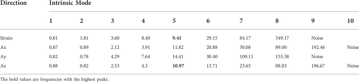
TABLE 2. Dominant frequencies for each periodic mode (Hz).

Interestingly, similar frequencies appear in the first three modes and mode 5. The highlighted frequencies at mode five were closed to the wheel’s rotation frequency. The difference among the frequencies from mode five could be caused by the friction or the wheel’s slip.

Figure 4 compares the spectrograms (time-frequency maps) of the sum of modes 1, 2, 3 (rigid body motion modes) and a comparison of mode 5 (wheels velocity); the spectrograms corresponded to the strain gauge identified as “Strain gauge 2” and the acceleration in the vertical direction. The comparison was made with all directions, but only the longitudinal direction was included. Not only are the frequencies similar, but the time intervals are equivalent in both maps. In this case, the sleeper-to-sleeper time was 1.25 s.

FIGURE 4

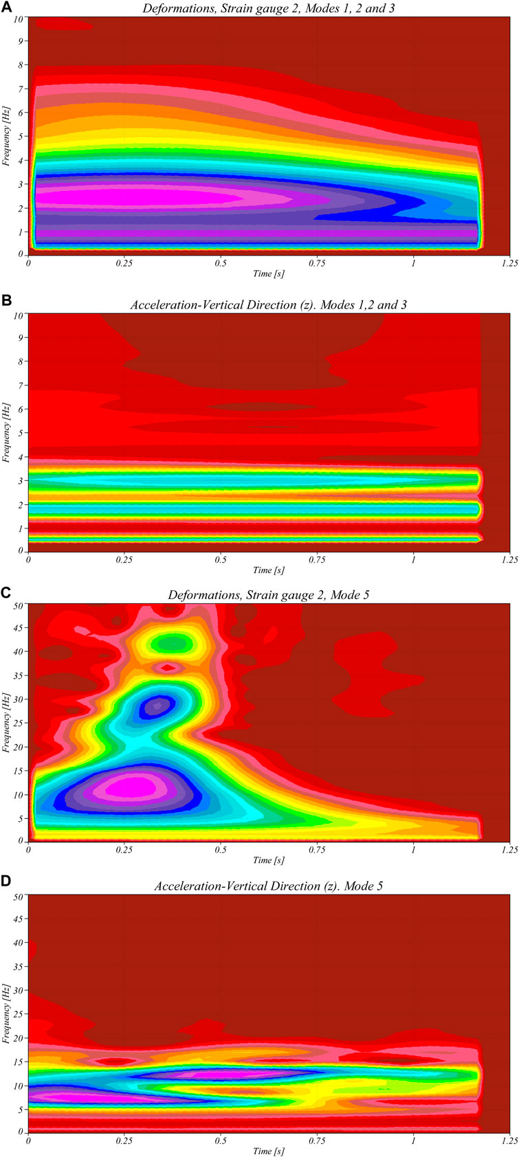
FIGURE 4. (Continued).

After analyzing the similarities between the signals, it was decided to build the transfer function only with the first three modes which corresponded to the rigid body motion. The fifth mode reflects the effect of the wheel’s angular speed, and its contribution to the overall amplitude is minimum. Besides this contribution, the wheel effect is related to other failure conditions that will be analyzed in future works.

Since $\left[H\right]$ is rectangular, it is necessary to find the pseudoinverse, and the only solution that avoids singularities is the Singular Value Decomposition (SVD) (Vega & Clainche, 2021). This procedure calculates the pseudoinverse of the matrix that relates the deformation data to the acceleration data. A simplified version of this procedure is:

$\left[H\right]=\overline{f}{\left[M\right]}^T(4)$

Where $\overline{f}$ contains the strain gauge data.

$\left[M\right]=\left[V\right]\left[S\right]\left[U\right](5)$

$\left[V\right]$ is a matrix with the eigenvectors of $\left[B\right]$, and $\left[B\right]$ is determined from the acceleration data as:

$\left[B\right]={\overline{a}}^T\overline{a}(6)$

Where $\overline{a}$ is a 1 × 9 horizontal vector

$\overline{a}=\left[\begin{array}{ccc}{a}_x& a_y& a_z\end{array}\right](7)$

And

$\begin{array}{c}{a}_x=\left[\begin{array}{ccc}\left|a_{x1}\right|& \left|a_{x2}\right|& \left|a_{x3}\right|\end{array}\right]\\ a_y=\left[\begin{array}{ccc}\left|a_{y1}\right|& \left|a_{y2}\right|& \left|a_{y3}\right|\end{array}\right]\\ a_z=\left[\begin{array}{ccc}\left|a_{z1}\right|& \left|a_{z2}\right|& \left|a_{k3}\right|\end{array}\right]\end{array}(8)$

Thus, the vector $\overline{a}$ contains the amplitude of the first three modes in each motion direction. $a_{ki}$ corresponds to modes 1, 2, and 3 for each direction $k$ For this case, the dimension of the vector $a$ is nine. This condition ensures that the measurements along the trajectory on the track include all the dynamic behavior’s contributions. The dimension of B is 9 × 9.

Following the SVD method, $\left[S\right]$ is a diagonal matrix containing the eigenvalues of $\left[B\right]$ (Eq. 6), and

$\left[V\right]=eig\left(\left[B\right]\right)=\left[\begin{array}{cc}{v}_1\dots & v_n\end{array}\right](9)$

And the elements of $\left[U\right]$ are:

$u_i=\frac{{\overline{a}}^T{v}_i}{s_{ii}}(10)$

and $s_{ii}$ are the elements of $\left[S\right]$

In this case $\left[V\right]$ is a 9 × 9 matrix, $\left[S\right]$ is a 9 × 9 matrix, and $\left[U\right]$ is a 9 × 1 matrix. Thus, $\left[M\right]$ is a 9 × 1 vector.

Once the matrix $\left[M\right]$ is determined, the calculation of the transfer function $\left[H\right]$ is straight-forward (Eq. (4))

Figure 5 describes the flow chart for the construction of the transfer function H.

FIGURE 5

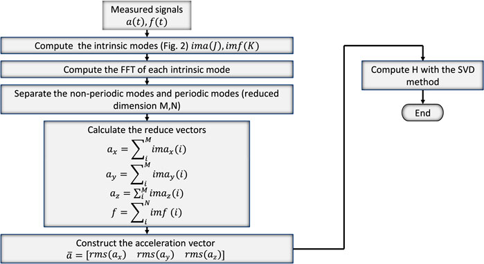
FIGURE 5. Flow chart for computing the transfer function H.

The application of this method to the data presented in previous sections produces a graphical matrix (Figure 6). This figure represents a contour plot of the matrix values, indicating the maxima’s location. The values correspond to matrix H coefficients. In this case, there were three non-periodic modes (modes 1,2, and 3); thus, the dimension of $\overline{a}$ is nine, and the dimension of $\overline{f}$ is the length of the intrinsic mode vector. This graph identifies each accelerometer’s relative contribution, and it is noticeable that the longitudinal acceleration has a higher effect.

FIGURE 6

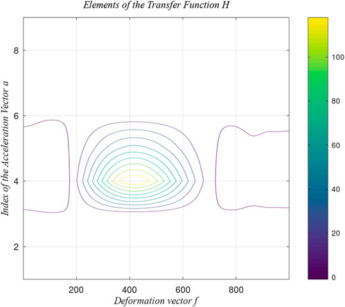
FIGURE 6. Contour map of the transfer matrix elements.

The matrix H is considered a signature or pattern of the local behavior along the track. This matrix is used as a shape basis for predicting the track deformation in the interaction wheel-track. Figure 7 shows the basis for predicting this deformation which is similar to the transfer function described by Esveld (Esveld, 2014), (Esveld et al., 1988). Esveld considered that the function is symmetric with respect to the application of the load, whereas, in this work, it was found that the shape is not symmetric due to the friction forces. The procedure is as follows:

− The accelerometers register the vibrations during the railcar traveling in the three directions (x, y, and z).

− The railcar’s speed determines the relationship between the time vector and the position vector. It is recorded during the railcar trip.

− The acceleration data is segmented in time intervals equivalent to the track’s deformation zone. (Figure 7). The data represent time windows with the length of the sleeper’s span; the time length may vary according to the railcar’s speed.

− For each acceleration vector ${\overline{a}}_m$, an equivalent RMS value determines the individual contribution to the track deformations $f_e$.

− Since the only measurements are the railcar accelerations, the estimated deformations are determined by applying the transfer function H (Eq. 3) to the acceleration measurements recorded in the Subway:

$\overline{f_e}=\left[H\right]{\overline{a}}_m$

− The full track deformation results from the superposition of each segmented vector along with the total data.

FIGURE 7

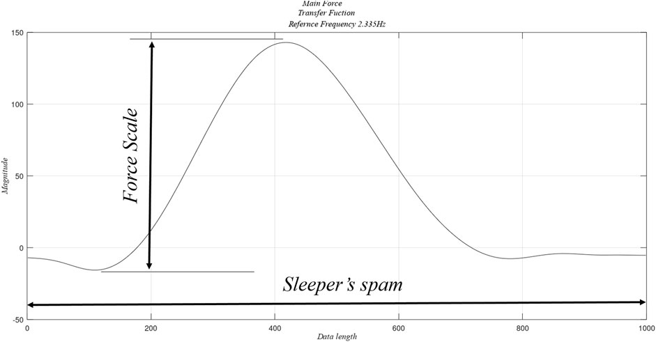
FIGURE 7. Base function for the deformation vector $\overline{\mathit{f}}$.

The transfer function considered the effect of the orthogonal vibration measurements (x,y, and z); the input function was the RMS acceleration amplitude estimated during a specific time interval. The railcar speed determines the time interval, and it is equivalent to the length of the rail’s deformed distance (the sleeper’s separation).

The transfer function can be applied to any acceleration measurements without measuring the track deformations. The following section describes the application of the transfer function for identifying a severe failure in a subway system.

Case study

This section presents the application of the transfer function for identifying the health condition of a substructure in a subway system. This study was the outcome of analyzing a failure that appeared in one of the structure inspections. The substructure was part of an elevated track that presented severe damage and caused a dramatic accident. Before the accident, the monitoring system only recorded vibration signals from a set of accelerometers mounted on the train, and the acceleration data complemented the regular maintenance procedure. Unfortunately, the acceleration data was dispersing, and it was not easy to correlate it with the actual dynamic loading on the substructure.

After a routine inspection, it was detected that the substructure of an elevated section of the track presented premature cracks. It was assumed that the crack was due to an earthquake. Therefore, it was decided to measure the dynamic effect of the train on the track. The health monitoring system consisted of accelerometers mounted on the train and the analysis algorithm. Measuring the track deformations was too expensive, and it required very complicated data acquisition equipment. Thus, the monitoring system relay on the acceleration measurements. The accelerometers were mounted underneath a bogie of one railcar (Figure 8). The train ran continuously, and in this paper, we present three runs recorded on different dates. The data corresponds to the train traveling along track B (Figure 9).

FIGURE 8

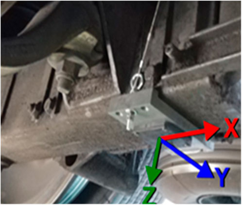
FIGURE 8. Sensor’s location in the bogie.

FIGURE 9

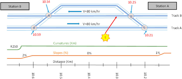
FIGURE 9. Track diagram in the area where the failure occurred (Point E).

The cracks on the substructure were located at the bridge near one of the subway stations. It was marked (Point E) on a track diagram described in Figure 9. The visual inspection identified that the sleepers were hanging (soft support), and the ballast had a different damping coefficient. It was estimated that 1 million railcars passed over the structure at the inspection time. This information confirmed that the failure was due to low cycle fatigue.

The first analysis developed the acceleration data’s spectrograms (time-frequency maps) using a similar procedure (Cho & Park, 2021). The spectrograms were produced with the Continuous Wavelet Transform and the Morlet function as the mother wavelet.

The data were recorded during the whole trajectory; the analysis was limited to the track section between the adjacent stations of the damaged area (Stations A and B in Figure 9). It is essential to point out that the section has only four clear external excitations, the switch tracks located at points A, B, C, and D.

For each run, the accelerations in the vertical direction (z), lateral direction (y), and motion direction 10 (×) were recorded with three MEM’s accelerometers. The gyroscopes’ data were not considered because the transfer function depends only on the accelerations. In this paper, only the results for one run are included.

The train’s speed is very similar in the three runs. Figure 10 shows the velocity profile when the train runs from Station A to Station B. The average speed was 12 m/s, and although there is a slight change in the average speed, the increment in the dynamic load is hardly observed in the acceleration data.

FIGURE 10

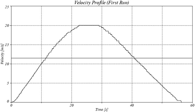
FIGURE 10. Velocity profile for the first run.

Figure 11 shows the spectrogram of the acceleration in the vertical direction. This figure contains the most significant dynamic load. The dominant frequencies are 5 Hz, 65 Hz, and 100 Hz. The 5 Hz frequency corresponds to the wheel’s rotation speed, and the other two are some of the train’s natural frequencies. The first and second runs show the highest peaks at 15 s and 65 Hz, whereas in the third run, the highest peak is at 35 s and 100 Hz.

FIGURE 11

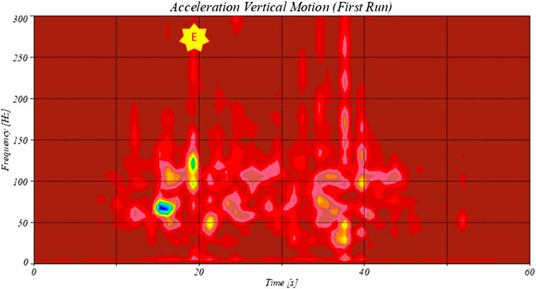
FIGURE 11. Spectrogram of the acceleration in the vertical direction (z). First run.

For a monitoring process, these variations on the acceleration spectrograms complicate the definition of failure criteria (Jauregui-Correa & Lozano-Guzmán, 2020). A more reliable analysis included the application of the transfer function (Eq. 3)

Application of the transfer function

The transfer function transforms the dynamic loads (accelerations) into the tracks deformations. This transformation combines the effects of the three acceleration components into an equivalent track deformation. This deformation transmitted forces to the substructure through the sleepers and ballast.

The deformation data (Figure 3) was scaled using the train’s weight. The scale factor was determined by dividing the railcar weight into the number of wheels. Figure 12 shows the estimated deformation for the first runs. The pattern reflects the dynamic load changes and the location of the highest amplitudes.

FIGURE 12

FIGURE 12. Estimated track deformations between stations A and B

Figures 13–15 show the spectrogram of the estimated track deformations. The three diagrams show similar patterns, with three dominating frequencies, one at low frequency, which corresponds to the weight, and the other two are passing sleepers frequency (15 Hz) and its harmonics (30 Hz). The highest amplitudes correspond to the points where the substructure had the highest fatigue loads.

FIGURE 13

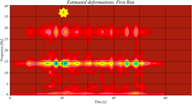
FIGURE 13. Spectrogram of the estimated deformations (First run).

FIGURE 14

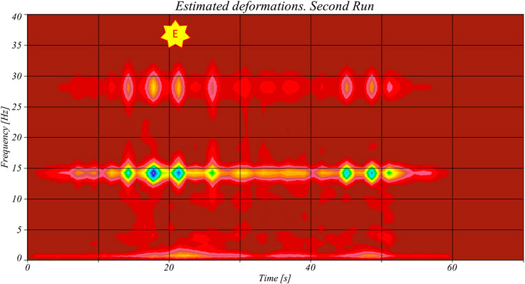
FIGURE 14. Spectrogram of the estimated deformations (Second run).

FIGURE 15

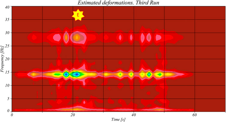
FIGURE 15. Spectrogram of the estimated deformation (Third run).

The health monitoring system measures the accelerations with accelerometers mounted underneath the bogie, estimating the equivalent dynamic force on the track and substructure and identifying the highest deformations. The estimated deformation is obtained with the transfer function developed in an experimental rig, and it was determined with the Empirical Mode Decomposition Method.

These figures show the frequency variations as the train moves from station A to station B. The first and third data runs show the highest peak at point E and the passing sleepers frequency (15 Hz). The second run shows the highest peat at the switchgear (point A in Figure 9). The data from the three runs show a high peak at point E at the lowest frequency. Comparing Figures 13–15 with the spectrogram of the acceleration data (Figure 11), it is clear that the effect of the soft sleeper (point E) is less significant in the acceleration data than in the deformation spectrograms. Therefore, the acceleration data is less confident in predicting the dynamic effect of a passing train, and it could mislead the identification of failures in the track or the substructure.

Stations A and B track is almost straight, with two rail switchgear. In this case study, the measurements were recorded on track B. There was two switchgear located at points D and A (according to the direction of motion). The switchgear creates impacts that are always present in every measurement. The switchgear at point D produces three peaks at 15, 16, and 18 s (Figure 13). The switchgear A makes another three peaks at 48, 52, and 58 s. If the track were healthy, the only significant peaks were the switchgear, but in this case, there is another peak located at point E. Before analyzing the data, it is essential to identify the installed elements that produce higher vibrations, such as switchgear or instruments, since the spectrograms will display those impacts as high peaks. Peaks that appear elsewhere are related to defects or failures in the track or substructure, and these points must be inspected regularly.

After a visual inspection of the tracks, it was found that point E corresponded to a soft sleeper. It was also found that the ballast had a low damping property than the ballast specified in the design. The increment in the dynamic load and the low damping coefficient incremented the fatigue load that started the crack in the substructure.

Conclusion

Monitoring is focused on finding faults and predicting degradation on the tracks. The method presented in this paper transforms train acceleration measurements into track loads. With this approach, the train’s motion is utilized to identify variations in the track’s deformations without installing instruments. It was found that this method was able to locate the dynamic impacts produced by well-located track elements, such as switchgear or instrumentations, and to identify vibration sources that have no relation to any specific part. Before analyzing the data, it is essential to identify the installed factors that produce higher vibrations, such as switchgear or instruments, since the spectrograms will display those impacts as high peaks. Peaks that appear elsewhere are related to defects or failures in the track or substructure, and these points must be inspected regularly.

The transfer function was characterized as a linear transformation, and the transformation base was the matrix H. This matrix worked as a filter and separated the dynamic loads associated with the train’s translation from the vibration loads related to the wheel’s rotation or other vibration sources. The EMD was the method that allowed the separation of the non-periodic and periodic elements that formed the original data.

This method allowed the identification of failures in a Subway system, and it was more accessible to local crack initiations on the substructure. Traditional methods cannot identify large deformations because they measure track deformations without the actual train’s load.

The transfer function transformed the acceleration data into track deformations. The deformation pattern obtained experimentally is similar to a theoretical model, and the waveform depends on the sleepers’ stiffness. This fact confirmed its applicability to field data. Although there is a need for more experimental data, the transfer function can be applied to acceleration data recorded from subways systems with metal wheels. A new test rig is under construction to validate the results presented in this paper.

Future work will define a predicting program by storing the acceleration data from trains running on the track, transforming the acceleration data into track deformations, and analyzing the evolution of the higher peaks as a function of train runs.

Data availability statement

The raw data supporting the conclusion of this article will be made available by the authors, without undue reservation.

Author contributions

All authors listed have made a substantial, direct, and intellectual contribution to the work and approved it for publication.

Conflict of interest

The authors declare that the research was conducted in the absence of any commercial or financial relationships that could be construed as a potential conflict of interest.

Publisher’s note

All claims expressed in this article are solely those of the authors and do not necessarily represent those of their affiliated organizations, or those of the publisher, the editors and the reviewers. Any product that may be evaluated in this article, or claim that may be made by its manufacturer, is not guaranteed or endorsed by the publisher.

References

Akutagawa, K., and Wakao, Y. (2018). “Stabilization of Vehicle Dynamics by Tire Digital Control - tire disturbance control algorithm for electric motor drive system,” in 31st International Electric Vehicle Symposium and Exhibition, EVS 2018 and International Electric Vehicle Technology Conference 2018, EVTeC 2018, 1–10.

Google Scholar

Cantero, D., McGetrick, P., Kim, C. W., and OBrien, E. (2019). Experimental monitoring of bridge frequency evolution during the passage of vehicles with different suspension properties. Eng. Struct. 187, 209–219. doi:10.1016/j.engstruct.2019.02.065

CrossRef Full Text | Google Scholar

Chang, C., Ling, L., Han, Z., Wang, K., and Zhai, W. (2019). High-speed train-track-bridge dynamic interaction considering wheel-rail contact nonlinearity due to wheel hollow wear. Shock Vib. 2019, 1–18. doi:10.1155/2019/5874678

CrossRef Full Text | Google Scholar

Chen, Z., and Fang, H. (2019). An alternative solution of train-track dynamic interaction. Shock Vib. 2019, 1–14. doi:10.1155/2019/1859261

CrossRef Full Text | Google Scholar

Cheng, J., Yu, D., and Yang, Y. (2008). A fault diagnosis approach for gears based on IMF AR model and SVM. EURASIP J. Adv. Signal Process. 2008, 647135. doi:10.1155/2008/647135

CrossRef Full Text | Google Scholar

Cho, H., and Park, J. (2021). Study of rail squat characteristics through analysis of train axle box Acceleration frequency. Appl. Sci. Switz. 7022, 7022. doi:10.3390/app11157022

CrossRef Full Text | Google Scholar

Ciotlaus, M., Kollo, G., Marusceac, V., and Orban, Z. (2019). Rail-wheel interaction and its influence on rail and wheels wear. Procedia Manuf. 32, 895–900. doi:10.1016/j.promfg.2019.02.300

CrossRef Full Text | Google Scholar

Daniel, Ľ., and Kortiš, J. (2017). The comparison of different approaches to model vehicle-bridge interaction. Procedia Eng. 190, 504–509. doi:10.1016/j.proeng.2017.05.370

CrossRef Full Text | Google Scholar

Davis, N. T., and Sanayei, M. (2020). Foundation identification using dynamic strain and acceleration measurements. Eng. Struct. 208, 109811. doi:10.1016/j.engstruct.2019.109811

CrossRef Full Text | Google Scholar

De Santiago, O., and San Andrés, L. (2007). Field methods for identification of bearng support parameters—Part I: Identification from transient rotor dynamic response due to impacts. J. Eng. Gas Turbines Power 129 (1), 205–212. doi:10.1115/1.2227033

CrossRef Full Text | Google Scholar

Dumitriu, M., and Gheţi, M. A. (2019). Cross-correlation analysis of the vertical accelerations of railway vehicle bogie. Procedia Manuf. 32, 114–120. doi:10.1016/j.promfg.2019.02.191

CrossRef Full Text | Google Scholar

Entezami, A., and Shariatmadar, H. (2019). Structural health monitoring by a new hybrid feature extraction and dynamic time warping methods under ambient vibration and non-stationary signals. Meas. (. Mahwah. N. J). 134, 548–568. doi:10.1016/j.measurement.2018.10.095

CrossRef Full Text | Google Scholar

Esen, İ. (2011). Dynamic response of a beam due to an accelerating moving mass using moving finite element approximation. Math. Comput. Appl. 16 (1), 171–182. doi:10.3390/mca16010171

CrossRef Full Text | Google Scholar

Esveld, C., Jourdain, A., Kaess, G., and Shenton, M. J. (1988). Historic data on track geometry in relation to maintenance. Rail Eng. Int. Ed. 2, 16–19.

Google Scholar

Esveld, C. (2014). Modern railway track (digital). MRT-Productions, Delft University of Technology.

Google Scholar

Fermér, M., and Nielsen, J. C. O. (1995). Vertical interaction between train and track with soft and stiff railpads—Full-scale experiments and theory. Proc. Institution Mech. Eng. Part F J. Rail Rapid Transit 209 (1), 39–47. doi:10.1243/PIME_PROC_1995_209_253_02

CrossRef Full Text | Google Scholar

Hoang, T., Fu, Y., Mechitov, K., Gómez-Sánchez, F., Kim, J. R., Zhang, D., et al. (2020). Autonomous end-to-end wireless monitoring system for railroad bridges. Adv. Bridge Eng. 7, 17–27. doi:10.1186/s43251-020-00014-7

CrossRef Full Text | Google Scholar

Jaschinski, A., Chollet, H., Iwnicki, S., Wickens, A., and Von Würzen, J. (1999). The application of roller rigs to railway vehicle dynamics. Veh. Syst. Dyn. 31 (5–6), 345–392. doi:10.1076/vesd.31.5.345.8360

CrossRef Full Text | Google Scholar

Jauregui-Correa, J. C., and Lozano-Guzmán, A. (2020). Mechanical vibrations and condition monitoring. Netherlands: Elsevier.

Google Scholar

Koç, M. A., Esen, İ., Eroglu, M., and Cay, Y. (2021). A new numerical method for analysing the interaction of a bridge structure and travelling cars due to multiple high-speed trains. Int. J. Heavy Veh. Syst. 28 (1), 79. doi:10.1504/ijhvs.2021.114415

CrossRef Full Text | Google Scholar

Koc, M. A., Esen, I., Eroglu, M., Cay, Y., and Cerlek, O. (2018). Dynamic analysis of flexible structures under the influence of moving multiple vehicles. El-Cezeri J. Sci. Eng. 5 (1), 176–181. doi:10.31202/ecjse.354769

CrossRef Full Text | Google Scholar

Koç, M. A., and Esen, İ. (2017). Modelling and analysis of vehicle-structure-road coupled interaction considering structural flexibility , vehicle parameters and road roughness. J. Mech. Sci. Technol. 31 (5), 2057–2074. doi:10.1007/s12206-017-0403-y

CrossRef Full Text | Google Scholar

Liu, Y., Sun, X., Hock, J., and Pang, L. (2020). A YOLOv3-based deep learning application research for condition monitoring of rail thermite welded joints. IVSP ’20 Proc. 2020 2nd Int. Conf. Image, Video Signal Process., 33–35.

CrossRef Full Text | Google Scholar

Malekjafarian, A., and OBrien, E. J. (2017). On the use of a passing vehicle for the estimation of bridge mode shapes. J. Sound Vib. 397, 77–91. doi:10.1016/j.jsv.2017.02.051

CrossRef Full Text | Google Scholar

Malekjafarian, A., OBrien, E., Quirke, P., and Bowe, C. (2019). Railway track monitoring using train measurements: An experimental case study. Appl. Sci. Switz. 9 (22), 4859. doi:10.3390/app9224859

CrossRef Full Text | Google Scholar

Mizrak, C., and Esen, I. (2015). Determining effects of wagon mass and vehicle velocity on vertical vibrations of a rail vehicle moving with a constant acceleration on a bridge using experimental and numerical methods. Shock Vib., 1–15. doi:10.1155/2015/183450

CrossRef Full Text | Google Scholar

Molodova, M., Oregui, M., Núñez, A., Li, Z., and Dollevoet, R. (2016). Health condition monitoring of insulated joints based on axle box acceleration measurements. Eng. Struct. 123, 225–235. doi:10.1016/j.engstruct.2016.05.018

CrossRef Full Text | Google Scholar

Naeimi, M., Li, Z., Dollevoet, R., and Law, A. S. (2014). Scaling Strategy a New Exp. Rig Wheel-Rail Contact 8 (12).

Ngamkhanong, C., Kaewunruen, S., and Alfonso-Costa, B. (2018). State-of-the-Art review of railway track resilience monitoring. Infrastructures (Basel). 1, 3. –18. doi:10.3390/infrastructures3010003

CrossRef Full Text | Google Scholar

Pehlivan, F., Mizrak, C., and Esen, I. (2018). Modeling and validation of 2-DOF rail vehicle model based on electro – mechanical analogy theory using theoretical and experimental methods. Eng. Technol. Appl. Sci. Res. 8 (6), 3603–3608. doi:10.48084/etasr.2420

CrossRef Full Text | Google Scholar

Quirke, P., Cantero, D., Obrien, E. J., and Bowe, C. (2017). Drive-by detection of railway track stiffness variation using in-service vehicles. Proc. Institution Mech. Eng. Part F J. Rail Rapid Transit 231 (4), 498–514. doi:10.1177/0954409716634752

CrossRef Full Text | Google Scholar

Romero Navarrete, J. A., and Otremba, F. (2020). A testing facility to assess railway car infrastructure damage. A conceptual design. Int. J. TDI. 4 (2), 142–151. doi:10.2495/TDI-V4-N2-142-151

CrossRef Full Text | Google Scholar

Shi, L., Zhu, Y., Zhang, Y., and Su, Z. (2021). Fault diagnosis of signal equipment on the lanzhou-xinjiang high-speed railway using machine learning for natural language processing. Complexity 2021, 1–13. doi:10.1155/2021/9126745

CrossRef Full Text | Google Scholar

Smith, R. A. (2005). Railway fatigue failures : An overview of a long standing problem. Materwiss. Werksttech. 36 (11), 697–705. doi:10.1002/mawe.200500939

CrossRef Full Text | Google Scholar

Thompson, D. (2014). “Railway noise and vibration : The use of appropriate models to solve practical problems,” in The 21 St International Congress on Sound and Vibration, 13–17.

Google Scholar

Turner, C., Tiwari, A., Starr, A., and Blacktop, K. (2016). A review of key planning and scheduling in the rail industry in Europe and UK. Proc. Institution Mech. Eng. Part F J. Rail Rapid Transit 230 (3), 984–998. doi:10.1177/0954409714565654

CrossRef Full Text | Google Scholar

Usman, K., Burrow, M., and Ghataora, G. (2015). Railway track subgrade failure mechanisms using a fault chart approach. Procedia Eng. 125, 547–555. doi:10.1016/j.proeng.2015.11.060

CrossRef Full Text | Google Scholar

Vega, J. M., and Clainche, S. Le. (2021). General introduction and scope of the book. In J. M. Vega, and S. Le Clainche (Eds.), Higher order dynamic mode decomposition and its applications (pp. 1–28). Elsevier B, Netherlands.V. doi:10.1016/B978-0-12-819743-1.00008-2

CrossRef Full Text | Google Scholar

Weston, P., Roberts, C., Yeo, G., and Stewart, E. (2015). Perspectives on railway track geometry condition monitoring from in-service railway vehicles. Veh. Syst. Dyn. 53 (7), 1063–1091. doi:10.1080/00423114.2015.1034730

CrossRef Full Text | Google Scholar

Zhai, W., and Wang, K. (2010). Lateral hunting stability of railway vehicles running on elastic track structures. J. Comput. Nonlinear Dyn. 5 (4), 1–9. doi:10.1115/1.4001908

CrossRef Full Text | Google Scholar