Prediction of Compressor Blade Erosion Experiments in a Cascade Based on Flat Plate Specimen

1 Introduction

Jet engine fans and high-pressure compressors suffer significantly from solid particle erosion (Brandes et al., 2021). Their particular erosive environment is characterized by high momentum particle impacts on thin airfoils resulting in changes in airfoil shape. Some service experience is published for selected engines (Sallee, 1978). In general, “pitting and cutting back of the leading edges and thinning of the trailing edges” (Grant and Tabakoff, 1975) results in a shortening of the chord length of axial compressor blades. This is accompanied by a general increase in surface roughness (Balan and Tabakoff, 1984).

Generally, solid particle erosion involves the transport of the particles in the fluid flow (Ghenaiet, 2012; Hussein and Tabakoff, 1974), particle wall interaction Bons et al. (2017), particle fracture (Hadavi et al., 2016; Sommerfeld et al., 2021), and material loss. The representation of these processes requires complex numerical models that correctly reproduce the transport of the particles in a compressible, turbulent, and unsteady flow typical to turbojet engines (e.g., Kopper et al. (2019)). This allows the kinematics of individual particle impacts on the surface elements of a discretized structure to be calculated (see Figure 1). Considering particle breakage and material loss in the blades caused by single-particle impacts imposes significant computational efforts and still requires semi-empirical correlations like the Johnson–Cook model for the high-speed strain behavior of ductile blade materials and the Johnson–Holmquist-II model for brittle particle materials (Du et al., 2021). The high resolution of the numerical approach is achieved at the cost of high computational resources. The computational representation of the erosion-related wear on a blade during its operational life thus entails unmanageable computation times.

FIGURE 1

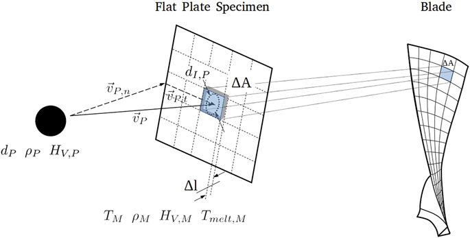
FIGURE 1. Kinematics of an individual particle impact transitioned from a flat plate specimen to a surface element on a blade.

With an alternative approach, the cumulative effect of a multitude of particle impacts on a single surface element during a given time step Δt is taken into account. Therefore, mean values of the erosive parameters have to be derived for each time step. The resulting loss of material assigned to the surface element ΔA then is derived using an empirical parameter, the so-called erosion rate e.

Sandblast facilities providing a small jet of particle-laden air impacting stationary flat plate specimens are used to experimentally characterize the erosion rate $e=\frac{\mathrm{\Delta }{m}_M}{m_P}$ for a given combination of particle type and specimen material. An overview of such experiments is given in Hamed et al. (2006). Careful correction based on nondimensional groups is needed to make such test results generally applicable to other cases (Hufnagel et al., 2017; Hufnagel et al., 2018). The erosive change of shape of a compressor blade can be predicted by assuming that the erosion of discrete elements of the blade surface can be related to these flat plate experiments (Marx, 2013; Schrade, 2015; Schrade et al., 2015). Herein, the erosion rate e functions as an integral parameter. It gives the advantage to cover details of the material loss processes such as the roughening of the surface (Mora et al., 2019) and gradual changes of the surface shape due to repeated particle impacts. This approach allows a good approximation to the experimentally determined erosion-induced shape change under the use of little computational power, which enables the simulation of the change in shape of a blade during its entire period of operation.

Based on a well-known particle transport, two main questions need to be answered to apply the introduced approach. First, the application limits of the erosion rate e as an integral parameter have to be clarified. Thus, the erosion rate e can be adapted to numerical computations of the erosive change of shape on discretized surfaces of blades and vanes. Second, the spatial and temporal discretization including the representation of the eroded geometry need elaboration. The prediction of the worn compressor blade geometry generated in a linear erosion cascade facilitates this discussion.

2 Particle Impact on a Surface Element

The application of the erosion rate e derived from flat plate experiments to the numerical prediction of the erosive change of shape of arbitrary geometries such as compressor blades and vanes imposes limits on the spatial and time resolution. These limits are elaborated by an extension of the dimensional analysis presented in Hufnagel et al. (2017) to particles impacting the flat surface of a specimen which is discretized into surface elements ΔA as it is shown in Figure 1. It comprises particles of diameter d_P, density ρ_P, and hardness H_V,P impacting with the velocity v_P. The area affected by the particle impact is characterized by its diameter d_I,P. The material of the surface element is characterized by its density ρ_M and hardness H_V,M, melting temperature T_melt,M, and actual temperature T_M. It is assumed that the impacts happen at a frequency f during a time step Δt. As a result of the repeated impacts during the time step, the surface of the element ΔA steps back by an increment Δl.

A nondimensional representation of the erosion rate is found using the Buckingham Π theorem with the dimensional matrix depicted in Table 1. It is documented in Eq. 1.

$\frac{\mathrm{\Delta }A}{\mathrm{\Delta }{l}^2}=F\left(f\mathrm{\Delta }t,\frac{d_P}{\mathrm{\Delta }l},\frac{d_P}{d_{I,P}},\frac{v_{P,n}}{v_{P,t}},\frac{v_{P,n}^2{\rho }_P}{H_{v,M}},\frac{v_{P,t}^2{\rho }_P}{H_{v,M}},\frac{{\rho }_M}{{\rho }_P},\frac{H_{v,P}}{H_{v,M}},\frac{T_M}{T_{\mathit{melt,M}}}\right).(1)$

TABLE 1

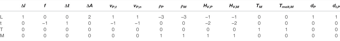
TABLE 1. Dimensional matrix repeated particle impact.

The last five nondimensional groups are already discussed in Hufnagel et al. (2017). The left-hand nondimensional group in Eq. 1 describes the surface step back relative to the surface element area. It is important to notice that the erosion rate e as a ratio of masses does not naturally relate to the surface step back. The density ratio of material and particles as well as the nondimensional groups $\frac{d_P}{\mathrm{\Delta }l}$ and Δtf are required to do so. According to Eq. 2, application of the erosion rate e implicitly requires a given spatial and time resolution.

$e=\frac{\mathrm{\Delta }A}{\mathrm{\Delta }{l}^2}\frac{{\rho }_M}{{\rho }_P}\frac{\mathrm{\Delta }{l}^3}{d_P^3}\frac{1}{\mathrm{\Delta }tf}=\frac{\mathrm{\Delta }A\mathrm{\Delta }l{\rho }_M}{d_P^3{\rho }_P\mathrm{\Delta }tf}=\frac{\mathrm{\Delta }{m}_M}{\frac{6}{\pi }{m}_P}.(2)$

Consequently, applying the erosion rate e derived from flat plate experiments to computations of high time resolution and highly discretized surfaces as shown in Figure 1 requires similarity of the first three nondimensional groups on the right-hand side of Eq. 1. The first nondimensional group Π₁ = f ⋅Δt is the number of impacts on the surface elements. With this in mind, the erosion rate e is interpreted as an integral result of a statistically relevant number of particle impacts on a flat plate surface element ΔA. The second nondimensional group ${\mathrm{\Pi }}_2=\frac{d_P}{\mathrm{\Delta }l}$ is a measure of the surface setback on which the experimentally obtained erosion rate is based on. Expansion of the third nondimensional group Π₃ by the nondimensional erosion rate $\frac{\mathrm{\Delta }A}{\mathrm{\Delta }{l}^2}$ and the second nondimensional group Π₂ leads to the derivative ${\acute{\mathrm{\Pi }}}_3$ which is documented in Eq. 3.

${\acute{\mathrm{\Pi }}}_3=\frac{d_P}{d_{I,P}}\frac{\mathrm{\Delta }l}{d_P}\sqrt{\frac{\mathrm{\Delta }A}{\mathrm{\Delta }{l}^2}}=\frac{\sqrt{\mathrm{\Delta }A}}{d_{I,P}}.(3)$

${\acute{\mathrm{\Pi }}}_3$ is a measure for the amount of surface elements ΔA which are affected by a single particle impact. The requirement to limit the effect of a single particle impact to one surface element ΔA leads to Eq. 4.

$\sqrt{\mathrm{\Delta }A}\ge d_P\frac{d_{I,P}}{d_P}.(4)$

${\acute{\mathrm{\Pi }}}_3$ becomes accessible by considering the energies of a plastic-elastic impact of a spherical particle on a flat surface (Bitter, 1963). The diameter of the impact area d_I,P increases with increasing particle excess velocity v_P − v_el beyond the maximum impact speed v_el of a purely elastic impact. The approximate solution for the plastic-elastic impact is given in Eq. 5 and Eq. 6. It represents the approximate solution with a negligible deviation.

$\frac{d_{I,P}}{d_P}={\left(\frac{8}{3}\frac{{\rho }_P}{y_M}{\left(v_P-v_{el}\right)}^2\right)}^{\frac{1}{4}},(5)$

$v_{el}=\frac{{\pi }^2}{2\cdot \sqrt{10}}{y}_M^{\frac{5}{2}}{\rho }_P^{-\frac{1}{2}}{\left[\frac{1-q_P^2}{E_P}+\frac{1-q_M^2}{E_M}\right]}^2.(6)$

Eq. 6 reveals that particle impact velocity v_P as well as the material values of the particles and the specimen such as the Poisson’s ratio (q_M, q_P), Young’s modulus (E_M, E_P), the material’s elastic load limit y_M, and the particle density ρ_P influence the spatial discretization. These three nondimensional parameters act as defining the spatial and time resolution of numerical simulations of solid particle erosion.

3 Spatial and Time Resolution

Limits for these three nondimensional parameters are derived for the erosion rates which emerge from the flat plate experiments described in Hufnagel et al. (2017) and Hufnagel et al. (2018). Arizona Road Dust A3 of a known particle diameter distribution is used in combination with the Ti-6Al-4V test specimen. The surface of the square, flat plate specimen is 50 mm in side length. For a Monte Carlo Simulation, a single, discrete square surface element of the size ΔA (see Figure 1) is considered. The diameter of the particles impacting this surface element is randomly selected while maintaining the known particle diameter distribution of Arizona Road Dust A3. 250 ⋅ 10⁶ particle impacts on the entire flat plate specimen are simulated. Consequently, the number of impacts on a single surface element drops as their number increases or their size ΔA decreases. Below a certain side length $\sqrt{\mathrm{\Delta }A}$, the diameter distribution of the particles impacting the surface element does not replicate the distribution of the test sand anymore. In this case, the ratio of material loss experienced by the surface element ΔA to the mass of particles, which impacted the surface element, does not match the erosion rate derived from flat plate experiments.

Hence, the goodness of fit of the size distribution of particles impacting the surface element with that of the Arizona Road Dust A3 provides a quantifiable measure to determine the number of necessary impacts on a surface element. The goodness of fit is tested based on the chi-square distribution (Montgomery et al., 2004). The test statistic is described in Eq. 7.

${\chi }^2=\sum _{i=1}^n\frac{{\left(f_{\mathit{observed}}\left(d_P\right)-f_{\mathit{Sand}}\left(d_P\right)\right)}^2}{f_{\mathit{Sand}}\left(d_P\right)},(7)$

${\chi }^2<{\chi }_{05,1}^2=3.841.(8)$

With a degree of freedom of 1 and an applied confidence limit of 95%, χ² holds a value of χ² = 3.841. The achieved goodness of fit and the confidence limit are documented in Figure 2. This, in turn, leads to a minimum of 488 impacts to replicate the particle size distribution of the test sand. This number is used as a lower limit for the first nondimensional group Π₁.

FIGURE 2

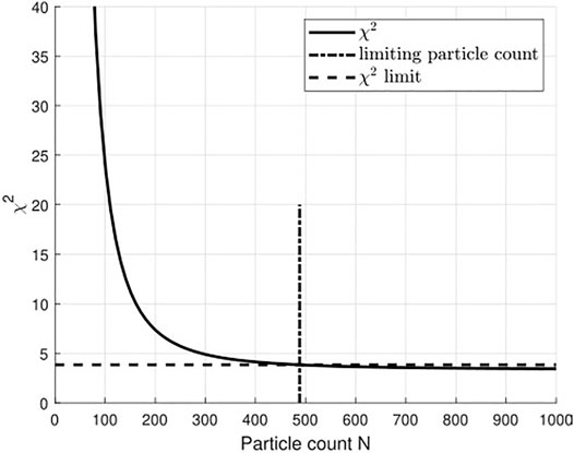
FIGURE 2. Goodness of fit for varying numbers of impacts.

A descriptive limit for the surface setback ${\mathrm{\Pi }}_2=\frac{d_P}{\mathrm{\Delta }l}$ is derived from the characteristics of the flat plate experiment. The effect of the shape change of the flat plate due to the evolving erosion crater is neglected, and all parameters are related to the uneroded flat plate surface. It limits the area-averaged regression to an order of magnitude smaller than the maximum particle diameter. This relation can be expressed by Eq. 9 and results in Δl_max < 0.025 mm for the given test sand.

${\mathrm{\Pi }}_{2,min.}=\frac{d_{P,max}}{\mathrm{\Delta }{l}_{max.}}>10.(9)$

The third nondimensional group Π₃ has been evaluated using the values documented in Table 2. The yield strength R_P0,2 given in Table 2 requires adjustment due to cold deformation hardening resulting from repeated particle impacts. For this purpose, a correction factor of 3.2 is applied according to Bitter (1963). This results in a yield strength of y_M = 2,656.0 N mm⁻². The third nondimensional group ${\mathrm{\Pi }}_3=\frac{d_{I,P}}{d_p}$ is shown in Figure 3 as a function of the yield strength for the approximate solution displayed in Eqs 5, 6. Evaluating this relationship leads to ${\mathrm{\Pi }}_3=\frac{d_{I,P}}{d_p}=0.658$.

TABLE 2

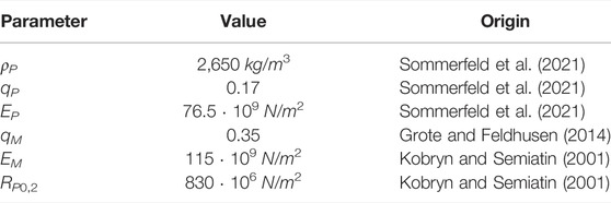
TABLE 2. Material parameters.

FIGURE 3

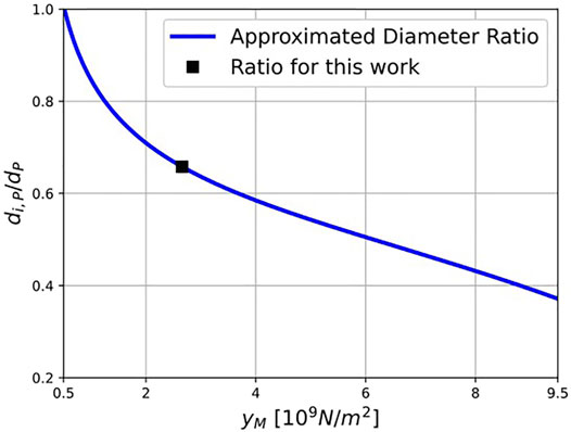
FIGURE 3. Ratio of impact diameter to particle diameter for plastic-elastic impact.

A sufficient accuracy is achieved if 99.73% of the particle impacts, representing a ± 3σ limit, only affect one surface element. The remaining rare impacts have a minuscule erosive effect on the surface elements since they are randomly spread across a large number of surface elements. 95.73% of particles of the used test dust are smaller than 0.230 mm. Requiring the impacts of 99,73% of the particles not affecting more than one surface element “and considering the value of Π₃” leads to a lower element size$\sqrt{\mathrm{\Delta }A}\le 0.15\mathrm{m}\mathrm{m}$ (see Eq. 4).

The requirement to limit the effect of one particle impact to one single finite volume $({\acute{\mathrm{\Pi }}}_3)$ defines the degree of spatial discretization of the surface for the particular case presented here. The time discretization is affected by the number of impacts required (Π₁) and the allowable surface setback (Π₂).

4 Local Surface Setback

The computation of the local surface setback due to erosion is based on Wong et al. (2012), Marx et al. (2014), Schrade et al. (2015), and Schrade (2015). Fulfilling the limits to discretization discussed in Section 3, it is assumed that the erosion rates derived from flat plate experiments are applicable throughout the complete erosive process. The particle transport to and from the surface is considered separately. As shown in Figure 1, the surface exposed to solid particle erosion is discretized into linear segments spanning flat surface elements between the surface grid points. Material loss due to solid particle erosion results in a three-dimensional change of the surface geometry. This is modeled by shifts of the flat surface elements which are consistent with the according loss in material volume. The required geometric parameters are shown in Figure 1.

In accordance with Libertowski et al. (2020), erosion is simulated by a multi-step procedure. Within a time step Δt, particles of mass m_P impact a surface element ΔA with velocity v_P at an impact angle ξ. The eroded volume ΔV is derived from the erosion rate e according to Eq. 10.

$\mathrm{\Delta }V=\mathrm{\Delta }ldadh=m_P\frac{e\left(\xi ,v_P\right)}{{\rho }_M}={\dot{m}}_P\frac{e\left(\xi ,v_P\right)}{{\rho }_M}\mathrm{\Delta }t.(10)$

Eq. 10 is applicable directly to discretized planar surfaces without the need for iteration. On a curved surface, solid particle erosion reduces the blade circumference and thus the base length da of the surface elements to db as shown in Figure 4. For a given eroded volume, the step back of the surface element Δl is corrected to $\acute{\mathrm{\Delta }l}$ which is defined in Eq. 11.

$dadh\mathrm{\Delta }l=\frac{da+db}{2}dh\acute{\mathrm{\Delta }l}.(11)$

FIGURE 4

FIGURE 4. Area correction for curved surfaces.

With both db and $\acute{\mathrm{\Delta }l}$ being unknown in Eq. 11, a four-step meshing approach is chosen to enable calculation on an eroded contour which is continuous and consistent with the computed eroded volumes of the individual surface elements. The starting point is the discretization of the surface fulfilling the requirements imposed by the nondimensional groups discussed in Section 3.

In the first step, the contour of the eroded surface is estimated such that Δl fulfills Eq. 9 and, hence, surely covers the step back of the surface elements expected for the time step (Figure 5A). The initial direction of the step backs is set perpendicular to the surface of the respective elements at the contact lines. This defines the taper of the volume elements and gives a relation $db=F(\acute{\mathrm{\Delta }l})$ which allows to solve Eq. 11 and to determine the step back $\acute{\mathrm{\Delta }l}$ specific to each surface element (Figure 5B). The resulting discontinuities at the element boundaries are eliminated by applying a central difference scheme, acquiring a smooth geometry (Figure 5C). The limitation of the simulation time steps and the high level of discretization of the blade surface results in a volumetric error per surface element ΔA which is negligible. New surface points are found on the piecewise linearized surface according to the requirements imposed by the nondimensional groups discussed in Section 2 (Figure 5D). Mesh morphing attempts have been discarded due to violation of the limits of spatial discretization which became visible in the resulting leading-edge geometries. Thereafter, the numerical flux at the end of the eroded contour is taken into account by applying the central difference scheme to the last eroded element and the first non-eroded element. This correction is cascaded into the eroded part of the contour until the calculated numerical flux vanishes.

FIGURE 5

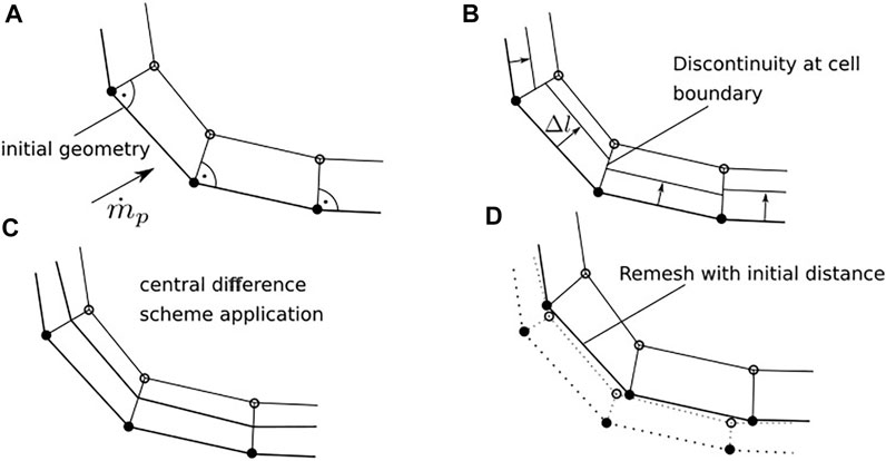
FIGURE 5. Remesh Procedure that captures the step back (A), has discontinuities at the cell boundaries (B), uses a central difference scheme for an continuous representation of the new geometry (C) and re-meshes the geometry with the initial distance (D).

5 Representation of the Eroded Surfaces

Determining the surface step back in accordance with Section 4 requires guessing the eroded surface in step a and determining it in step c as shown in Figure 5. The representation of this surface has to fulfill three main requirements:

1) Accurately reproduce the surface of new and eroded blades or vanes including the leading edge and trailing edge geometry to allow accurate numerical flow calculations

2) Prevent numerical errors due to the geometry representation

3) Pass through the computed surface points at any degree of erosion

The third requirement rules out any surface representations not necessarily passing through the computed grid points such as Bezier curves. Generally, smooth geometries can be represented using a piecewise polynomial approach (Marx et al., 2014) with the group of cubic polynomials generally being suitable (De Boor et al., 1978). The reproduction of an experimentally generated erosion contour at the leading edge by a cubic spline data interpolation (SPLINE) (De Boor et al., 1978), a modified AKIMA piecewise cubic hermite interpolation (MAKIMA) (Akima, 1970; Akima, 1974), and a piecewise cubic hermite interpolating polynomial (PCHIP) (Fritsch and Carlson, 1980; Kahaner et al., 1989) is shown in Figure 6. Identical interpolation positions are used to represent the profile contour. All splines show the same interpolation at the leading-edge suction and pressure side. Significant differences within the leading-edge representation are visible. The SPLINE interpolation shows significant oscillation which makes this interpolation not applicable to erosion simulations. The oscillation of the MAKIMA interpolation is smaller but still rules out this geometric interpolation. Only the PCHIP interpolation is capable of representing the profile contour precisely and without oscillations. It turns out that the piecewise cubic hermite interpolation polynomial is superior in representing the contour of compressor blades, especially in the leading-edge region. Moreover, it enables a continuous first derivative with a discontinuous second derivative, prohibiting overshooting. This interpolation is used for further calculations.

FIGURE 6

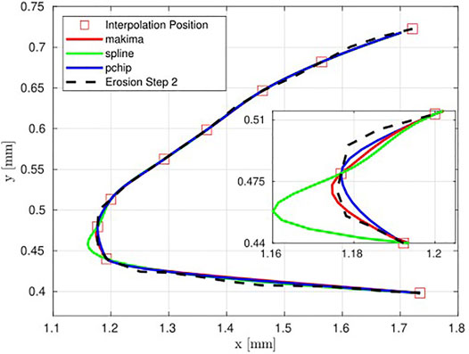
FIGURE 6. Quality of leading-edge reproduction by splines.

6 Cascade Test Rig

The accuracy of the prediction of the local surface set back (Section 4) and the quality of the surface representation (Section 5) are demonstrated using a set of compressor blades eroded in a linear cascade. This allows the real flow field to be approximated to a given degree and to set reproducible experimental boundary conditions (Hirsch, 1993). The advantages of this approach are the moderate complexity of the experiment and the accessibility of the setup to the required set of measurement technologies. However, the combination of in situ erosion and aerodynamic characterization of a cascade of blades places special requirements on the cascade test rig. Movable parts like tailboards and throttles as well as boundary layer suction devices required to adjust the flow field (Hergt et al., 2014; Weber et al., 2002; Serovy and Okiishi, 1988; Lepicovsky et al., 2001; Riffel and Rothrock, 1980) are not applied since particles are introduced into the flow channel for erosion testing. This cascade rig as shown in Figure 7A is based on the one presented in Döring et al. (2017). The rig is supplied with air via a cylindrical plenum featuring two grids to equalize the flow. The airflow is accelerated in a bellmouth intake and enters a rectangular flow section. A turbulence grid consisting of square bars is used to generate turbulence levels equivalent to those in engines (Roach, 1987). A fixed sidewall design suitable for variable incidences (Sokolov et al., 2019) is chosen for the test section. As shown in Figure 7B, it does not require any movable parts. The linear cascade consists of five blades guaranteeing a periodic flow field for the center blade. Arizona A3 Test Dust is fed into the canal with a nozzle protruding into the canal over the blade height at a distance of 660 mm in front of the leading edge of the center blade. This nozzle is retracted from the canal during probe traversal measurements. The particle-laden air passes through the blade row and leaves the cascade through an exhaust system. The design Mach number of the cascade test rig is Ma = 0.76. The blade row can be rotated in the range of i = 2 ± 5° in increments of 1°.

FIGURE 7

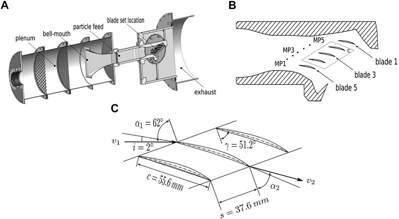
FIGURE 7. Test apparatus (A) with detailed view of the cascade section and the measuring positions (B) and the geometric parameters of the cascade (C).

The blade geometry of the linear cascade shown in Figure 7C is derived from NASA Rotor 37 data (Reid and Moore, 1978; Moore and Reid, 1980) by unwinding it cylindrical at 50% blade height without scaling the blades. Operating conditions typical for idle have been chosen since particle load near the ground is highest (Hobbs, 1993), and a significant amount of blade damage is accumulated during taxi-out and tax-in operations (Brandes et al., 2021). This results in an operation of the cascade at a flow Mach number of Ma = 0.76, an incidence angle of i = +7°, and a particle volume fraction of 1 ⋅ 10^–7.

7 Experimentally Derived Input Data

The particle field impacting the blade surfaces is specific to the given test rig and forms a key input to the numerical computation of the eroded blade geometries. It is experimentally identified to guarantee a consistent result with the particular experimental conditions. Understanding the air flow field allows the interpretation of the observed particle flow field. Flow traverses have been carried out in front of the compressor blade row. Its homogeneity is shown exemplary in Figure 8 for zero incidence conditions.

FIGURE 8

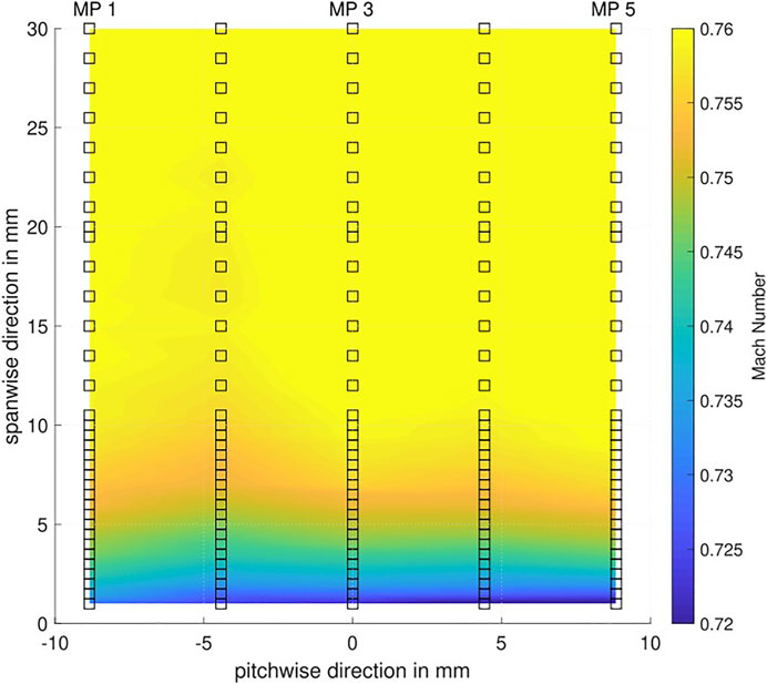
FIGURE 8. Inlet Mach number distribution at i = 0°.

No pitch-wise flow non-homogeneity is evident. Only an expected decay in flow Mach number close to the side wall is observed. Random insertion of particles into this even flow field results in a random distribution of particles of coherent velocities approaching the cascade front. Hence, any observed unevenness of erosive damage to the leading edge of test bodies is related to an uneven distribution of particles. Therefore, the non-homogeneity of the particle distribution typical to the test setup is derived indirectly from the erosive change in the shape of the flat plate specimen replacing the airfoils at their position in the cascade. Featuring the same chord length and blade height, flat plates approximate the flow field of the low camber angle NASA Rotor 37 airfoils reasonably (Scholz and Braun, 1965; Weinig, 1935). They are machined from aluminum alloy EN AW-6060 and are eroded at the same conditions as the blades, namely Ma = 0.76 at i = +7°. The leading-edge step back observed after flat plate erosion is shown in Figure 9A.

FIGURE 9

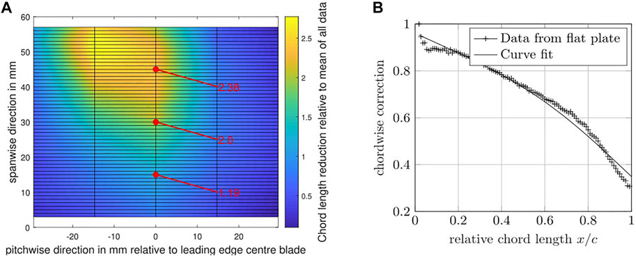
FIGURE 9. Material removal correction at leading edge (A) and at the pressure side (B).

A non-homogeneous change in leading-edge shape is observed peaking at 2/3 span of blades no. 3 and 4. Application of the flat plate erosion rates gives a proportional non-homogeneity in the concentration of the particles. The concentration of particles derived at the leading edge is assumed to prevail in the horizontal flow sections between the flat plates. Due to the measured homogeneous flow field, it is concluded that the non-homogeneity results from the uneven distribution of particles within the channel. Therefore, the mean particle mass flowing through the test sections needs to be scaled to achieve the real particle distribution at the specific position for erosion calculations. Scaling factors for different blade positions are derived from the chord length reduction displayed in Figure 9A. For 25% blade height, the scaling is 1.19, for 50% blade height, it is 2.0, and for 75% blade height, the scaling is 2.38.

Since these scaling factors are only valid for the leading edge of the flat plates, the material loss at the pressure side according to the leading-edge position also needs to be analyzed. The material loss along the pressure side exemplary displayed for blade 3 at 50% height is shown in Figure 9B. The particular erosive condition and the missing observation of erosion on the suction side of the blades support the assumption of a constant impact angle and velocity along surface lines and the neglection of particle rebound. Consequently, the different chord length reductions result from uneven particle distributions along the pressure side. Therefore, a correction of particle concentration along the pressure side relative to the corresponding leading-edge position is applied in the calculations.

Evaluation of the particle distributions at 25, 50, and 75% span at blade 3 provides the boundary conditions for the prediction of the erosive change in blade shape of the cascade of compressor blades. Afterwards, three sets of blades are manufactured from Ti-6Al-4V and experimentally deteriorated under the test conditions mentioned in Section 7. The blades are measured after 4 and 8 kg of sand passed through the facility, defining erosion steps 1 and 2. The erosion steps result in chord length reductions of 1% for erosion step 1 and 2.4% for erosion step 2 at 50% blade height. The chord length reductions correspond to an operational life of about 3,000 to 3,300 flights (Richardson et al., 1979).

8 Parametric Study of Spatial and Time Resolution

The presented method is applied to the erosion of the cascade compressor blades. A parametric study of the segment length and time step is carried out obeying the limits derived above. Calculations are performed with a particle velocity of v = 270 m/s, a profile angle of ψ = 15.8°, and a medium particle distribution of θ = 0.0315 kg/(m²s).

Figure 10 shows the transformation of the profile in Cartesian coordinates toward polar coordinates. The profile is displayed for different circumferential angles starting at the trailing edge and moving in a counterclockwise direction. Polar coordinates are chosen for the representation of the erosion depth.

FIGURE 10

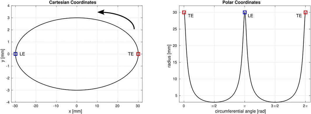
FIGURE 10. Representation of profile in Cartesian coordinates and polar coordinates.

Figure 11 shows the erosion depth normal to the eroded surface for different element sizes computed for blade 3 at 50% blade height and erosion step 2. The peak position at the leading edge between experiment and calculation agrees. On the pressure side, the different element sizes calculate the same erosion depth which is within the experimental uncertainty. The detailed view of the leading edge on the right side of the figure reveals differences between the computations with adjusted element size. While the element size at the limit derived in Section 3 represents the experimental leading edge precisely, the computations worsen with increasing element size resulting in oscillations for an element size of 0.5 mm. The worse prediction for increasing element sizes is due to the geometrical representation of the leading edge. The leading-edge radius is equal to the highest element size. Bigger element sizes are not able to reproduce the leading-edge radius. Therefore, the leading-edge radius determines the upper limit of the element size. An element size of 0.15 mm is preferable.

FIGURE 11

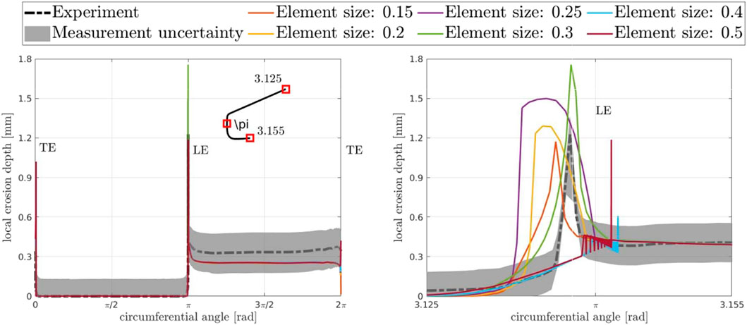
FIGURE 11. Erosion depth for different element sizes.

Figure 12 displays the erosion depth for different time steps for blade 3 at 50% blade height and erosion step 2. The setback is defined through the time step, increasing with the increased time step. All displayed time steps result in a setback smaller than those limited in Section 3. The results on the suction side and pressure side are not influenced by the time step and match the results shown in Figure 11. The influence of the time step is again visible in the detailed view of the leading edge on the right side. The strong peak of the leading edge is not represented for time steps of 500 and 1,000 s. This changes for the time step of 1,500 s. Further increasing the time step worsens the erosion depth calculation due to an increased setback. While all time steps guarantee the particle impact number of 488 impacts, too large setbacks worsen the prediction capability of the method. Therefore, a time step of 1,500 s is preferable for erosion calculations with the presented method.

FIGURE 12

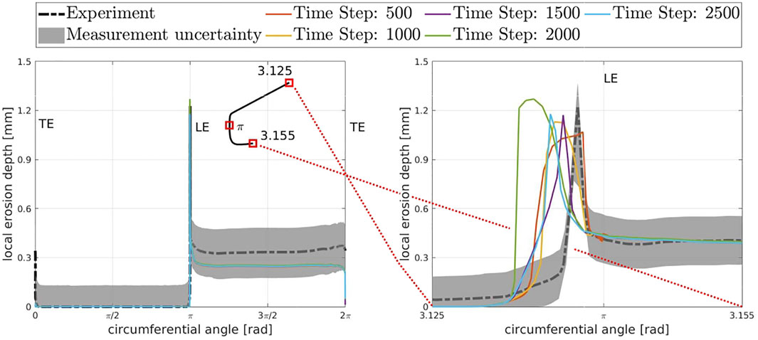
FIGURE 12. Erosion depth for different time steps.

9 Validation Study

Using the preferable values for element size and time step, compressor erosion damage is computed and the results are validated with the experimental values received from the test facility described in Sections 6 and 7.

Erosion predictions for Blade 3 at 25, 50, and 75% blade height with an element size of 0.15 mm and a time step of 1,500 s are displayed in Figure 13 and compared to the experimental results. The non-homogeneous particle distribution explained in Section 7 is considered during the calculations.

FIGURE 13

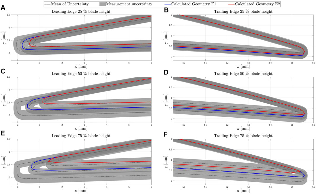
FIGURE 13. Erosion Profile Computation of Blade 3. (A) Leading Edge at 25\% blade height, (B) Trailing Edge at 25\% blade height, (C) Leading Edge at 50\% blade height, (D) Trailing Edge at 50\% blade height, (E) Leading Edge at 75\% blade height and (F) Trailing Edge at 75\% blade height.

Figure A and B show the leading and trailing edge for 25% blade height. The calculation shows typical erosion phenomena such as leading-edge cut back and material removal at the pressure side which are also present in the experiment. The chord length reduction is predicted precisely. The material removal at the pressure side near the trailing edge is within the lower limit of the measurement uncertainty.

Figure C and D show the leading and trailing edge for 50% blade height. Again, the leading edge cut back and the chord length reduction are calculated accurately and in good agreement with the experiment. The material loss at the pressure side meets the experiment within the lower limits at the trailing edge. For this blade, sharpening of the trailing edge resulting from increased material removal is present and meets the experimental observations.

Figure E and F show the leading and trailing edge for 75% blade height. The increased particle concentration is observable through the increased leading edge cut back and increased chord length reduction. Again, the presented method predicts the erosion damage at the leading edge precisely and computes the correct material removal at the pressure side. Increased sharpening of the trailing edge is visible. Both erosion predictions are within the experimental range.

With the discussed limits of spatial and time resolution, the presented method is capable of predicting erosion damage at different blade heights with good accuracy. A prerequisite is an accurate representation of the particular flow field of the investigated erosion case.

10 Conclusion

The application of erosion rates derived as integral parameters from flat plate erosion experiments to cascade compressor blades is presented. The expansion of the dimensional analysis for flat plate erosion experiments documented in Hufnagel et al. (2017) reveals boundary conditions for the spatial and time resolution in erosion computations. The presented meshing procedure is capable of capturing the surface displacement through a spline interpolation that guarantees a correct representation of the geometry. The presented linear cascade erosion experiment is used to derive the validation data. In this experiment, the geometry of NASA Rotor 37 manufactured from Ti-6Al-4V is eroded at an incidence of i = 7° and Ma = 0.76.

The parametric study showed preferable values for the spatial and time resolution of 0.15 mm element length and 1,500 s time step for the computed geometry. The validation study for three representative erosion geometries showed the applicability of the presented erosion computation on eroded cascade compressor blades.

Knowing the local particle transport, the erosion-induced shape change at arbitrary blade geometries can be predicted. The material and experimental parameters underlying the used erosion rate correlations are decisive and may result in values differing from those presented. The computational effectiveness of the approach enables the erosion prediction of more complex and larger components.

Data Availability Statement

The original contributions presented in the study are included in the article/Supplementary Material; further inquiries can be directed to the corresponding author.

Author Contributions

ML, MK, JH, and SS contributed to the conception and design of the study. SS performed the dimensional analysis. ML, MK, JH, and SS contributed to specifying the parameters for spatial and time resolution. JH and MK performed the study for spline representation. ML performed and CK supervised the experimental study. JH performed the optimization study for spatial and time resolution. ML and JH performed the validation study. MK and SS wrote Sections 1–4. JH and SS wrote Sections 5, 8 and 9. ML, JH, and SS wrote Sections 6 and 7. MK, JH, and SS contributed to the manuscript revision and approved the submitted version.

Conflict of Interest

The authors declare that the research was conducted in the absence of any commercial or financial relationships that could be construed as a potential conflict of interest.

Publisher’s Note

All claims expressed in this article are solely those of the authors and do not necessarily represent those of their affiliated organizations, or those of the publisher, the editors, and the reviewers. Any product that may be evaluated in this article, or claim that may be made by its manufacturer, is not guaranteed or endorsed by the publisher.

References

Akima, H. (1970). A New Method of Interpolation and Smooth Curve Fitting Based on Local Procedures. J. Acm 17, 589–602. doi:10.1145/321607.321609

CrossRef Full Text | Google Scholar

Akima, H. (1974). A Method of Bivariate Interpolation and Smooth Surface Fitting Based on Local Procedures. Commun. ACM 17, 18–20. doi:10.1145/360767.360779

CrossRef Full Text | Google Scholar

Balan, C., and Tabakoff, W. (1984). Axial Flow Compressor Performance Deterioration. 20th Joint Propulsion Conference. doi:10.2514/6.1984-1208

CrossRef Full Text | Google Scholar

Bitter, J. G. A. (1963). A Study of Erosion Phenomena Part I. Wear 6, 5–21. doi:10.1016/0043-1648(63)90003-6

CrossRef Full Text | Google Scholar

Bons, J. P., Prenter, R., and Whitaker, S. (2017). A Simple Physics-Based Model for Particle Rebound and Deposition in Turbomachinery. J. Turbomach. 139. doi:10.1115/1.4035921.081009

CrossRef Full Text | Google Scholar

Brandes, T., Koch, C., and Staudacher, S. (2021). Estimation of Aircraft Engine Flight Mission Severity Caused by Erosion. J. Turbomach. 143. doi:10.1115/1.4051000.111001

CrossRef Full Text | Google Scholar

De Boor, C., De Boor, C., Mathématicien, E.-U., De Boor, C., and De Boor, C. (1978). A Practical Guide to Splines, 27. New York: Springer-Verlag.

Google Scholar

Döring, F., Staudacher, S., Koch, C., and Weißschuh, M. (2017). Modeling Particle Deposition Effects in Aircraft Engine Compressors. J. Turbomach. 139, 051003. doi:10.1115/1.4035072

CrossRef Full Text | Google Scholar

Du, M., Li, Z., Feng, L., Dong, X., Che, J., and Zhang, Y. (2021). Numerical Simulation of Particle Fracture and Surface Erosion Due to Single Particle Impact. AIP Adv. 11, 035218. doi:10.1063/5.0042928

CrossRef Full Text | Google Scholar

Hussein, M. F., and Tabakoff, W. (1974). Computation and Plotting of Solid Particle Flow in Rotating Cascades. Comput. fluids 2, 1–15. doi:10.1016/0045-7930(74)90002-4

CrossRef Full Text | Google Scholar

Fritsch, F. N., and Carlson, R. E. (1980). Monotone Piecewise Cubic Interpolation. SIAM J. Numer. Anal. 17, 238–246. doi:10.1137/0717021

CrossRef Full Text | Google Scholar

Ghenaiet, A. (2012). Study of Sand Particle Trajectories and Erosion into the First Compression Stage of a Turbofan. J. Turbomach. 134. doi:10.1115/1.4004750.051025

CrossRef Full Text | Google Scholar

Grant, G., and Tabakoff, W. (1975). Erosion Prediction in Turbomachinery Resulting from Environmental Solid Particles. J. Aircr. 12, 471–478. doi:10.2514/3.59826

CrossRef Full Text | Google Scholar

Grote, K. H., and Feldhusen, J. (2014). Dubbel, Taschenbuch für den Maschinenbau. Berlin Heidelberg: Springer Vieweg.

Google Scholar

Hadavi, V., Moreno, C. E., and Papini, M. (2016). Numerical and Experimental Analysis of Particle Fracture during Solid Particle Erosion, Part I: Modeling and Experimental Verification. Wear 356-357, 135–145. doi:10.1016/j.wear.2016.03.008

CrossRef Full Text | Google Scholar

Hamed, A., Tabakoff, W. C., and Wenglarz, R. V. (2006). Erosion and Deposition in Turbomachinery. J. Propuls. Power 22, 350–360. doi:10.2514/1.18462

CrossRef Full Text | Google Scholar

Hergt, A., Klinner, J., Steinert, W., Grund, S., Beversdorff, M., Giebmanns, a., et al. (2014). The Effect of an Eroded Leading Edge on the Aerodynamic Performance of a Transonic Fan Blade Cascade. J. Turbomach. 137, 021006. doi:10.1115/1.4028215

CrossRef Full Text | Google Scholar

Hirsch, P. C. (1993). Advanced Methods for Cascade Testing. AGARD-AG-328. Neuilly-sur-Seine Cedex: Research and Technology Organisation (NATO).

Google Scholar

Hobbs, P. V. (1993). Aerosol-cloud-climate Interactions. San Diego, CA: Academic Press.

Google Scholar

Hufnagel, M., Staudacher, S., and Koch, C. (2018). Experimental and Numerical Investigation of the Mechanical and Aerodynamic Particle Size Effect in High-Speed Erosive Flows. J. Eng. Gas. Turbines Power 140, 102604. doi:10.1115/1.4039830

CrossRef Full Text | Google Scholar

Hufnagel, M., Werner-Spatz, C., Koch, C., and Staudacher, S. (2017). High-Speed Shadowgraphy Measurements of an Erosive Particle-Laden Jet under High-Pressure Compressor Conditions. J. Eng. Gas. Turbines Power 140, 012604. doi:10.1115/1.4037689

CrossRef Full Text | Google Scholar

Kahaner, D., Moler, C., and Nash, S. (1989). Numerical Methods and Software. NJ: Prentice-Hall.

Google Scholar

Kobryn, P. A., and Semiatin, S. L. (2001). Mechanical Properties of Laser-Deposited Ti-6Al-4V in 2001 International Solid Freeform Fabrication Symposium. doi:10.26153/tsw/3261

CrossRef Full Text

Kopper, P., Beck, A., Ortwein, P., Krais, N., Kempf, D., and Koch, C. (2019). “High-order Large Eddy Simulation of Particle-Laden Flow in a T106C Low-Pressure Turbine Linear Cascade,” in 8th European Conference For Aeronautics And Aerospace Sciences (EUCASS). doi:10.13009/EUCASS2019-1022

CrossRef Full Text | Google Scholar

Lepicovsky, J., Chima, R. V., McFarland, E. R., and Wood, J. R. (2001). On Flowfield Periodicity in the NASA Transonic Flutter Cascade. J. Turbomach. 123, 501–509. doi:10.1115/1.1378300

CrossRef Full Text | Google Scholar

Libertowski, N. D., Geiger, G. M., and Bons, J. P. (2020). Modeling Deposit Erosion in Internal Turbine Cooling Geometries. J. Eng. Gas. Turbines Power 142, 1–9. doi:10.1115/1.4045954

CrossRef Full Text | Google Scholar

Marx, J., Städing, J., Reitz, G., and Friedrichs, J. (2014). Investigation and Analysis of Deterioration in High Pressure Compressors Due to Operation. CEAS Aeronaut. J. 5, 515–525. doi:10.1007/s13272-014-0118-z

CrossRef Full Text | Google Scholar

Marx, W. (2013). Berechnung der Gestaltänderung von Profilen infolge Strahlverschleiß, 76. Berlin Heidelberg: Springer-Verlag.

Google Scholar

Montgomery, D. C., Runger, G. C., and Hubele, N. F. (2004). Engineering Statistics. Hoboken: John Wiley & Sons.

Google Scholar

Moore, R. D., and Reid, L. (1980). Performance of Single-Stage Axial-Flow Transonic Compressor with Rotor and Stator Aspect Ratios of of 1.19 and 1.26, Respectively. NASA TP-16591659

Google Scholar

Mora, A., Alabi, A., and Schmauder, S. (2019). A Lattice Monte Carlo Model for Solid Particle Erosion: An Application to Brittle Fracture. Wear 418-419, 52–60. doi:10.1016/j.wear.2018.10.022

CrossRef Full Text | Google Scholar

Reid, L., and Moore, R. D. (1978). Design and Overall Performance of Highly Loaded, High-Speed Inlet Stages for an Advanced High-Pressure-Ratio Core Compressor. NASA TP-1337, 1–6.

Google Scholar

Richardson, J., Sallee, G., and Smakula, F. (1979). Causes of High Pressure Compressor Deterioration in Service. AIAA, SAE, and ASME, Joint Propulsion Conference.

Google Scholar

Riffel, R. E., and Rothrock, M. D. (1980). Experimental Determination of Unsteady Blade Element Aerodynamics in Cascades. Volume 2: Translation Mode Cascade final report. Indianapolis: Detroit Diesel Allison Division of General Motoros Corporation.

Google Scholar

Roach, P. E. (1987). The Generation of Nearly Isotropic Turbulence by Means of Grids. Int. J. Heat Fluid Flow 8, 82–92. doi:10.1016/0142-727x(87)90001-4

CrossRef Full Text | Google Scholar

Sallee, G. P. (1978). Performance Deterioration Based on Existing (Historical) Data- JT9D Jet Engine Diagnostics Program. NASA CR 135448, 225doi. doi:10.1016/j.applanim.2005.06.011

CrossRef Full Text | Google Scholar

Scholz, N., and Braun, G. (1965). “Aerodynamik der Schaufelgitter,” in No. Bd. 1 in Wissenschaftliche Bücherei : Reihe Strömungstechnik.

Google Scholar

Schrade, M., Staudacher, S., and Voigt, M. (2015). Experimental and Numerical Investigation of Erosive Change of Shape for High-Pressure Compressors. In Turbo Expo: Power for Land, Sea, and Air. American Society of Mechanical Engineers, 1–9. doi:10.1115/GT2015-42061

CrossRef Full Text | Google Scholar

Schrade, M. (2015). Untersuchungen zum Einfluss des Strahlverschleißes auf Hochdruckverdichterschaufeln von Turboflugtriebwerken. Universität Stuttgart: Ph.D. thesis.

Google Scholar

Serovy, G. K., and Okiishi, T. H. (1988). Performance of a Compressor Cascade Configuration with Supersonic Entrance Flow - a Review and Comparison of Experiments in Three Installations. J. Turbomach. 110, 441–449. doi:10.1115/1.3262217

CrossRef Full Text | Google Scholar

Sokolov, M., Lorenz, M., Rostamian, M., Koch, C., Weissschuh, M., and Staudacher, S. (2019). Advances in High-Speed Linear Design Technology: Novel Approach to Sidewall Geometry Design for Erosion Tests. Turbo Expo Power Land, Sea, Air 58554, V02AT39A015. doi:10.1115/gt2019-90743

CrossRef Full Text | Google Scholar

Sommerfeld, H., Koch, C., Schwarz, A., and Beck, A. (2021). High Velocity Measurements of Particle Rebound Characteristics under Erosive Conditions of High Pressure Compressors. Wear 470-471, 203626. doi:10.1016/j.wear.2021.203626

CrossRef Full Text | Google Scholar

Weber, A., Schreiber, H.-A., Fuchs, R., and Steinert, W. (2002). 3-D Transonic Flow in a Compressor Cascade With Shock-Induced Corner Stall. J. Turbomach. 124, 358–366. doi:10.1115/1.1460913

CrossRef Full Text | Google Scholar

Weinig, F. (1935). Die Strömung um die Schaufeln von Turbomaschinen: Beitrag zur Theorie axial durchströmter Turbomaschinen (Barth)München: Barth.

Google Scholar

Wong, C. Y., Solnordal, C., Swallow, A., Wang, S., Graham, L., and Wu, J. (2012). Predicting the Material Loss Around a Hole Due to Sand Erosion. Wear 276-277, 1–15. doi:10.1016/j.wear.2011.11.005

CrossRef Full Text | Google Scholar

Glossary

Latin Letters

A surface element

d diameter

da element length

db element width

dh element height

E Young’s modulus

e erosion rate

F function

f frequency

H_v hardness

i incidence

l displacement depth

m mass

Ma Mach number

q Poissons’s ratio

R_p0,2 yield strength

T temperature

t time step

V volume

v velocity

y elastic load limit.

Indices and Accent Marks

()_1,2,3 numbering

()_el elastic

()_I impact

()_M surface material

()_max maximum

()_min minimum

()_melt melting

()_n normal

()_observed observed

()_Sand sand

()_P particle

()_p plastic

()_t tangential

$\acute{()}$ modified parameter

$\dot{()}$ time derivative.

Greek Letters

Δ increment

θ particle distribution

ξ impact angle

Π nondimensional group

ρ density

σ standard deviation

χ goodness of fit

Ψ profile angle.

German Letters

L spatial dimension

M mass dimension

T temperature dimension

t time dimension.