Large-eddy simulation of a 15 GW wind farm: Flow effects, energy budgets and comparison with wake models

1 Introduction

The installed offshore wind power in Europe is expected to grow significantly in the next three decades due to high offshore wind targets of several countries. For example, the four countries Belgium, Denmark, Germany and the Netherlands defined an offshore wind target of 150 GW for the year 2050 in the Esbjerg declaration (Frederiksen et al., 2022). The wind farm clusters that are required to achieve this target will have a rated power on the order of 10 GW as the offshore wind plans for Germany show (BSH, 2022).

An efficient wind farm cluster design can only be achieved if the layout optimization and yield estimation is done with simulation tools that deliver accurate results. Due to the large number of possible combinations between wind speed, wind direction, farm layout and other parameters, these simulations can only be performed with computationally inexpensive analytical wake models. However, analytical wake models are tuned with data of existing wind farms that are much smaller than the planned wind farm clusters. The wake models might thus not be suitable for predicting the power output of large wind farm clusters. A sound method to investigate the wake flow and power output of large potential wind farms is large-eddy simulation (LES). With LES all relevant processes such as turbulent entrainment of energy or Coriolis effects are modeled. Many wind farm LES studies have been performed in recent years, e.g., Allaerts and Meyers (2017), Wu and Porté-Agel (2017), Zhang et al. (2019), Centurelli et al. (2021), Lanzilao and Meyers (2022) and Maas and Raasch (2022). They show that complex flow phenomenon like inversion layer displacement, gravity wave induced pressure gradients, flow blockage and Coriolis force related wind direction changes can occur for large wind farms. Analytical wake models do not account for these effects which might result in large errors in the power prediction. Currently there is no LES study of a multi-gigawatt wind farm that compares the results with analytical wake models.

The aim of this study is to fill this research gap by comparing two analytical wake models with a large-eddy simulation of a 15 GW wind farm. The NP model (Niayifar and Porté-Agel, 2016) and the TurbOPark model (Pedersen et al., 2022) are chosen because they use a Gaussian wake profile and a turbulence model. Potential discrepancies in the power output are identified and explained by an energy budget analysis. The LES model domain has a size of 245 km × 138 km × 8 km and is filled with a turbine wake resolving grid resulting in 6.8 billion grid points in total. The wind farm has a finite size in both lateral directions unlike in many other studies in which the wind farm is effectively infinitely wide in the crosswise direction (e.g., Stevens et al., 2016; Allaerts and Meyers, 2017; Maas, 2022b). The LES results are compared with the infinitely wide wind farm case of Maas (2022b) to show which new flow effects occur if the more realistic finite size wind farm setup is used.

The paper is structured as follows: The LES model and simulation setup are described in Section 2. The results are presented in Section 3, and Section 4 concludes and discusses the results of the study.

2 Materials and methods

2.1 Numerical model

The large-eddy simulation is carried out with the Parallelized Large-eddy Simulation Model PALM (Maronga et al., 2020). PALM is developed at the Institute of Meteorology and Climatology of the Leibniz Universität Hannover, Germany. Several wind farm flow investigations have been successfully conducted with this code in the past (e.g., Witha et al., 2014; Dörenkämper et al., 2015; Krüger et al., 2022; Maas and Raasch, 2022). PALM solves the non-hydrostatic, incompressible Navier-Stokes equations in Boussinesq-approximated form. The equations for the conservation of mass, momentum and internal energy are:

$\frac{\partial {\tilde{u}}_j}{\partial x_j}=0,(1)$

$\frac{\partial {\tilde{u}}_i}{\partial t}=-\frac{\partial {\tilde{u}}_i{\tilde{u}}_j}{\partial x_j}-{ϵ}_{\mathit{ijk}}{f}_j{\tilde{u}}_k+{ϵ}_{i3j}{f}_3{u}_{g,j}-\frac{1}{{\rho }_0}\frac{\partial {\pi }^{*}}{\partial x_i}+g\frac{\tilde{\theta }-\langle \tilde{\theta }\rangle }{\langle \tilde{\theta }\rangle }{\delta }_{i3}-\frac{\partial }{\partial x_j}\left(\widetilde{u_i^{\prime \prime }{u}_j^{\prime \prime }}-\frac{2}{3}e{\delta }_{ij}\right)+d_i,(2)$

$\frac{\partial \tilde{\theta }}{\partial t}=-\frac{\partial {\tilde{u}}_j\tilde{\theta }}{\partial x_j}-\frac{\partial }{\partial x_j}\left(\widetilde{u_j^{\prime \prime }{\theta }^{\prime \prime }}\right),(3)$

where angular brackets indicate horizontal averaging, a double prime indicates subgrid-scale (SGS) quantities, a tilde denotes filtering over a grid volume, i, j, k ∈ {1, 2, 3}, u_i, u_j, u_k are the velocity components in the respective directions (x_i, x_j, x_k), θ is potential temperature, t is time, f_i = (0, 2Ω cos(ϕ), 2Ω sin(ϕ)) is the Coriolis parameter with the Earth’s angular velocity Ω = 0.729 × 10⁻⁴ rad·s⁻¹ and the geographical latitude ϕ. The geostrophic wind speed components are u_g,j and the basic state density of dry air is ρ₀. The modified perturbation pressure is ${\pi }^{*}=p+\frac{2}{3}{\rho }_{0}e$, where p is the perturbation pressure and $e=\frac{1}{2}\widetilde{u_i^{\prime \prime }{u}_i^{\prime \prime }}$ is the SGS turbulence kinetic energy. The gravitational acceleration is g = 9.81 m·s⁻², δ is the Kronecker delta and d_i are the forces of the wind turbine actuator discs.

The SGS model uses a 1.5-order closure according to Deardorff (1980), modified by Moeng and Wyngaard (1988) and Saiki et al. (2000). The numerical grid is a structured, equidistant, staggered Arakawa C-grid that can be vertically stretched above a certain height.

The wind turbines are represented by an advanced actuator disc model with rotation (ADM-R) that acts as an axial momentum sink and an angular momentum source (inducing wake rotation). The ADM-R is described in detail by Wu and Porté-Agel (2011) and was implemented in PALM by Steinfeld et al. (2015). Additional information is also given by Maas and Raasch (2022). The wind turbines have a yaw controller, that aligns the rotor axis with the wind direction.

2.2 Main simulation

The wind farm consists of 32 × 32 = 1,024 wind turbines. The IEA 15 MW wind turbine with a rotor diameter of D = 240 m and a rated power of 15 MW is used (Gaertner et al., 2020). The hub height is set to 180 m instead of 150 m, so that the turbulent fluxes at the rotor bottom are better resolved by the numerical grid. The turbine spacing in the streamwise and crosswise direction is s_x = s_y = 6 D, resulting in an installed power density of 7.23 W·m⁻², which is a typical value for currently planned offshore wind farms in the German Bight (BSH, 2022). The wind turbines are arranged in a staggered configuration, i.e., every second row is shifted by s_y/2 in the y-direction. The wind farm has a size of l_x × l_y = 44.64 km × 45.36 km.

The numerical grid has a size of N_x × N_y × N_z = 12,288 × 6,912 × 80 ≈ 6.8 × 10⁹ grid points. The grid spacing is Δx = Δy = Δz = 20 m, corresponding to 12 grid points per rotor diameter. With this grid spacing the ratio of SGS-TKE to total TKE (SGS and resolved TKE) is below 20% in the wind turbine wakes, except for the first two columns, where it reaches values of approximately 30%. Above z = 700 m, in the non-turbulent free atmosphere, the grid is stretched vertically by 8% every grid level up to Δz_max = 400 m. This results in a domain size of L_x × L_y × L_z = 245.76 km × 138.24 km × 8.28 km (see Figure 1). The large domain height is needed to cover at least one vertical wavelength of the stationary gravity waves (5.3 km) that form in the free atmosphere above the wind farm (refer to Allaerts and Meyers (2017) for details). To avoid the reflection of gravity waves at the domain top, there is a Rayleigh damping layer above z_rd = 4.5 km. In this damping layer the velocity components are damped towards their respective inflow value by subtracting a tendency that is proportional to the deviation from the inflow value. The magnitude of the damping is given by the Rayleigh damping factor that increases from zero at the bottom of the damping layer to its maximum value of f_rdm = 0.025(Δt)⁻¹ ≈ 0.017 s⁻¹ at the domain top according to this function (see Figure 1):

$f_{rd}\left(z\right)=f_{\mathit{rdm}}{\sin }^2\left(0.5\pi \frac{z-z_{rd}}{L_z-z_{rd}}\right).(4)$

This sine wave profile leads to less reflections compared to a linear profile (Klemp and Lilly, 1978).

FIGURE 1

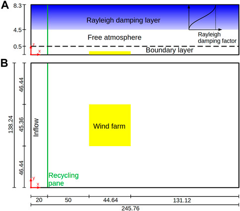
FIGURE 1. (A) Side view of the domain layout. Inside the Rayleigh damping layer the damping factor increases according to the sin²-function in Eq. 4. (B) Plan view of the domain layout. Dimensions in km.

The flow field is initialized by the instantaneous flow field of the last time step of a precursor simulation. Details about the precursor simulation and the meteorological parameters are given in the next section. The flow field is filled cyclically into the main domain, because it is larger than the precursor domain. At the inflow, vertical profiles of the potential temperature and the velocity components averaged over the last 4 h of the precursor simulation are prescribed (see Figure 2). The turbulent state of the inflow is maintained by a turbulence recycling method that maps the turbulent fluctuations from the recycling plane at x = 20 km onto the inflow plane at x = 0. The turbulent fluctuations are shifted in the y-direction by +53.76 km to avoid streamwise streaks in the averaged velocity fields, for further details please refer to Munters et al. (2016). More details of the recycling method are provided in Maas and Raasch (2022). The wind farm has a distance of 50 km to the recycling plane to reduce the influence of the wind farm flow blockage on the flow at the recycling plane. To avoid an artificial formation of gravity waves at the inflow boundary, there is a second Rayleigh damping zone between x = 0 and x = 10 km. The damping mechanism is the same as in the Rayleigh damping layer except that it only acts on the potential temperature field. The damping factor has a magnitude of f_ptm = 0.025(Δt)⁻¹ ≈ 0.017 s⁻¹ at the inflow boundary and decreases to zero at x = 10 km according to the sine wave profile in Eq. 4.

FIGURE 2

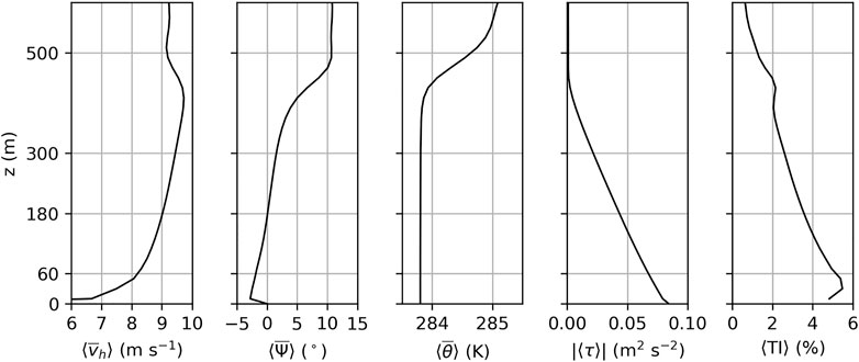
FIGURE 2. Vertical profiles of the horizontal wind speed v_h, the wind direction Ψ (clockwise positive), the potential temperature θ, the kinematic momentum flux τ and the turbulence intensity TI. The profiles are horizontally averaged (⟨•⟩) over the entire precursor domain and temporally averaged $(\overline{•})$ over the last 4 h of the precursor simulation. Horizontal lines mark rotor bottom (60 m), hub height (180 m), rotor top (300 m) and inversion layer height (500 m).

Cyclic boundary conditions are applied at the northern and southern domain boundaries (y-direction). Radiation boundary conditions as described by Miller and Thorpe (1981) and Orlanski (1976) are applied at the outflow (right) domain boundary. At the domain top and bottom a Neumann boundary condition for the perturbation pressure and Dirichlet boundary conditions for the velocity components are applied. For the potential temperature, a constant lapse rate is assumed at the domain top. The physical simulation time of the main simulation is 24 h and the presented data are averaged over the last 4 h. The simulation ran on 5,184 cores for a wall-clock time of 50 h.

2.3 Precursor simulation

Initial conditions and inflow profiles are obtained by a precursor simulation that does not contain a wind farm. It has cyclic boundary conditions in both lateral directions and a domain size of L_x,pre × L_y,pre × L_z,pre = 3.84 km × 2.24 km × 8.3 km. The number of vertical grid points, the vertical grid stretching and Rayleigh damping levels are the same as in the main simulation. The initial horizontal velocity is set to the geostrophic wind (U_g, V_g) = (9.064, −1.722) m·s⁻¹, resulting in a steady-state hub height mean wind speed of 9.0 m·s⁻¹ that is aligned with the x-axis. The latitude is ϕ = 55°N. The initial potential temperature is set to 283 K at the surface and has a lapse rate of Γ = +3.5 K·km⁻¹ above. The onset of turbulence is triggered by small random perturbations in the horizontal velocity field below a height of 250 m in the entire precursor domain at the first time step. The amplitude of the perturbations is set to 0.25 m·s⁻¹. The roughness length is z₀ = 1 mm and a constant flux layer is assumed between the surface and the lowest computational grid level. The heat flux at the surface is set to zero so that a conventionally neutral boundary layer with a final boundary layer height of h ≈ 500 m develops. The physical simulation time of the precursor simulation is 48 h. Figure 2 shows temporally and horizontally averaged profiles of the horizontal wind speed v_h, the wind direction Ψ, the potential temperature θ, the total turbulent vertical kinematic momentum flux τ and the turbulence intensity (TI):

$\text{TI}=\frac{\sqrt{\frac{2}{3}\text{TKE}}}{\overline{v_h}},(5)$

with the turbulence kinetic energy (TKE) defined as the sum of the resolved and the SGS-TKE:

$\text{TKE}=\frac{1}{2}\left(\overline{u^{\prime 2}}+\overline{v^{\prime 2}}+\overline{w^{\prime 2}}\right)+\bar{e},(6)$

where u′, v′ and w′ are the deviations from the temporal mean quantity of the resolved flow, e.g., $u^{\prime }=u-\bar{u}$. The temporal mean is used instead of the horizontal mean so that the TKE can be computed at every grid point.

3 Results

3.1 Mean flow at hub height

Figure 3A shows the mean horizontal wind speed at hub height. In general, the flow field shows the typical wind farm flow features such as flow blockage in front of the wind farm, a significant speed deficit inside the wind farm and a slow wind speed recovery in the wake. The flow is decelerated from 9 m·s⁻¹ to below 8 m·s⁻¹ upstream of the wind farm, is further reduced to below 5.5 m·s⁻¹ inside the wind farm and recovers to more than 8 m·s⁻¹ in the wake. However, there are also some remarkable features such as horizontal divergence, flow deflection and wake narrowing.

FIGURE 3

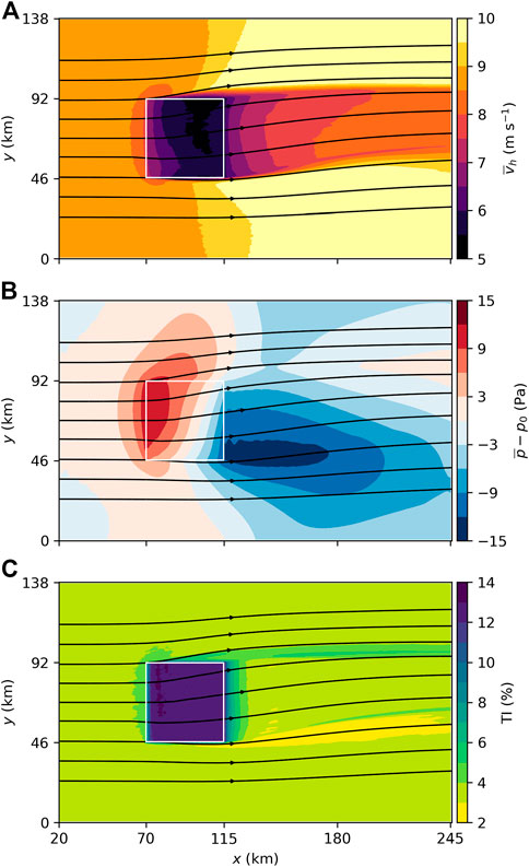
FIGURE 3. Horizontal cross sections of the mean horizontal wind speed (A), the mean perturbation pressure (B) and the turbulence intensity (C) averaged over the last 4 h of the 24 h simulation time. An additional rolling average with a window size of one turbine spacing in x- and y-direction is applied to all quantities to facilitate the interpretation. The borders of the wind farm are marked by white lines.

The flow diverges in the crosswise direction, resulting in a wind direction change of −4° at the northwestern and +2° at the southwestern wind farm corner. The divergence is caused by a high pressure region of approximately +12 Pa near the wind farm leading edge (see Figure 3B).

The second remarkable feature is the narrowing of the wake. Using a wind speed threshold of 8.5 m·s⁻¹, the initial wake width at x = 120 km (5.36 km behind the last turbine) is δ_w = 51 km. This is wider than the wind farm itself (45.36 km) because the wake flow also leaves the northern wind farm edge. Further downstream the wake narrows to δ_w = 43 km and δ_w = 38 km at x = 180 km and x = 240 km, respectively. The wake narrowing (crosswise convergence) is caused by the flow acceleration (streamwise divergence) in the wake. The vertical divergence/convergence has no significant contribution to the wake narrowing (analysis not shown).

The flow divergence and wake narrowing do not occur for smaller wind farms, such as the Horns Rev offshore wind farm (Porté-Agel et al., 2020). These effects do also not occur in simulation setups in which the wind farm is effectively infinitely wide in the cyclic y-direction, such as in Stevens et al. (2016), Allaerts and Meyers (2017), Wu and Porté-Agel (2017) and Maas (2022b).

The third remarkable feature is the counterclockwise deflection of the flow that reaches a maximum of approximately −8° at the center of the trailing edge of the wind farm. As shown by Maas and Raasch (2022) and Maas (2022b) this deflection is caused by a reduction of the Coriolis force in the wind speed deficit region and occurs for wind farm flows for which the Rossby number is on the order of 1 or smaller. The Rossby number in this study is

$Ro=\frac{U_g}{l_{x}f}=\frac{9\mathrm{m}{\mathrm{s}}^{-\mathrm{1}}}{45\mathrm{k}\mathrm{m}\times 1.2\times 10^{-4}}\approx 1.7,(7)$

which is close to 1 and thus flow deflection occurs. The combination of the divergence and the flow deflection results in a wind direction change of more than −10° in the northern part of the wind farm. In the wake, the wind direction turns back clockwise and at the outflow boundary it reaches the initial value of the inflow. The clockwise wake turning has also been shown by Maas (2022b) for an infinitely wide wind farm, where it was related to supergeostrophic wind speeds in the wake due to an inertial oscillation. But in this study the wind speed in the wake does not become supergeostrophic. The clockwise deflection in the wake is rather a result of the pressure distribution.

The pressure distribution (see Figure 3B) generally has the expected pattern with a high pressure region in the upstream part of the wind farm and a low pressure region in the wake. The streamwise variation in the pressure is related to stationary gravity waves in the stably stratified free atmosphere that are described in the next section. However, in the wake the pressure distribution has a high asymmetry in the y-direction with higher pressure at the northern wake edge and lower pressure at the southern wake edge. This crosswise pressure gradient results in a southward pointing tendency so that the wind direction in the wake turns clockwise and adjusts to the wind direction of the surrounding flow. Also the high pressure region in the upstream part of the wind farm is not symmetric. This is the result of the fact that the flow in the free atmosphere is veered by approximately 10° to the right relative to the flow at hub height (see Figure 2). Thus the gravity wave related pressure field is also rotated by 10° to the right.

Figure 3C shows the TI at hub height. The ambient TI at hub height is approximately 3.5% (see also Figure 2). Upstream of the wind farm there is a slight increase in TI which is caused by the reduction in wind speed rather than an increase in TKE (see Eq. 5). Inside the wind farm the TI increases to more than 12% within two turbine columns and is approximately constant up to the trailing edge of the wind farm. In the wake the TI drops to below 5% within 10 km. At the northern wake edge the TI stays at a higher level (approx. 5%) and at the southern wake edge the TI drops to below 3%. It is not yet fully understood why these streaks of higher and lower TI occur and why they persist for over 100 km.

3.2 Inversion layer displacement and gravity waves

The flow deceleration inside the wind farm does not only cause a crosswise divergence but also a vertical divergence. Consequently, the inversion layer is displaced upwards, as can be seen in Figure 4. Here, the inversion layer displacement is defined as the inversion layer height relative to the inversion layer height at the recycling plane at x = 20 km:

$\delta =z_i-{⟨z_i\left(x=20\mathrm{k}\mathrm{m}\right)⟩}_y.(8)$

The inversion layer height is defined as the height at which the maximum vertical potential temperature gradient occurs. The maximum displacement of +120 m occurs in the north-eastern part of the wind farm, where also the minimum wind speed at hub height occurs. In the wake, the inversion layer displacement is very asymmetric with positive values in the northern part and negative values in the southern part. This asymmetry is caused by the wake deflection that leads to a crosswise convergence and thus ascending motion in the northern part of the wake and to a crosswise divergence and thus descending motion in the southern part of the wake (not shown). On average, there is a positive inversion layer displacement in the wake.

FIGURE 4

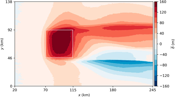
FIGURE 4. Inversion layer displacement. A rolling average with a window size of one turbine spacing in x- and y-direction is applied. The borders of the wind farm are marked by white lines.

The inversion layer displacement triggers gravity waves in the overlying free atmosphere, as described by, e.g., Allaerts and Meyers (2017) and Maas (2022b). The gravity waves affect the velocity, pressure and temperature fields. A detailed discussion of the gravity waves is beyond the scope of this study. Thus, only one vertical cross-section of the perturbation pressure in the center of the wind farm is shown in Figure 5. It shows that the pressure distribution in the wind farm (see Figure 3B) is related to the above lying gravity waves. The waves have upstream inclined phase lines indicating upwards propagating energy. The Rayleigh damping layer reduces the reflectivity of the upper domain boundary to less than 10%. The reflectivity is obtained by the method described by Allaerts and Meyers (2017), which is a modified version of the method described by Taylor and Sarkar (2007).

FIGURE 5

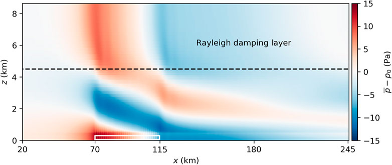
FIGURE 5. Mean perturbation pressure in a vertical cross section through the center of the wind farm. The pressure is given as deviation from the pressure at the inflow at the same height (p₀).

3.3 Energy budget analysis

In this section the kinetic energy budgets inside the wind farm are investigated in detail. The results can be used to explain potential discrepancies between the wake models and PALM in the next section. Additionally, it is possible to quantify the effect of the lateral (south/north) wind farm boundaries on the wind farm energy budgets by comparing the results with semi-infinite wind farm LES studies. The analysis is very similar to the energy budget analysis made by Allaerts and Meyers (2017); Maas (2022b) but is extended to also cover the energy fluxes through the south/north boundaries of the wind farm. These are net zero in the aforementioned studies due to the cyclic boundary conditions at the south/north boundaries of the domain and because the wind farm extends over the entire domain in the y-direction. The energy budgets are calculated for 16 × 16 = 256 wind turbine control volumes Ω_wt. Each control volume (CV) covers 4 wind turbines as sketched in Figure 6. The CVs have a streamwise and crosswise length of 2 turbine spacings. The bottom and top boundaries of Ω_wt are (z_b, z_t) = (50, 310) m, which is 1 dz larger than the rotor diameter, to cover the smeared forces of the wind turbine model. The sum of all wind turbine CVs gives the wind farm CV Ω_wf = ΣΩ_wt.

FIGURE 6

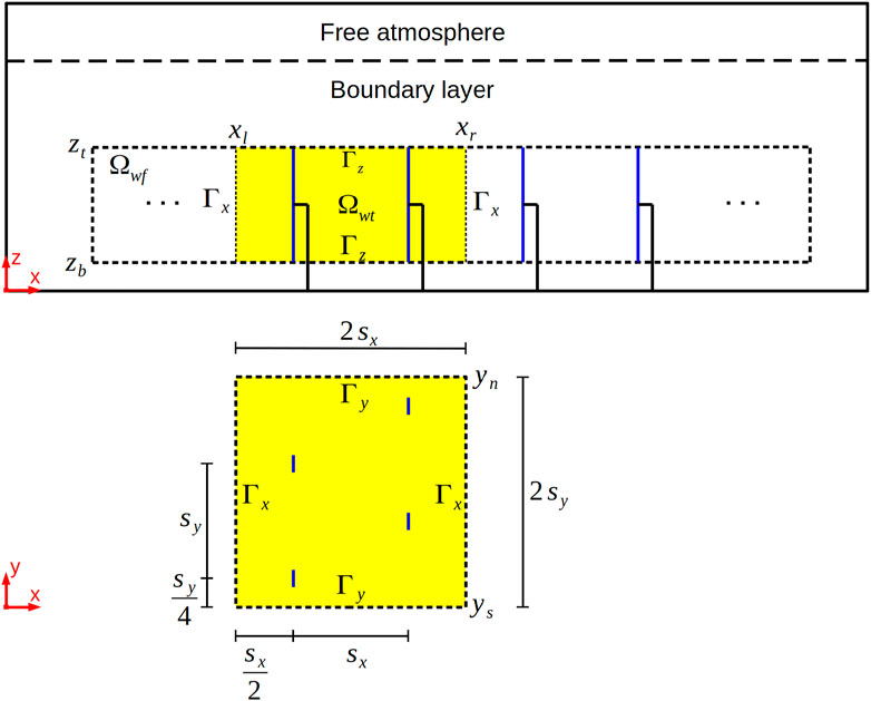
FIGURE 6. Sketch of the wind turbine control volumes Ω_wt and the wind farm control volume Ω_wf. In x-direction the control volumes are bounded by the boundaries Γ_x at x = x_l (left) and x = x_r (right). In the vertical direction, the control volumes are bounded by Γ_z at z = z_b (bottom) and z = z_t (top). In y-direction the control volumes are bounded by Γ_y at y = y_s (south) and y = y_n (north).

The equation for the conservation of the mean resolved-scale kinetic energy can be obtained by multiplying PALM’s equation for momentum conservation (Eq. 2) with u_i, averaging in time, assuming stationarity and integrating over the CV Ω:

$\begin{array}{cc}\hfill 0& =\underset{\mathcal{A}}{\underbrace{-{\int }_{\mathrm{\Omega }}\frac{\partial {\overline{\stackrel{̃}{u}}}_j{\bar{E}}_k}{\partial x_j}d\mathrm{\Omega }}}\underset{\mathcal{F}}{\underbrace{-{\int }_{\mathrm{\Omega }}\frac{\partial }{\partial x_j}{\overline{\stackrel{̃}{u}}}_i\overline{{\stackrel{̃}{u}}_i^{\prime }{\stackrel{̃}{u}}_j^{\prime }}d\mathrm{\Omega }+{\int }_{\mathrm{\Omega }}\frac{\partial }{\partial x_j}\overline{{\stackrel{̃}{u}}_i{\tau }_{ij}}d\mathrm{\Omega }-{\int }_{\mathrm{\Omega }}\frac{\partial }{\partial x_j}\frac{1}{2}\overline{{\stackrel{̃}{u}}_j^{\prime }{\stackrel{̃}{u}}_i^{\prime }{\stackrel{̃}{u}}_i^{\prime }}d\mathrm{\Omega }-{\int }_{\mathrm{\Omega }}\stackrel{̄}{\frac{{\tilde{u}}_i^{\prime }}{{\rho }_0}\frac{\partial {\pi }^{*\prime }}{\partial x_i}}d\mathrm{\Omega }}}\hfill \\ \hfill & \underset{\mathcal{G}}{\underbrace{+{\int }_{\mathrm{\Omega }}\left({\overline{\stackrel{̃}{u}}}_2{f}_3{u}_{g,1}-{\overline{\stackrel{̃}{u}}}_1{f}_3{u}_{g,2}\right)d\mathrm{\Omega }}}\underset{\mathcal{P}}{\underbrace{-{\int }_{\mathrm{\Omega }}\frac{{\overline{\stackrel{̃}{u}}}_i}{{\rho }_0}\frac{\partial \overline{{\pi }^{*}}}{\partial x_i}d\mathrm{\Omega }}}\underset{\mathcal{B}}{\underbrace{+{\int }_{\mathrm{\Omega }}\frac{g}{{\theta }_0}\overline{\left(\stackrel{̃}{\theta }-{\theta }_0\right){\stackrel{̃}{u}}_3}d\mathrm{\Omega }}}\hfill \\ \hfill & \underset{\mathcal{D}}{\underbrace{-{\int }_{\mathrm{\Omega }}\stackrel{̄}{{\tau }_{ij}\frac{\partial {\tilde{u}}_i}{\partial x_j}}d\mathrm{\Omega }-\mathcal{R}}}\underset{\mathcal{W}}{\underbrace{+{\int }_{\mathrm{\Omega }}\overline{{\stackrel{̃}{u}}_i{d}_i}d\mathrm{\Omega }}},\hfill \end{array}(9)$

Note that the mean kinetic energy (KE, ${\bar{E}}_k$) contains the kinetic energy of the mean flow and the turbulence kinetic energy (TKE) of the resolved flow:

${\bar{E}}_k=\frac{1}{2}\overline{{\stackrel{̃}{u}}_i{\stackrel{̃}{u}}_i}=\frac{1}{2}{\overline{\stackrel{̃}{u}}}_i{\overline{\stackrel{̃}{u}}}_i+\frac{1}{2}\overline{{\stackrel{̃}{u}}_i^{\prime }{\stackrel{̃}{u}}_i^{\prime }}(10)$

The terms of Eq. 9 are categorized as follows:

$\mathcal{A}$: Divergence of KE advection

$\mathcal{F}$: Turbulent fluxes

$\mathcal{G}$: Energy input by the geostrophic forcing

$\mathcal{P}$: Energy input by mean perturbation pressure gradients

$\mathcal{B}$: Energy input by buoyancy forces

$\mathcal{D}$: Dissipation by SGS model less the residual $\mathcal{R}$

$\mathcal{W}$: Energy extraction by the wind turbines

The turbulent fluxes $(\mathcal{F})$ can be subdivided into the transport of kinetic energy of the mean flow by resolved turbulent stresses (term 1), transport of KE by SGS stresses (term 2), turbulent transport of resolved-scale TKE by velocity fluctuations (term 3) and turbulent transport of KE by perturbation pressure fluctuations (term 4). Eq. 9 has a positive residual $\mathcal{R}$, because the magnitude of the calculated dissipation is underestimated, which has two reasons: First, the local velocity gradients are underestimated, because they are calculated with central differences. Second, the fifth order upwind advection scheme of Wicker and Skamarock (2002) has numerical dissipation, suppressing the magnitude of the smallest eddies, for which the gradients and the dissipation are highest (Maronga et al., 2013). The positive residual is subtracted from the negative dissipation term $\mathcal{D}$ to compensate for the underestimated magnitude of the calculated dissipation.

Instead of calculating terms $\mathcal{A}$ and $\mathcal{F}$ as a volume integral, they can also be calculated as a surface integral over the CV boundaries (Gauss’s theorem):

$\mathcal{A}=\underset{{\mathcal{A}}_x}{\underbrace{{\left[{\int }_{{\mathrm{\Gamma }}_x}\left(-{\overline{\stackrel{̃}{u}}}_1{\bar{E}}_k\right)d{\mathrm{\Gamma }}_x\right]}_{x_l}^{x_r}}}+\underset{{\mathcal{A}}_y}{\underbrace{{\left[{\int }_{{\mathrm{\Gamma }}_y}\left(-{\overline{\stackrel{̃}{u}}}_2{\bar{E}}_k\right)d{\mathrm{\Gamma }}_y\right]}_{y_s}^{y_n}}}+\underset{{\mathcal{A}}_z}{\underbrace{{\left[{\int }_{{\mathrm{\Gamma }}_z}\left(-{\overline{\stackrel{̃}{u}}}_3{\bar{E}}_k\right)d{\mathrm{\Gamma }}_z\right]}_{z_b}^{z_t},}}(11)$

$\begin{array}{cc}\hfill \mathcal{F}& =\underset{{\mathcal{F}}_x}{\underbrace{{\left[{\int }_{{\mathrm{\Gamma }}_x}\left(-{\overline{\stackrel{̃}{u}}}_i\overline{{\stackrel{̃}{u}}_i^{\prime }{\stackrel{̃}{u}}_1^{\prime }}+\overline{{\stackrel{̃}{u}}_i{\tau }_{i1}}-\frac{1}{2}\overline{{\stackrel{̃}{u}}_1^{\prime }{\stackrel{̃}{u}}_i^{\prime }{\stackrel{̃}{u}}_i^{\prime }}-\frac{\overline{{\stackrel{̃}{u}}_1^{\prime }{\pi }^{*\prime }}}{{\rho }_0}\right)d{\mathrm{\Gamma }}_x\right]}_{x_l}^{x_r}}}\hfill \\ \hfill & +\underset{{\mathcal{F}}_y}{\underbrace{{\left[{\int }_{{\mathrm{\Gamma }}_y}\left(-{\overline{\stackrel{̃}{u}}}_i\overline{{\stackrel{̃}{u}}_i^{\prime }{\stackrel{̃}{u}}_2^{\prime }}+\overline{{\stackrel{̃}{u}}_i{\tau }_{i2}}-\frac{1}{2}\overline{{\stackrel{̃}{u}}_2^{\prime }{\stackrel{̃}{u}}_i^{\prime }{\stackrel{̃}{u}}_i^{\prime }}-\frac{\overline{{\stackrel{̃}{u}}_2^{\prime }{\pi }^{*\prime }}}{{\rho }_0}\right)d{\mathrm{\Gamma }}_y\right]}_{y_s}^{y_n}}}\hfill \\ \hfill & +\underset{{\mathcal{F}}_z}{\underbrace{{\left[{\int }_{{\mathrm{\Gamma }}_z}\left(-{\overline{\stackrel{̃}{u}}}_i\overline{{\stackrel{̃}{u}}_i^{\prime }{\stackrel{̃}{u}}_3^{\prime }}+\overline{{\stackrel{̃}{u}}_i{\tau }_{i3}}-\frac{1}{2}\overline{{\stackrel{̃}{u}}_3^{\prime }{\stackrel{̃}{u}}_i^{\prime }{\stackrel{̃}{u}}_i^{\prime }}-\frac{\overline{{\stackrel{̃}{u}}_3^{\prime }{\pi }^{*\prime }}}{{\rho }_0}\right)d{\mathrm{\Gamma }}_z\right]}_{z_b}^{z_t},}}\hfill \end{array}(12)$

where ${\mathcal{A}}_x$, ${\mathcal{A}}_y$ and ${\mathcal{A}}_z$ are the advection of KE through the left/right, south/north and bottom/top boundaries, respectively, and ${\mathcal{F}}_x$, ${\mathcal{F}}_y$ and ${\mathcal{F}}_z$ are turbulent fluxes through the left/right, south/north and bottom/top boundaries, respectively.

3.3.1 Wind farm energy budgets

The energy budgets for the wind farm CV Ω_wf are shown in Figure 7. The budget terms of Eq. 9 are converted from W.ρ⁻¹ to MW per turbine to make them more meaningful. Inside the CV there is a total energy sink of $\mathcal{D}+\mathcal{W}=-6.33\mathrm{M}\mathrm{W}$. 74% of this energy is extracted by the wind turbines $(\mathcal{W}=-4.68\mathrm{M}\mathrm{W})$ and 26% is dissipated $(\mathcal{D}=-1.65\mathrm{M}\mathrm{W})$. This ratio has also been reported by Maas (2022b) for a semi-infinite wind farm with a turbine spacing of 8 D. The extracted energy is provided by different energy sources. One of this energy sources is the advection of KE through the left/right boundaries of the CV $({\mathcal{A}}_x=2.26\mathrm{M}\mathrm{W})$. It is the second largest energy source. However, 14% of ${\mathcal{A}}_x$ is lost through the south/north boundaries $({\mathcal{A}}_y=-0.32\mathrm{M}\mathrm{W})$ and 26% of ${\mathcal{A}}_x$ is lost through the bottom/top boundaries $({\mathcal{A}}_z=-0.59\mathrm{M}\mathrm{W})$. It is interesting to note that this gives a ratio of 40% between energy loss $({\mathcal{A}}_y+{\mathcal{A}}_z)$ and source $({\mathcal{A}}_x)$, which is the same ratio reported by Maas (2022b) for ${\mathcal{A}}_z/{\mathcal{A}}_x$ for a semi-infinite wind farm for which ${\mathcal{A}}_y=0$. Thus, the total advective energy loss is not affected by the south/north boundaries, because the additional loss through these boundaries is compensated by a reduction in ${\mathcal{A}}_z$. The energy loss through the south/north boundaries is caused by the crosswise flow divergence in the wind farm that was described in Section 3.1 and can be seen in Figure 3A. The sum of all advection terms gives $\mathcal{A}=1.35\mathrm{M}\mathrm{W}$, which is 21% of the total energy sink $(\mathcal{D}+\mathcal{W})$, confirming that the advection of KE is not the largest energy source for a multi-GW wind farm in contrast to smaller wind farms (Maas, 2022b).

FIGURE 7

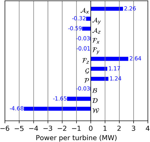
FIGURE 7. Energy budgets in the wind farm control volume Ω_wf. The budget terms are: advection of KE through the left/right $({\mathcal{A}}_x)$, south/north $({\mathcal{A}}_y)$ and bottom/top $({\mathcal{A}}_z)$ boundaries, turbulent fluxes through the left/right $({\mathcal{F}}_x)$, south/north $({\mathcal{F}}_y)$ and bottom/top $({\mathcal{F}}_z)$ boundaries, geostrophic forcing $(\mathcal{G})$, perturbation pressure gradients $(\mathcal{P})$, dissipation $(\mathcal{D})$ and energy extraction by wind turbines $(\mathcal{W})$.

The largest source of KE is the vertical turbulent flux of KE $({\mathcal{F}}_z=2.64\mathrm{M}\mathrm{W})$, contributing with 42% to the total energy sink. The fluxes through the lateral boundaries ${\mathcal{F}}_x$ and ${\mathcal{F}}_y$ are 2 orders of magnitude smaller than ${\mathcal{F}}_z$. The reason is that the surface area of the lateral boundaries is two orders of magnitude smaller than the surface area of the top or bottom boundary (Γ_x ≈ Γ_y ≈ 11 km² and Γ_z ≈ 2000 km²). Thus, turbulent fluxes through the left/right and south/north boundaries of the wind farm are negligible for the wind farm energy budget.

The energy input by the geostrophic forcing $\mathcal{G}$ and the mean perturbation pressure gradient $\mathcal{P}$ contribute with 1.17 MW and 1.24 MW, respectively. This corresponds to 18% and 20%, respectively, of the total energy sink. Consequently, $\mathcal{A}$, $\mathcal{G}$ and $\mathcal{P}$ have approximately the same magnitude $(\approx 20\%)$. The energy input by buoyancy forces is negligible small $(\mathcal{B}=-0.03\mathrm{M}\mathrm{W})$. This is an expected result for a neutrally stratified boundary layer.

3.3.2 Wind turbine energy budgets

The energy budgets for each wind turbine CV Ω_wt are shown in Figure 8. Due to the large spread of values it is difficult to derive quantitative statements from this Figure. However, the Figure shows the qualitative variation along the two dimensions of the wind farm. In general, there is a greater variation along the x-direction than along the y-direction. The variation along the x-direction is discussed in more detail in the next section. Variations along the y-direction occur, e.g., for ${\mathcal{A}}_x$, which is greater at the northwestern and southwestern wind farm corners. This correlates with $\mathcal{W}$, i.e., greater wind turbine powers also occur at these wind farm corners. The reason is the variation in the wind direction inside the wind farm: In the central, western part of the wind farm the wind direction is parallel to the turbine rows and thus the turbines in the third turbine column are in the full wake of the first turbine column (remember the staggered configuration). At the wind farm corners the wind direction is different (see Figure 3A) and thus the turbines are not in a full wake. This results in a higher turbine power but also in a larger difference between incoming and outgoing advection of KE and thus a greater ${\mathcal{A}}_x$. There is also a correlation between the vertical turbulent fluxes and the wind turbine power, i.e., greater wind turbine powers occur where the fluxes are greater. The energy input by the perturbation pressure gradient $\mathcal{P}$ is greatest at the southeastern wind farm corner, where also the largest pressure gradients occur (see Figure 3B). The energy input by the geostrophic forcing is approximately constant in the entire wind farm.

FIGURE 8

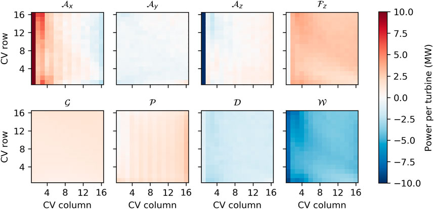
FIGURE 8. Energy budgets inside the wind turbine control volumes (CVs) Ω_wt. The budget terms are: advection of KE through left/right $({\mathcal{A}}_x)$, south/north $({\mathcal{A}}_y)$ and bottom/top $({\mathcal{A}}_z)$ boundaries, turbulent fluxes through bottom/top boundaries $({\mathcal{F}}_z)$, geostrophic forcing $(\mathcal{G})$, perturbation pressure gradients $(\mathcal{P})$, dissipation $(\mathcal{D})$ and energy extraction by wind turbines $(\mathcal{W})$. The buoyancy term $(\mathcal{B})$ and the horizontal turbulent fluxes (${\mathcal{F}}_x$ and ${\mathcal{F}}_y$) are not shown, because they are very small (see Figure 7). The values of ${\mathcal{A}}_x$ and ${\mathcal{A}}_z$ in the first CV column are larger than the color scale range, see Figure 9.

3.3.3 Wind turbine energy budgets averaged by column

To obtain more quantitative statements about the energy budgets inside the wind farm, Figure 9 shows the wind turbine CV energy budgets averaged by column. The terms $\mathcal{B}$ (buoyancy forces) and ${\mathcal{F}}_y$ (turbulent fluxes at the south/north boundaries) are not shown, because they are smaller than 0.05 MW in every column. In general, the budget terms show the same development as in the semi-infinite wind farm case presented in Maas (2022b).

FIGURE 9

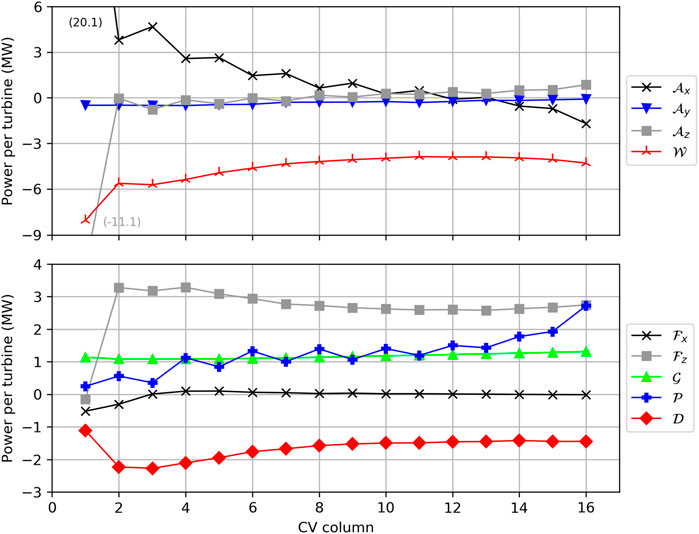
FIGURE 9. Energy budgets inside the wind turbine control volumes Ω_wt, averaged along y. The budget terms are: advection of KE through left/right $({\mathcal{A}}_x)$, south/north $({\mathcal{A}}_y)$ and bottom/top $({\mathcal{A}}_z)$ boundaries, energy extraction by wind turbines $(\mathcal{W})$, turbulent fluxes through bottom/top boundaries $({\mathcal{F}}_z)$, geostrophic forcing $(\mathcal{G})$, perturbation pressure gradients $(\mathcal{P})$ and dissipation $(\mathcal{D})$. The buoyancy term $(\mathcal{B})$ and the horizontal turbulent fluxes (${\mathcal{F}}_x$ and ${\mathcal{F}}_y$) are not shown, because they are very small (see Figure 7).

The advection of KE through the left/right boundaries (Figure 9A) is very large in the first CV (20.1 MW) and becomes negative (−1.7 MW) in the last CV. The flow accelerates in the last CV and thus more KE leaves the CV than it enters, resulting in a net negative KE budget. The streamwise acceleration (divergence) is related to a vertical convergence and thus KE enters the CV through the top boundary $({\mathcal{A}}_z=+0.85\mathrm{M}\mathrm{W})$. The opposite is the case in the first CV, where KE leaves the top boundary due to an ascending motion $({\mathcal{A}}_z=-11.1\mathrm{M}\mathrm{W})$. The evolution of ${\mathcal{A}}_x$ and ${\mathcal{A}}_z$ shows the same behavior as in semi-infinite wind farms (Allaerts and Meyers, 2017; Maas, 2022b). The advection of KE through the south/north boundaries of the CVs is ${\mathcal{A}}_y=-0.5\mathrm{M}\mathrm{W}$ at the first CV and decays to ${\mathcal{A}}_y=-0.1\mathrm{M}\mathrm{W}$ at the last CV. Thus, ${\mathcal{A}}_y$ is not zero as it is for a semi-infinite wind farm like in Allaerts and Meyers (2017) or Maas (2022b), but it has a much smaller magnitude than ${\mathcal{A}}_x$. Note that ${\mathcal{A}}_y$ is negative throughout the entire wind farm, indicating that the flow diverges in the y-direction up to the end of the wind farm and that the flow convergence is only present in the wake (see Figure 3). The development of $\mathcal{W}$ is discussed in Section 3.4.2.

The turbulent fluxes through the left/right boundaries (Figure 9B) are a small sink in the first two CVs $({\mathcal{F}}_x=-0.5\mathrm{M}\mathrm{W})$, because the outgoing flow contains more TKE than the incoming flow. For the rest of the wind farm ${\mathcal{F}}_x$ is approximately zero. The vertical turbulent fluxes are slightly negative in the first CV and reach their maximum value of ${\mathcal{F}}_z=3.3\mathrm{M}\mathrm{W}$ in CV 2 and then decay to ${\mathcal{F}}_z=2.6\mathrm{M}\mathrm{W}$ in CV 12.

The energy input by the geostrophic forcing $\mathcal{G}$ increases from 1.1 MW at CV 1–1.3 MW at CV 16. This increase is caused by the counterclockwise wind direction change along x resulting in a larger ageostrophic wind speed component and thus a larger energy input by the geostrophic forcing, as already described by Maas (2022b).

The energy input by the perturbation pressure gradients $\mathcal{P}$ increases from 0.2 MW at CV 1–2.7 MW at CV 16. The large value of $\mathcal{P}$ at the last CV causes the flow to accelerate, causing ${\mathcal{A}}_x$ to decrease and the turbine power $\mathcal{W}$ to increase in magnitude towards the end of the wind farm. Note that $\mathcal{P}$ shows oscillations with a wavelength of 2 CVs corresponding to 4 turbine spacings (4s_x = 5.76 km). These oscillations are related to small scale gravity waves that are triggered at the wind farm leading and trailing edge as described by Maas (2022b). These gravity waves have a wavelength of approximately 5.3 km and induce pressure oscillations in the boundary layer. The small scale gravity waves are not visible in Figure 5 because their pressure amplitude is much smaller than that of the visible large scale gravity waves.

The dissipation by the SGS model $(\mathcal{D})$ has the largest magnitude in CV 2 and 3. This is the location where also the largest TI occurs (see Figure 3C).

3.4 Power output and comparison with analytical wake models

3.4.1 Description of the analytical wake models

In the next section the wind turbine power output of PALM is discussed and compared with two analytical wake models, which are described in this section shortly. The two wake models are the NP model (Niayifar and Porté-Agel, 2016) and the Turbulence Optimized Park (TurbOPark) model (Pedersen et al., 2022). These wake models are chosen because they have a Gaussian velocity deficit profile in the wake and because their wake expansion rate depends on the local TI. The Gaussian profile represents the velocity deficit in the wake much more accurately than, e.g., a top-hat profile, as comparisons with LES data and wind tunnel measurements have shown (Bastankhah and Porté-Agel, 2014). Accounting for the local TI, i.e., the sum of the ambient TI and the turbine generated TI, results in a more realistic wake expansion rate than accounting for only the ambient TI (Lissaman, 1979; Nygaard et al., 2022). Both wake models are based on the momentum-conserving velocity deficit model for a single turbine wake proposed by Bastankhah and Porté-Agel (2014). For each wind turbine there is an image wind turbine mirrored at z = 0 to account for the effect of the ground. The wake models differ in the wake superposition principle and the turbulence model.

In the NP model the superposition of wakes is performed by a linear sum of the velocity deficits, which conserves the momentum (Lissaman, 1979; Bastankhah and Porté-Agel, 2014). The turbine generated turbulence is modeled according to Crespo and Herna´ndez (1996). Note that this model is only valid for streamwise TIs between 7% and 14% and that the first 2 turbine columns are exposed to the ambient streamwise TI, which is only 4.3%. For a given location only the TI caused by the nearest upstream turbine is considered and no superposition is performed (Bastankhah and Porté-Agel, 2014, p. 5).

In the TurbOPark model the superposition of wakes is performed by a quadratic sum of the velocity deficits, which conserves the kinetic energy (Katic et al., 1987; Nygaard et al., 2022). The turbine generated turbulence is modeled according to Frandsen (2007). The superposition of the ambient TI with the turbine generated TI of all wakes at a given location is performed by a quadratic sum, which is a TKE- or variance-conserving method.

The computations for the wake models are performed with the open source wind farm simulation tool PyWake (Pedersen et al., 2019). Meteorological input parameters are the mean hub height wind speed (9 m ·s⁻¹), the wind shear exponent (0.088), the ambient streamwise TI at hub height (4.3%) and the wind direction (270°). Wind turbine specific input parameters are the rotor diameter, the hub height, the coordinates of the wind turbines and the thrust and power coefficients at different wind speeds, that are available at the data repository given in Gaertner et al. (2020).

3.4.2 Results of the wake model comparison

The electrical wind turbine power output of PALM and the two wake models is shown in Figure 10. There are large differences in the qualitative distribution of the turbine power between PALM and the wake models. For the TurbOPark model, the turbine power only varies along the turbine rows and is constant inside a turbine column. For the NP model the turbine power is larger at the southern and northern wind farm boundaries than inside the wind farm. This effect is largest for the most downstream located turbines and is caused by the linear superposition method for the velocity deficit but also by the different turbulence model used in the NP model. However, the largest variation inside a turbine column is present in PALM. In the first column, the highest turbine power occurs at the most northern and southern turbines, because the blockage effect (or pressure) is smallest there (see Figure 3B). But also for further downstream located columns the power variation is very large, e.g., 3.8 MW–6.2 MW in column 3. This large variation is caused by the spatial variation of the wind direction inside the wind farm that results in a full-wake situation for a row-parallel flow and to a partial or no-wake situation for other wind directions (see Figure 3A). Consequently the smallest turbine power occurs at row 1, column 23, where the wind direction is parallel to the turbine rows.

FIGURE 10

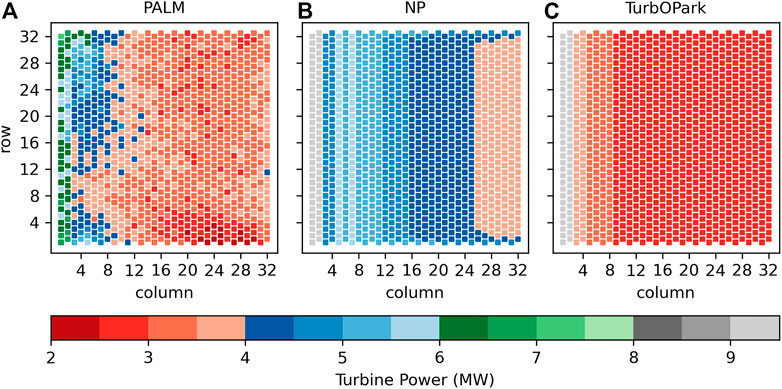
FIGURE 10. Wind turbine power of the LES model PALM (A), the Niayifar and Porté-Agel model (B) and the TurbOPark model (C). For PALM, the power is averaged over the last 4 h of the main simulation.

Because a quantitative comparison between the models is difficult with the color diagram shown in Figure 10, the column-wise averaged wind turbine power is shown in Figure 11. The figure shows the results of two different PyWake simulations. In Figure 11A the hub height wind speed is set to the hub height inflow wind speed in PALM (v₁ = 9.00 m·s⁻¹). In Figure 11B the hub height wind speed is set to the wind speed 2.5 D upstream of the first turbine column averaged along the wind farm width in PALM (v₂ = 7.94 m·s⁻¹) to account for the global blockage effect.

FIGURE 11

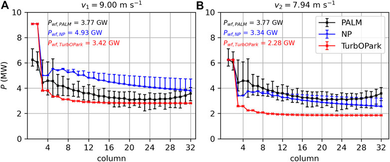
FIGURE 11. Wind turbine power of the LES model PALM, the Niayifar and Porté-Agel model (NP) and the TurbOPark model. The markers represent the column-wise averaged power and the error bars represent the maximal and minimal power in the respective wind farm column. In (A) the reference wind speed for the wake models is set to the inflow wind speed at hub height of the LES (9.00 m ·s⁻¹). In the (B) the reference wind speed is reduced to 7.94 m ·s⁻¹, which is the wind speed 2.5 D upstream of the first column averaged along the wind farm width in PALM. The total wind farm powers (P_wf) are also given.

In PALM, the mean turbine power in the first column is 6.2 MW. This is 32% less than the power of the IEA 15 MW reference wind turbine at a hub height wind speed of 9.0 m·s⁻¹ (9.1 MW). The reason is the global blockage effect, that reduces the mean hub height wind speed in the first column by approximately 1 m·s⁻¹. In column 3 and 4 the mean turbine power has dropped to approximately 4.5 MW, because most of the turbines are in the wake of a turbine in column 1 or 2. Some turbines, however, are not in a full wake, as discussed above and thus there is a large spread between the minimum and maximum turbine power in these columns. Further downstream, the power drops further due to a decrease in the horizontal advection of KE ${\mathcal{A}}_x$ and a decrease in the vertical turbulent fluxes ${\mathcal{F}}_z$ (see Figure 9). At column 20 the mean turbine power has reached a minimum of 3.1 MW. Further downstream the mean turbine power increases to 3.6 MW at the last column. This increase in power is caused by an increase in the energy input by the pressure gradient $\mathcal{P}$ (see Figure 9). The total wind farm power is P_wf,PALM = 3.77 GW, resulting in a wind farm efficiency of:

${\eta }_{wf,PALM}=\frac{P_{wf,PALM}}{N_{wt}{P}_{\mathit{ref}}}=\frac{3.77\mathrm{G}\mathrm{W}}{1024\times 9.1\mathrm{M}\mathrm{W}}=40.5\%.(13)$

In Figure 11A the mean turbine power in the first two columns of the NP and TurbOPark model is 9.1 MW, which is the power of the IEA 15 MW reference wind turbine at a hub height wind speed of 9.0 m ·s⁻¹. This is 47% more than in PALM because the NP and TurbOPark model do not account for the global blockage effect. In PyWake it is possible to account for the local blockage effect, i.e., the flow deceleration upstream of each rotor disc. However, using this local blockage model affects the wind farm power by less than 0.5%. Thus, the magnitude of the global blockage effect is approximately two orders of magnitude greater than the sum of the local blockage effects of all wind turbines. Similar results have also been reported by Centurelli et al. (2021).

In Figure 11B, where the hub height wind speed for the wake models is reduced to v₂ = 7.94 m ·s⁻¹, the turbine power in the first column of the wake models agrees with that of PALM. Thus, the following discussion is based on Figure 11B.

For the NP model the turbine power drops to 3.4 MW in column 3 and 4 and then increases to 3.7 MW in column 7 due to the increases TI generated by the upstream turbines. From there on the turbine power decreases monotonically up to the end of the wind farm, where it reaches 2.6 MW. In the bulk of the wind farm the NP model underestimates the turbine power by only 7%. Larger differences of up to −28% occur towards the end of the wind farm. The total wind farm power output is P_wf,NP = 3.34 GW, which is 11% less than that of PALM and corresponds to a wind farm efficiency of η_wf,NP = 35.8%.

For the TurbOPark model the turbine power drops to 2.6 MW in column 3 and 4. Due to the quadratic superposition of the velocity deficits, the turbine power reaches an equilibrium value of 1.9 MW at approximately column 16. This results in deviations of up to −51% relative to PALM in column 5. The total wind farm power output is P_wf,TurbOPark = 2.28 GW, which is 40% less than that of PALM and corresponds to a wind farm efficiency of η_wf,TurbOPark = 24.5%.

What are the reasons for these large discrepancies between the results of the LES and the wake models? As described in the previous section, the wake models are momentum-conserving (or energy-conserving in case of the wake superposition in the TurbOPark model). That means that there are no momentum or energy sinks except the wind turbines itself. There are also no momentum or energy sources except the advection of KE into the wind farm. But, as the energy budget analysis of the LES shows, there are KE sources and sinks that are at least equally important than the advection of KE. The sources are the energy input by the geostrophic forcing $(\mathcal{G})$ and by the perturbation pressure gradients $(\mathcal{P})$. The vertical turbulent fluxes $({\mathcal{F}}_z)$ are also an energy source but they are part of the wake expansion process of the wake models (expansion and speed recovery through turbulent mixing). There are also important energy sinks like the loss of KE through the northern and southern wind farm boundaries ${\mathcal{A}}_y$, the bottom and top wind farm boundaries $({\mathcal{A}}_z)$ and the loss of KE by dissipation $(\mathcal{D})$. Because the wake models do not consider these energy sources and sinks, the wake models overestimate or underestimate the total wind farm power, depending on which reference hub height wind speed is chosen.

The LES results show that, if all relevant physics are modeled, many complex flow effects occur in a wind farm of this size. These relevant physics are, e.g., the consideration of Coriolis, pressure and buoyancy forces resulting in flow effects like gravity waves, global blockage effect, flow deflection and flow acceleration. The complexity of the flow causes a large spread in the wind turbine power, as shown in Figure 10A. The investigated wake models neglect the above named physics. This seems to be a valid simplification for small wind farms in which the named flow effects do not occur. But for large, multi-gigawatt wind farms as in this study this simplification is not valid any more. The analytical wake models thus underestimate the variation of the turbine power inside the turbine columns and underestimate the total wind farm power by up to 40%.

Improvements could be achieved by taking some of the neglected physics into account. The largest deviations occur at the first and last turbine column and are caused by the neglection of the perturbation pressure distribution. The perturbation pressure distribution is responsible for the global blockage effect and the flow acceleration at the end of the wind farm. Thus, taking these effects into account will probably significantly improve the large wind farm power prediction capability of the investigated wake models. Two tasks have to be solved to include these effects in to the wake models: First, modeling of the gravity wave induced pressure distribution in the wind farm. Second, modeling the effect of this pressure distribution on the velocity field, e.g., by applying Bernoulli’s principle. Information for modeling gravity wave induced pressure gradients in wind farms is provided by Smith (2009), Allaerts et al. (2018), Allaerts and Meyers (2019), Lanzilao and Meyers (2021) and Devesse et al. (2022). A wake model that considers the effect of streamwise pressure gradients was recently proposed by Dar and Porté-Agel (2022). It is designed for topography induced pressure gradients but it might also be suitable for gravity wave induced pressure gradients. Unfortunately, this model is not part of PyWake and could not be tested in this study.

4 Discussion

In this study the results of an LES of a 15 GW wind farm are presented and compared with analytical wake models. One aim of this study is to investigate differences between the flow field of the finite-size wind farm setup as used in this study with a semi-infinite wind farm setup as used in the study of Maas (2022b). The results show that the finite-size wind farm setup causes an even more complex flow than the semi-infinite wind farm setup. Additional effects are the crosswise flow divergence in the wind farm and the crosswise flow convergence in the wind farm wake. The semi-infinite wind farm setup of Maas (2022b) generates supergeostrophic wind speeds in the wake, which do not occur for the finite-size wind farm in this study. Thus, it can be concluded that using a semi-infinite wind farm setup for multi-gigawatt wind farms suppresses or amplifies important flow features that occur in the more realistic finite-size wind farm setup.

The energy budget analysis shows that there is an additional loss of KE through the southern and northern wind farm boundaries that do not exist for a semi-infinite wind farm setup. However, this additional loss is compensated by a reduction of the KE loss by advection through the bottom and top wind farm boundaries. The turbulent flux of KE through all lateral wind farm boundaries is two orders of magnitude smaller than the turbulent fluxes through the bottom and top wind farm boundaries and can thus be neglected.

The second aim of this study is to compare the wind turbine power output of the LES model PALM with two analytical wake models: The NP model (Niayifar and Porté-Agel, 2016) and the TurbOPark model (Pedersen et al., 2022). The comparison shows that there are large discrepancies between the wind farm power predicted by the wake models and by PALM. In the first turbine column the wake models overestimate the power by 47%, because they do not account for the global blockage effect. If the reference hub height wind speed of the wake models is reduced to account for the global blockage effect, then they underestimate the wind farm power by 11% and 40% for the NP and TurbOPark model, respectively. Due to the spatial variability of the wind direction in PALM, there is a large variation in the turbine power throughout the wind farm. This variability is not present in the wake models.

The large discrepancies between the results of PALM and the wake models occur because the wake models neglect most of the relevant physical processes. This has two consequences: First, the flow field do not feature the flow complexity, e.g., the wind direction variability, that the results of the LES reveal. Second, important energy sources and sinks, such as the energy input by the geostrophic forcing or the perturbation pressure gradients, are neglected. This seems to be a valid simplification for small wind farms in which the named flow effects do not occur and the largest energy source is the advection of KE. But for large, multi-gigawatt wind farms as in this study this simplification is not valid any more, because other energy sources and sinks become relevant. Improvements could be achieved by taking some of the neglected physics, especially the pressure distribution, into account.

The LES results provide interesting and valuable insights into the flow of potential large offshore wind farms. It should be noted, however, that the results are based on a very idealized simulation setup that might deviate from reality significantly. For example, stationarity, barotropic conditions, a constant wind and temperature stratification profile in the free atmosphere and a homogeneous surface are assumed. A deviation from these idealized conditions might weaken or strengthen the described flow effects. The wind farm blocks 1/3 of the domain width, so that the magnitude of the pressure gradients and the wake deflection might still be overestimated. Additionally, only one meteorological and wind farm setup is investigated. A different boundary layer height, stability, surface roughness or turbine arrangement may change the results. Further research is needed to quantify the effect of the named variations.

Data availability statement

The datasets presented in this study can be found in online repositories. The names of the repository/repositories and accession number(s) can be found below: https://doi.org/10.25835/39jgn8ac Research Data Repository of the Leibniz University Hannover.

Author contributions

The author confirms being the sole contributor of this work and has approved it for publication.

Funding

This work was funded by the Federal Maritime and Hydrographic Agency (BSH, Grant No. 10044580) and supported by the North German Supercomputing Alliance (HLRN).

Acknowledgments

I thank my supervisor Siegfried Raasch for guiding the manuscript preparation.

Conflict of interest

The author declares that the research was conducted in the absence of any commercial or financial relationships that could be construed as a potential conflict of interest.

Publisher’s note

All claims expressed in this article are solely those of the authors and do not necessarily represent those of their affiliated organizations, or those of the publisher, the editors and the reviewers. Any product that may be evaluated in this article, or claim that may be made by its manufacturer, is not guaranteed or endorsed by the publisher.

References

Allaerts, D., and Meyers, J. (2017). Boundary-layer development and gravity waves in conventionally neutral wind farms. J. Fluid Mech. 814, 95–130. doi:10.1017/jfm.2017.11

CrossRef Full Text | Google Scholar

Allaerts, D., and Meyers, J. (2019). Sensitivity and feedback of wind-farm-induced gravity waves. J. Fluid Mech. 862, 990–1028. doi:10.1017/jfm.2018.969

PubMed Abstract | CrossRef Full Text | Google Scholar

Allaerts, D., Broucke, S. V., van Lipzig, N., and Meyers, J. (2018). Annual impact of wind-farm gravity waves on the Belgian-Dutch offshore wind-farm cluster. J. Phys. Conf. Ser. 1037, 072006. doi:10.1088/1742-6596/1037/7/072006

CrossRef Full Text | Google Scholar

Bastankhah, M., and Porté-Agel, F. (2014). A new analytical model for wind-turbine wakes. Renew. Energy 70, 116–123. doi:10.1016/j.renene.2014.01.002

CrossRef Full Text | Google Scholar

BSH (2022). Entwurf flächenentwicklungsplan. Tech. rep. Hamburg: Bundesamt für Seeshifffahrt und Hydrographie.

Google Scholar

Centurelli, G., Vollmer, L., Schmidt, J., Dörenk mper, M., Schröder, M., Lukassen, L. J., et al. (2021). Evaluating global blockage engineering parametrizations with LES. J. Phys. Conf. Ser. 1934, 012021. doi:10.1088/1742-6596/1934/1/012021

CrossRef Full Text | Google Scholar

Crespo, A., and Herna´ndez, J. (1996). Turbulence characteristics in wind-turbine wakes. J. Wind Eng. Indust. Aerodyn. 61, 71–85. doi:10.1016/0167-6105(95)00033-X

CrossRef Full Text | Google Scholar

Dar, A. S., and Porté-Agel, F. (2022). An analytical model for wind turbine wakes under pressure gradient. Energies 15, 5345. doi:10.3390/en15155345

CrossRef Full Text | Google Scholar

Deardorff, J. W. (1980). Stratocumulus-capped mixed layers derived from a three-dimensional model. Boundary-Layer Meteorol. 18, 495–527. doi:10.1007/BF00119502

CrossRef Full Text | Google Scholar

Devesse, K., Lanzilao, L., Jamaer, S., Van Lipzig, N., and Meyers, J. (2022). Including realistic upper atmospheres in a wind-farm gravity-wave model. Wind Energy Sci. 7, 1367–1382. doi:10.5194/wes-7-1367-2022

CrossRef Full Text | Google Scholar

Dörenkämper, M., Witha, B., Steinfeld, G., Heinemann, D., and Kühn, M. (2015). The impact of stable atmospheric boundary layers on wind-turbine wakes within offshore wind farms. J. Wind Eng. Indust. Aerodyn. 144, 146–153. doi:10.1016/j.jweia.2014.12.011

CrossRef Full Text | Google Scholar

Frandsen, S. T. (2007). Turbulence and turbulence-generated structural loading in wind turbine clusters. Ph.D. thesis. Technical University of Denmark.

Google Scholar

Frederiksen, M., de Croo, A., Rutte, M., and Scholz, O. (2022). The esbjerg declaration. Tech. rep. The Federal Ministry for Economic Affairs and Climate Action of Germany.

Google Scholar

Gaertner, E., Rinker, J., Sethuraman, L., Zahle, F., Anderson, B., Barter, G., et al. (2020). Definition of the IEA wind 15-megawatt offshore reference wind turbine. Tech. rep. Golden, CO: National Renewable Energy Laboratory.

Google Scholar

Katic, I., Højstrup, J., and Jensen, N. (1987). A simple model for cluster efficiency. Eur. wind energy Assoc. Conf. Exhib. 1, 407–410.

Google Scholar

Klemp, J. B., and Lilly, D. K. (1978). Numerical simulation of hydrostatic mountain waves. J. Atmos. Sci. 35, 78–107. doi:10.1175/1520-0469(1978)035<0078:NSOHMW>2.0.CO;2

CrossRef Full Text | Google Scholar

Krüger, S., Steinfeld, G., Kraft, M., and Lukassen, L. J. (2022). Validation of a coupled atmospheric-aeroelastic model system for wind turbine power and load calculations. Wind Energy Sci. 7, 323–344. doi:10.5194/wes-7-323-2022

CrossRef Full Text | Google Scholar

Lanzilao, L., and Meyers, J. (2021). Set-point optimization in wind farms to mitigate effects of flow blockage induced by atmospheric gravity waves. Wind Energy Sci. 6, 247–271. doi:10.5194/wes-6-247-2021

CrossRef Full Text | Google Scholar

Lanzilao, L., and Meyers, J. (2022). Effects of self-induced gravity waves on finite wind-farm operations using a large-eddy simulation framework. J. Phys. Conf. Ser. 2265, 022043. doi:10.1088/1742-6596/2265/2/022043

CrossRef Full Text | Google Scholar

Lissaman, P. B. (1979). Energy effectiveness of arbitrary arrays of wind turbines. J. energy 3, 323–328. doi:10.2514/3.62441

CrossRef Full Text | Google Scholar

Maas, O., and Raasch, S. (2022). Wake properties and power output of very large wind farms for different meteorological conditions and turbine spacings: A large-eddy simulation case study for the German Bight. Wind Energy Sci. 7, 715–739. doi:10.5194/wes-7-715-2022

CrossRef Full Text | Google Scholar

Maas, O. (2022a). LES of a 15 GW wind farm. [Dataset]. doi:10.25835/39jgn8ac

CrossRef Full Text | Google Scholar

Maas, O. (2022b). Preprint: From gigawatt to multi-gigawatt wind farms: Wake effects, energy budgets and inertial gravity waves investigated by large-eddy simulations. Wind Energy Sci. Discuss. 2022, 1–31. doi:10.5194/wes-2022-63

CrossRef Full Text | Google Scholar

Maronga, B., Moene, A. F., van Dinther, D., Raasch, S., Bosveld, F. C., and Gioli, B. (2013). Derivation of structure parameters of temperature and humidity in the convective boundary layer from large-eddy simulations and implications for the interpretation of scintillometer observations. Boundary-Layer Meteorol. 148, 1–30. doi:10.1007/s10546-013-9801-6

CrossRef Full Text | Google Scholar

Maronga, B., Banzhaf, S., Burmeister, C., Esch, T., Forkel, R., Fröhlich, D., et al. (2020). Overview of the PALM model system 6.0. Geosci. Model Dev. 13, 1335–1372. doi:10.5194/gmd-13-1335-2020

CrossRef Full Text | Google Scholar

Miller, M. J., and Thorpe, A. J. (1981). Radiation conditions for the lateral boundaries of limited-area numerical models. Q. J. R. Meteorol. Soc. 107, 615–628. doi:10.1002/qj.49710745310

CrossRef Full Text | Google Scholar

Moeng, C.-H., and Wyngaard, J. C. (1988). Spectral analysis of large-eddy simulations of the convective boundary layer. J. Atmos. Sci. 45, 3573–3587. doi:10.1175/1520-0469(1988)045<3573:SAOLES>2.0.CO;2

CrossRef Full Text | Google Scholar

Munters, W., Meneveau, C., and Meyers, J. (2016). Shifted periodic boundary conditions for simulations of wall-bounded turbulent flows. Phys. Fluids 28, 025112. doi:10.1063/1.4941912

CrossRef Full Text | Google Scholar

Niayifar, A., and Porté-Agel, F. (2016). Analytical modeling of wind farms: A new approach for power prediction. Energies 9, 741–813. doi:10.3390/en9090741

CrossRef Full Text | Google Scholar

Nygaard, N. G., Poulsen, L., Svensson, E., and Pedersen, J. G. (2022). Large-scale benchmarking of wake models for offshore wind farms. J. Phys. Conf. Ser. 2265, 022008. doi:10.1088/1742-6596/2265/2/022008

CrossRef Full Text | Google Scholar

Orlanski, I. (1976). A simple boundary condition for unbounded hyperbolic flows. J. Comput. Phys. 21, 251–269. doi:10.1016/0021-9991(76)90023-1

CrossRef Full Text | Google Scholar

Pedersen, M. M., van der Laan, P., Friis-Møller, M., Rinker, J., and Réthoré, P.-E. (2019). DTUWindEnergy/PyWake: PyWake. [Dataset]. doi:10.5281/zenodo.2562662

CrossRef Full Text | Google Scholar

Pedersen, J. G., Svensson, E., Poulsen, L., and Nygaard, N. G. (2022). Turbulence Optimized Park model with Gaussian wake profile. J. Phys. Conf. Ser. 2265, 022063. doi:10.1088/1742-6596/2265/2/022063

CrossRef Full Text | Google Scholar

Porté-Agel, F., Bastankhah, M., and Shamsoddin, S. (2020). Wind-turbine and wind-farm flows: A review. Boundary-Layer Meteorol. 174, 1–59. doi:10.1007/s10546-019-00473-0

PubMed Abstract | CrossRef Full Text | Google Scholar

Saiki, E. M., Moeng, C.-H., and Sullivan, P. P. (2000). Large-eddy simulation of the stably stratified planetary boundary layer. Boundary-Layer Meteorol. 95, 1–30. doi:10.1023/A:1002428223156

CrossRef Full Text | Google Scholar

Smith, R. B. (2009). Gravity wave effects on wind farm efficiency. Wind Energy 13, 449–458. doi:10.1002/we.366

CrossRef Full Text | Google Scholar

Steinfeld, G., Witha, B., Dörenkämper, M., and Gryschka, M. (2015). Hochauflösende Large-Eddy-Simulationen zur Untersuchung der Strömungsverhältnisse in Offshore-Windparks. promet - Meteorol. Fortbild. 39, 163–180.

Google Scholar

Stevens, R. J., Gayme, D. F., and Meneveau, C. (2016). Effects of turbine spacing on the power output of extended wind-farms. Wind Energy 19, 359–370. doi:10.1002/we.1835

CrossRef Full Text | Google Scholar

Taylor, J. R., and Sarkar, S. (2007). Internal gravity waves generated by a turbulent bottom Ekman layer. J. Fluid Mech. 590, 331–354. doi:10.1017/S0022112007008087

CrossRef Full Text | Google Scholar

Wicker, L. J., and Skamarock, W. C. (2002). Time-splitting methods for elastic models using forward time schemes. Mon. Weather Rev. 130, 2088–2097. doi:10.1175/1520-0493(2002)130<2088:TSMFEM>2.0.CO;2

CrossRef Full Text | Google Scholar

Witha, B., Steinfeld, G., Dörenkämper, M., and Heinemann, D. (2014). Large-eddy simulation of multiple wakes in offshore wind farms. J. Phys. Conf. Ser. 555, 012108. doi:10.1088/1742-6596/555/1/012108

CrossRef Full Text | Google Scholar

Wu, Y.-T., and Porté-Agel, F. (2011). Large-eddy simulation of wind-turbine wakes: Evaluation of turbine parametrisations. Boundary-Layer Meteorol. 138, 345–366. doi:10.1007/s10546-010-9569-x

CrossRef Full Text | Google Scholar

Wu, K. L., and Porté-Agel, F. (2017). Flow adjustment inside and around large finite-size wind farms. Energies 10, 2164–2169. doi:10.3390/en10122164

CrossRef Full Text | Google Scholar

Zhang, M., Arendshorst, M. G., and Stevens, R. J. (2019). Large eddy simulations of the effect of vertical staggering in large wind farms. Wind Energy 22, 189–204. doi:10.1002/we.2278

CrossRef Full Text | Google Scholar