Data model-based toolpath generation techniques for CNC milling machines

1 Introduction

Toolpath generation is a core task in computer numerical control (CNC) milling machine operations, directly impacting processing quality, efficiency, and tool lifespan (Chen et al., 2021). As a research area with tremendous potential, toolpath generation technology has been extensively explored by scholars worldwide. Techniques such as real-time toolpath generation, toolpath generation for multi-axis and five-axis machine tools, and data-driven trajectory generation have been proposed (Li and Tang, 2021). While these techniques have met the requirements of CNC equipment in the past, they are increasingly unable to satisfy current mass demands due to technological innovations and rising structural requirements for processed parts (Huang et al., 2020). With the rise of three-dimensional (3D) data models, point cloud models, as a special type of 3D model, are widely used in various fields due to their high resolution, precise 3D representation, and real-time data characteristics, addressing complex issues (Praveen et al., 2020). In light of this, the research innovatively introduces point cloud models based on 3D models. After preprocessing, including denoising and down-sampling, new technical methods for toolpath generation in rough and finish machining are proposed, aiming to advance the application of data models in toolpath generation technology for CNC milling machines. This research is divided into four parts: the first analyzes and summarizes previous research, the second introduces how novel toolpath generation methods for rough and finish machining are designed using point cloud data models, the third tests the performance of these two methods, and the final part provides a summary of the article.

2 Related work

CNC milling machines are commonly used in modern manufacturing to precisely and efficiently process various complex curved components. The generation of toolpath trajectories is a critical step in the machining process of NC milling machines, directly impacting the quality and efficiency of part manufacturing. Traditional methods for generating toolpath trajectories are primarily based on experience and expert knowledge, leading to challenges in design and difficulty in controlling the outcomes. In response to these challenges, researchers both domestically and internationally have conducted various studies. Li and collaborators identified issues in the side milling of thin-walled workpieces, where excessive cutting forces or directional deviations could compromise the geometric accuracy of the processed parts. In addressing this, the research team proposed a method for generating multi-pass toolpaths using semi-finish machining with double-sided milling. Experimental results demonstrated that this approach is more favorable for the finish machining of thin-walled workpieces compared to traditional milling methods, exhibiting robustness (Li et al., 2021). He and his colleagues observed that discontinuities in the tangential components of toolpath trajectories in five-axis hybrid numerical control machines could result in speed fluctuations, adversely affecting the surface quality of the workpiece. To mitigate this issue, the research team introduced a smooth toolpath interpolation method. Experimental results indicated that this method is highly effective in practical machining trials, ensuring continuity in cutting parameters (He et al., 2022). Liu and his co-authors aimed to enhance curvature continuity and smoothness during the cutting process. They proposed a multi-relationship spiral trochoidal milling strategy by combining toolpath trajectories and tool axis vectors in five-axis side milling. Experimental results demonstrated the strong practical feasibility of this method, contributing to improved part manufacturing quality (Liu et al., 2020). Liang and collaborators sought to enhance the machining effectiveness of non-uniform rational B-spline surfaces in computer-aided design and manufacturing. The research team proposed a universal method for generating toolpath trajectories for such surfaces. Experimental results showed that this method is applicable to various non-uniform rational B-spline surfaces, offering higher smoothness and shorter toolpath lengths (Liang et al., 2020).

The CNC milling machine toolpath generation technology can use various data models to describe the characteristics and patterns of toolpaths. Commonly used models include B-spline curve models, simulation models, 3D models, and machine learning models. To enhance the global optimization effect of polynomial functions, Gawali and others introduced the B-spline consistency algorithm for improvement and proposed a polynomial B-spline optimization algorithm. Experimental results demonstrate that this algorithm consistently captures global minima with specified precision compared to CENSO evaluation and GloptiPoly solution methods (Gawali et al., 2021). Liu and others aimed to model and analyze the reliability of machine tool spindles, quantifying uncertainty factors using imprecise probability theory. They proposed a reliability modeling and analysis method based on imprecise probability theory. Simulation results show that this method is applicable to various uncertain factors and data, demonstrating strong suitability for analyzing machine tool spindles (Liu et al., 2022). Sheng and others identified issues with long production cycles and low efficiency when using artificial data measurements for computer-aided design. Consequently, they proposed a control system for flat processing machine tools using machine vision. Experimental results indicate that this system significantly improves production efficiency and reduces errors in image contouring (Sheng et al., 2022). Sales and his colleagues observed that topology optimization, especially in path planning during computer-aided design, is often overlooked, leading to a loss of structural performance in the designed material. They proposed a toolpath generation strategy based on straight-line topology optimization. Experimental results suggest that this method has certain advantages when applied to computer-aided manufacturing, significantly improving structural stiffness (Sales et al., 2021).

In summary, CNC milling machine toolpath generation technology has significantly improved, and the use of data models for toolpath generation has been confirmed. However, challenges remain in handling large-scale data and real-time processing during the manufacturing process. To address this, researchers are exploring the use of point cloud models in 3D models for data analysis, aiming to construct a novel CNC milling machine toolpath generation system to enhance processing efficiency and quality.

3 CNC milling machine toolpath generation based on point cloud models

For different point cloud data models, the research initially focuses on denoising and down-sampling point cloud models, providing an effective data foundation for subsequent toolpath generation methods. Building upon this foundation, the study explores improvements in traditional toolpath generation techniques, specifically investigating methods for toolpath generation in rough machining and finish machining.

3.1 Denoising and downsampling of point cloud models

Point cloud models are a type of geometric model used to represent discrete points in 3D space. Each point in the model contains 3D coordinates and RGB values (Nirala and Agrawal, 2020). These models can be classified into scattered point clouds, array point clouds, and scanned point clouds. The points of the scanned point cloud all lie on the scan line, which is not fully present. The tracing line is not fully present means that the scanning process, the scanning line (or scanning path) does not completely cover or pass through the entire surface of the workpiece, or there are some missed parts. This may be due to the limitations of the scanning equipment, obstruction during the scanning process, scanning angle or positional problems, and so on. Array point cloud data is uniformly distributed with points at each intersection. Scattered point clouds, on the other hand, exhibit a completely random distribution. Regardless of the type of point cloud, during actual instrument measurements, the data are susceptible to noise and outliers due to the inherent characteristics of the measurement system and its precision. Therefore, in order to avoid data errors on the subsequent path generation, the acquisition and noise reduction processing of the point cloud data is particularly important. First, the study uses a high-performance 3D scanning equipment to scan the data. The process ensures a sufficiently high sampling density to capture the minute details of the workpiece surface. In addition, the sampling spacing was set to a fixed value, which ensured that the point cloud data were adequately captured. By using this scanning equipment, the study obtained accurate and detailed point cloud data models, which provided a reliable basis for subsequent algorithmic studies. Common denoising methods include radius filtering, Gaussian filtering, interactive denoising and the four-point denoising method (He et al., 2021). While removing noise, the four-point noise reduction method is more capable of retaining the detail information in the point cloud data compared to radius filtering and Gaussian filtering, and at the same time realizes a better smoothing effect, which makes the surface of the point cloud smoother without losing the key shape features (Zheng et al., 2022). Most importantly, the four-point noise reduction method has a certain degree of adaptivity, which can better adapt to the different densities and distributions in the point cloud (Leal et al., 2020). The four-point denoising method has been introduced in this study. The four-point denoising method uses a single scan line as a reference and calculates the spatial distances between consecutive points $P_{i,j}$, $P_{i,j+1}$, $P_{i,j-1}$, $P_{i,j+2}$. The distance calculation between any two points is given by Formula (Chen et al., 2021).

$dist=\sqrt{{\left(x_2-x_1\right)}^2+{\left(y_2-y_1\right)}^2+{\left(z_2-z_1\right)}^2}(1)$

In Formula 1 (Chen et al., 2021), $x_1,y_1,z_1$ represents the 3D spatial position of the first point, and $x_2,y_2,z_2$ represents the 3D spatial position of the second point. If points $P_{i,j}$ and $P_{i,j+1}$ are situated on the same side of the line connecting $P_{i,j-1}$ and $P_{i,j+2}$, the four-point judgment process is described in Formula (Li and Tang, 2021).

$\left\{\begin{array}{l}{d}_1-d_2>\epsilon ,P_{i,j}\\ d_1-d_2<\epsilon ,P_{i,j}\cup P_{i,j+1}\end{array}\right.(2)$

In Formula 2 (Li and Tang, 2021), $\epsilon$ is a given threshold, $i$ represents the $i$-th scan line, and $j$ represents a point on the scan line. The four-point denoising process is illustrated in Figure 1.

FIGURE 1

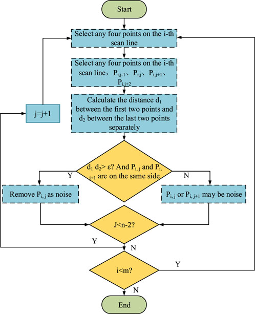
FIGURE 1. Four point noise reduction process.

From Figure 1, it can be observed that the process involves setting values for $i$ and $j$, selecting four points on the $i$-th scan line, and calculating the distances between pairs of points. If the difference in distances is greater than the threshold, point $P_{i,j}$ is identified as noise and removed. If the difference is less than the threshold, the noise point could be $P_{i,j}$ or $P_{i,j+1}$. In this case, a smoothing denoising operation is performed using the arithmetic mean of PL, $P_{i,j}$, and PI. If points $P_{i,j}$ and $P_{i,j+1}$ are on opposite sides of the line connecting $P_{i,j-1}$ and $P_{i,j+2}$, then $P_{i,j}$ is identified as noise and is removed, and the arithmetic mean of $P_{i,j-1}$ and $P_{i,j+1}$ is used for interpolation. This process is repeated until the number of points on the scan line is less than $n-2$, and the number of scan lines is less than $m$, at which point the results are outputted. After denoising, down-sampling of the point cloud data is necessary to reduce the computational load of the toolpath algorithm. The study employs an octree structure to perform 3D grid processing on the point cloud model. The octree structure is illustrated in Figure 2.

FIGURE 2

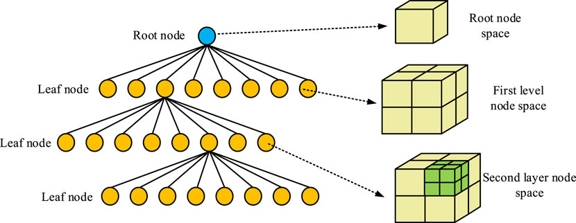
FIGURE 2. Schematic diagram of octree structure.

In Figure 2, each face of the cube is subdivided in a fixed format. There is one point for each node, representing a cubic model. This process is carried out for each face of the node cube, and eight initial child nodes are yielded. This process is repeated until the volume of the cubic network or the point cloud data is insufficient to support further subdivision, at which point the operation ceases. In the actual scanned point cloud, a bounding box of length and width is created and divided into KW grids. Grids with data points are considered real grids, while those without data points are virtual grids. The center points of real grids are used to replace other point cloud data in the scan line, and this process is repeated until all scan lines are processed.

3.2 Rough toolpath generation based on point cloud models

The toolpath refers to the trajectory of the tool’s movement relative to the workpiece in CNC machining. This process involves tool approach, machining, milling, and the path traveled back to the tool approach point. The toolpath comprises concepts such as tool position points, tool contact points, step size, pitch, and processing bandwidth (Choudhuri et al., 2023). General trajectory generation methods typically go through steps such as point cloud data modeling, surface data reconstruction, and surface path planning. Due to the time-consuming and labor-intensive nature of the reconstruction step, and considering that rough machining is primarily used to remove excess metal material without strict requirements on toolpaths, the study adopts a layered and iterative cutting approach. The schematic diagram of the process for slicing scattered point clouds is illustrated in Figure 3.

FIGURE 3

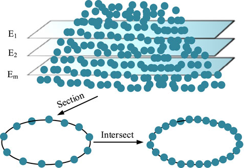
FIGURE 3. Schematic diagram of slicing in layered cutting.

As depicted in Figure 3, the complete point cloud data set is divided into multiple sections through multi-layer slicing operations. By intersecting the point cloud data of each section, an overview of the entire point cloud model can be obtained, and the computational expression of this process is shown in Formula (Huang et al., 2020).

$\left\{\begin{array}{l}{E}_1=E\max \\ E_2+\Delta dist=E\max \\ E_3+2\Delta dist=E\max \\ E_i+\left(i+1\right)\Delta dist=E\max \\ E_m+\left(m-1\right)\Delta dist=Emax\end{array}\right.(3)$

In Formula 3 (Huang et al., 2020), $\Delta dist$ represents the distance between adjacent layers of slices, and $E_1,E_2,E_3,\cdots E_i,E_m$ represents the number of layers of slices. As scattered point clouds are discretely distributed, to further optimize the contour of the point cloud model, the study introduces the concept of slicing thickness. The relationship between the slicing plane and the slicing thickness is expressed in Formula (Praveen et al., 2020).

$\delta =\stackrel{`}{k}\rho (4)$

In Formula 4 (Praveen et al., 2020), $\delta$ represents the slicing thickness, $\rho$ represents point cloud density, and $\stackrel{`}{k}$ represents the adjustment coefficient. The slice thickness is a critical parameter whose numerical determination is inextricably linked to computational efficiency, point cloud density and machine performance. First, small slice thickness increases the number of tool trajectories, which may lead to a decrease in computational efficiency. Therefore, a trade-off between computational efficiency and machining accuracy is required. Secondly, a high density point cloud can use a relatively large slice thickness, while a low density point cloud may require a smaller slice thickness. Finally, choosing the right machine tool for machining can improve the efficiency and accuracy of slicing thicknesses. At this point, selecting a point $p$ within a section, the distance calculation formula between $p$ and a nearby point $m$ is expressed in Formula (Li et al., 2021).

$d=\sqrt{{\left(x-x_i\right)}^2+{\left(y-y_i\right)}^2+{\left(z-z_i\right)}^2}(5)$

In Formula 5 (Li et al., 2021), $x_i,y_i,z_i$ represents the 3D coordinates of point $p$, and $x,y,z$ represents the coordinates of point $m$. The calculation of point cloud density at this point is expressed in Formula (He et al., 2022).

$\rho ={\displaystyle \sum _i^N}{d}_{m,p}/N(6)$

In Formula 6 (He et al., 2022), $N$ represents randomly selected $N$ points, and $d_{m,p}$ represents the distance value between point $m$ and point $p$. Additionally, considering that point clouds lack a topological structure, it is necessary to first perform a two-dimensional grid division of the data for each section, followed by equidistant processing of the point cloud network. The two-dimensional (2D) meshing is further divided into mesh generation, coordinate transformation and data interpolation. Firstly, the point cloud data is projected onto a plane by a specific mesh generation algorithm to form a 2D mesh. Secondly, the 3D coordinates of the point cloud data are mapped to the 2D mesh coordinate system by means of coordinate transformation. Finally, for the uncovered areas of the grid, interpolation can be used to fill them, ensuring that there are corresponding data points on the entire 2D grid. After obtaining the extreme values of the section data, a 2D bounding grid perpendicular to the Z-axis is constructed using the coordinate extreme values. The number of grids on the X and Y-axes is expressed in Formula (Liu et al., 2020).

$\left\{\begin{array}{l}x\_num=floor\left(\left(x_{\max }-x_{\min }\right)/k\cdot \rho \right)+1\\ y\_num=floor\left(\left(y_{\max }-y_{\min }\right)/k\cdot \rho \right)+1\end{array}\right.(7)$

In Formula 7 (Liu et al., 2020), $floor(\left(x_{\max }-x_{\min }\right)$ represents the number of layers on the X-axis, and $floor(\left(y_{\max }-y_{\min }\right)$ represents the number of layers on the Y-axis. The grid position number of any point $p$ is denoted as $\left(a,b\right)$, and the expression is given in Formula (Liang et al., 2020).

$\left\{\begin{array}{l}a=\left(x_i-x_{\min }\right)/l\\ b=\left(y_i-y_{\min }\right)/l\end{array}\right.(8)$

In Formula 8 (Liang et al., 2020), $l$ represents the side length of a square grid. The grid with the extreme values calculated is referred to as the boundary grid. After equidistant processing and sorting of the boundary grid, the tool position grid is obtained. The sorting is based on the center point of each cell, and assuming the grid coordinates for the $a$-th row and $b$-th column are $S\left(x_s,y_s\right)$, the coordinate calculation formula is expressed in Formula (Gawali et al., 2021).

$\left\{\begin{array}{l}{x}_s=x_{\min }+a\times l-\frac{l}{2}\\ y_s=y_{\min }+b\times l-\frac{l}{2}\end{array}\right.(9)$

The algebraic meaning in Formula 9 (Gawali et al., 2021) is consistent with the previous explanation. Once the sorting process is completed, an equidistant processing can be performed. If $S\left(x_s,y_s\right)$ belongs to one of the maximum grids in column $b$, the sequentially corresponding grid index after equidistant processing is marked as $\left(a-1,b\right)$, forming the set $Q_r$. If $S\left(x_s,y_s\right)$ belongs to one of the minimum grids in column $b$, the corresponding grid index is marked as $\left(a+1,b\right)$ and denoted as $Q_r$. The initial cutting grid then becomes the union of $Q_r$ and $Q_r$. In summary, after evaluating and updating all cutting positions and combining them with row cutting, it forms the entire movement path of the rough machining tool positions. The schematic diagram of the tool path for rough machining at this point is depicted in Figure 4.

FIGURE 4

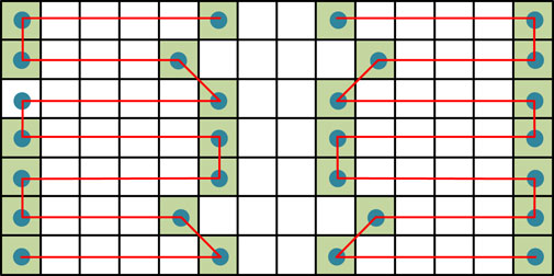
FIGURE 4. Schematic diagram of rough machining tool path.

As depicted in Figure 4, a specific layer is treated as an example involves intersecting the cutting grid. This is achieved by drawing lines parallel to the X-axis and passing through the center of each grid. The outcome of this process is the generation of segmented cutting tool lines after truncation. The tool trajectory connects these lines in a zigzag pattern from left to right and bottom to top, starting from the bottom-left grid. Connecting the right-side tool trajectory using the same method and joining them together provides the complete trajectory for the rough machining tool. In summary, the integration of layer cutting method into the trajectory planning of roughing point cloud model in practical application is roughly divided into four steps. The first step is data preparation, i.e., selecting appropriate workpieces, ensuring that their point cloud data can contain complex geometric information, and collecting the point cloud data by high-quality 3D scanning equipment (e.g., laser scanner), setting appropriate resolution and sampling density. The next is data preprocessing, where the acquired information is denoised by four-point noise reduction to smooth the data. Then the layer cutting method is implemented to describe the layer cutting path generation of the point cloud data, set the thickness parameter, etc. Finally, the simulation test is conducted with specific engineering examples to verify the effect of the layer cutting roughing method.

3.3 Generation of finish machining tool paths based on point cloud models

Continuing the exploration into generating CNC milling machine finish machining tool paths, the research focuses on the field of five-axis machining using point cloud models. The specific path generation involves employing the equal residual height method. A typical schematic diagram of the equal residual height method is illustrated in Figure 5.

FIGURE 5

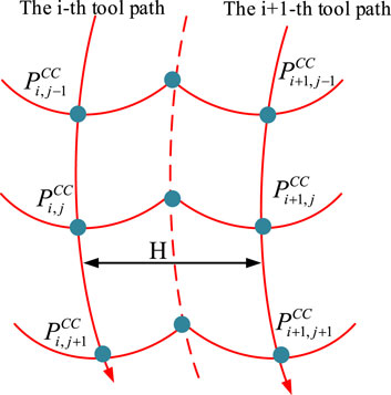
FIGURE 5. Schematic diagram of traditional equal residual height method.

From Figure 5, it’s evident that initially, the longest scanning line within the point cloud boundary is selected as the first tool path. Subsequently, under the constraint of the residual height preset value, the tool contact points for adjacent rows are calculated and connected to form a complete tool path. In this case, the residual height represents the distance from the point to the surface of the workpiece and can be obtained by simple geometric calculations. The residual height threshold, on the other hand, is an important parameter that determines which residual heights are considered valid surfaces for machining. While this method can simulate tool path generation, the repetitive steps involved in practical operations increase the computational load of the algorithm. Hence, the study attempts to perform spatial grid processing on point cloud data, creating bounding boxes. The formula for calculating the point cloud model’s bounding box in polar coordinates within the spatial grid is shown in Formula (Liu et al., 2022).

$\left\{\begin{array}{l}x`\_num=floor\left(\left(x_{\max }-x_{\min }\right)/k\cdot \rho \right)+1\\ y`\_num=floor\left(\left(y_{\max }-y_{\min }\right)/k\cdot \rho \right)+1\\ z`\_num=floor\left(\left(z_{\max }-z_{\min }\right)/k\cdot \rho \right)+1\end{array}\right.(10)$

In Formula 10 (Liu et al., 2022), $\stackrel{`}{x}\_num$, $\stackrel{`}{y}\_num$, and $\stackrel{`}{z}\_num$ represent the number of grids along the X-axis, Y-axis, and Z-axis in the spatial grid, respectively. At this point, in the bounding box, a column is arbitrarily selected, and the data in that column are denoted as $p_i^L$. After selecting all the boundaries of this column and calculating the arch height error, the tool contact points for the first tool path can be derived. The computational formula for this process is shown in Formula (Sheng et al., 2022).

$x_{\min }+\left(i-1\right)\cdot k\cdot \rho \le p\cdot x\le x_{\min }+i\cdot k\cdot \rho (11)$

In Formula 11 (Sheng et al., 2022), the range of values for $i$ is $1\le i\le \stackrel{`}{x}\_num$. The point with the minimum Y-coordinate in $p_i^L$ is selected as the boundary point $p_i^{BD}$. Only when $i=\stackrel{`}{x}\_num$, all the boundary points can form a complete set. The calculation formula for this process is given in Formula (Sales et al., 2021).

$\epsilon `=\frac{\left|\left(p_j^{BD}\cdot z-p_{j+n}^{BD}\cdot z\right)x_k+\left(p_j^{BD}\cdot x-p_{j+n}^{BD}\cdot x\right)z_k-\left(p_j^{BD}\cdot x\right)\cdot \left(p_{j+n}^{BD}\cdot z\right)\right|}{\sqrt{{\left(p_{j+n}^{BD}\cdot z-p_j^{BD}\cdot z\right)}^2+{\left(p_j^{BD}\cdot x-p_{j+n}^{BD}\cdot x\right)}^2}}(12)$

In Formula 12 (Sales et al., 2021), $p_j^{BD}$ represents the $j$ th point in the boundary set, and $p_{j+n}^{BD}$ represents the $j+n$ th point in the boundary set. $\stackrel{`}{\epsilon }$ represents the general length of the line connecting $p_j^{BD}$ and $p_{j+n}^{BD}$, and the midpoint of this line is $p_k^{BD}$. The definition of tool contact point judgment at this point is given by Formula (Nirala and Agrawal, 2020).

$\left\{\begin{array}{l}{p}_1=p_{j+n-1}^{BD},\epsilon `>e\\ p_2=p_{j+n+1}^{BD},\epsilon `<e\\ ⋮\\ p_1=p_{i,j}^{CC}\cup p_2=p_{i,j+1}^{CC},\epsilon `=e\end{array}\right.(13)$

In Formula 13 (Nirala and Agrawal, 2020), $e$ represents the bow height error, $p_{i,j}^{CC}$ and $p_{i,j+1}^{CC}$ respectively represent the tool contact points of the $j$ th and $j+1$ th points in the $i$ th column. The calculation of subsequent tool contact points continues based on the inference in the Formula, and finally, they are connected to form the first tool contact trajectory. This tool contact trajectory can be used to obtain the tool position trajectory for the first tool path. The tool contact point continues to update to $p_{i,j+1}^{CC}$ until all tool contact points have undergone coordinate calculations. The tool position points and tool axis vectors during tool processing can be obtained from these coordinates. To summarize, the study preprocesses the point cloud data. Filtering, denoising and other operations are carried out before transforming the coordinate value mapping. Then the point cloud model is processed by the residual height method, the residual height value is calculated, and the finishing toolpath planning is obtained after filtering and threshold setting, as shown in Figure 6.

FIGURE 6

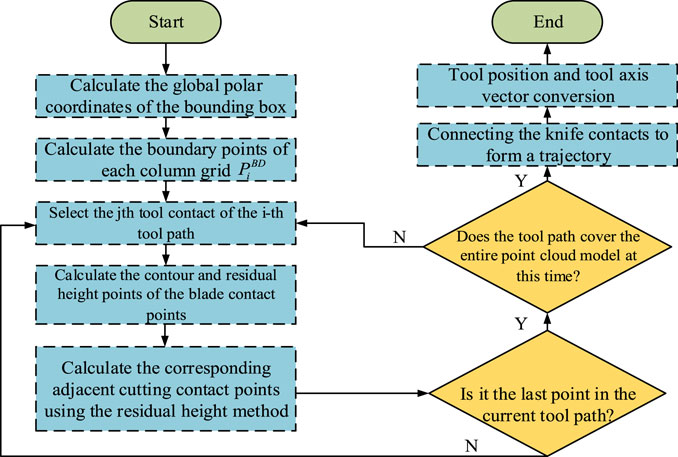
FIGURE 6. Process for generating tool paths for finish machining with equal residual height.

From Figure 6, it can be observed that the first step is to calculate the global coordinate extremes of the bounding box and select the Jth tool contact point of the Ith tool path. A local coordinate system is established based on this, and the contour point set and residual height value of this tool contact point are calculated. The adjacent row tool contact points are calculated using the residual height method. This process is repeated until all tool contact point calculations are completed. If, at this point, the tool path has covered the entire point cloud model, each path is connected to form the tool contact trajectory. Finally, the conversion of tool position points and tool axis vectors yields specific trajectory data. If the tool path has not yet covered the point cloud model, the next path is selected, and the process is continued. In summary, the integration of the residual height method into the trajectory planning of the finishing point cloud model in practice is also roughly divided into four steps. The first step is data preparation, i.e., selecting appropriate workpieces, ensuring that the point cloud data contains surfaces that need to be finely machined, and using high-precision 3D scanning equipment to obtain detailed surface information. Next is data preprocessing, where the collected point cloud data is denoised to ensure that the calculation of the residual height is not interfered by noise. Then comes the implementation of the residual height method, which calculates the residual height values and computes the path generation. Finally, an engineering example is cited for performance simulation test to evaluate the actual effect of residual height method finishing.

4 CNC milling tool path generation technique based on point cloud model testing

To validate the practicality and effectiveness of both the rough machining tool path generation method and the finish machining tool path generation method, performance and simulation tests were conducted on these two methods. Performance differences between the proposed methods and similar methods were further examined using indicators such as computation time, trajectory error, and residual height values.

4.1 Performance testing of rough machining technique

To verify the effectiveness of the proposed method for generating rough machining tool paths using a point cloud model, simulations were conducted on a portion of the saddle surface using MATLAB. The point cloud data dimensions were set to 108 mm × 45 mm × 25 mm, and rough machining was performed using a flat-bottom cutter D6 with a radius of 5 mm. The distance between adjacent layers of slices was set to 0.5 mm. Different slice thicknesses ${\delta }_1=3mm$, ${\delta }_2=4mm$, ${\delta }_3=5mm$, and ${\delta }_4=6mm$ were considered as variables. The actual trajectory generated by the proposed method is shown in Figure 7.

FIGURE 7

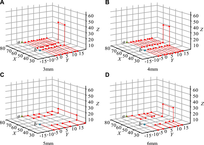
FIGURE 7. Comparison of 3D trajectories of roughing tools with different slice thicknesses.

Figure 7 illustrated the toolpaths under different thicknesses. Figure 7A represents the toolpath for a thickness of 3 mm, Figure 7B for 4 mm, Figure 7C for 5 mm, and Figure 7D for 6 mm. As observed from Figure 7, comparing the toolpaths for four different slicing thicknesses revealed that smaller slicing thickness led to an increase in the number of cross-sectional planes during point cloud data slicing, subsequently resulting in longer algorithm computation times. Moreover, if the slicing thickness was too large, it increased the number of tool contact points within each slice after conversion. Therefore, after comprehensive evaluation based on tool contact points and path length, the slicing thickness of 5 mm in Figure 7 yields the optimal trajectory generation, and subsequent tests were conducted using this thickness. To validate the proposed point cloud model layer slicing method against existing machining methods, such as equidistant cutting and unit cutting, the study conducted comparative tests using trajectory error rate and computation time as reference indicators, as depicted in Figure 8.

FIGURE 8

FIGURE 8. Comparison of error rate and computing time tests for different roughing trajectory generation methods.

Figure 8A displays the error change rate curves for three different trajectory generation methods, while Figure 8B shows the computation time curves. It was evident from Figure 8 that the trajectory generation error for all three methods decreased with an increase in the number of tool contact points. Throughout this process, the proposed layer slicing method performed optimally, with the lowest error approaching 10%. Additionally, the layer slicing method exhibited the least computation time, with an average of approximately 35 s. These data indicate that 2D gridization of point cloud data using the layer slicing method can reduce the complexity of computation. In order to compare the performance effect of the three methods more accurately, the study tries to show the detail maps generated by the trajectories of these methods in X-O-Y planar projection as shown in Figure 9.

FIGURE 9

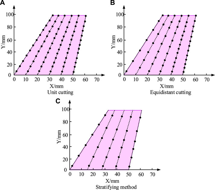
FIGURE 9. Comparison of X-O-Y plane projection details of three methods.

Figure 9A shows the trajectory projection of the unit cutting method, Figure 9B shows the trajectory projection of the isometric cutting method, and Figure 9C shows the trajectory projection of the layer cutting method. As can be seen from Figure 9, the number of trajectory paths of both unit cutting method and isometric cutting method was 6, and the number of tool contacts was obviously more than layer cutting method. The roughing of the workpiece by the layer cutting method produced only 5 trajectory paths, and the number of tool contacts was even less. The reason for this difference may be attributed to unit cutting dividing the workpiece into multiple units for sequential cutting, thereby generating more trajectory lines. Isometric cutting, on the other hand, mechanically made planning more difficult by calculating the distance between tool contacts. Furthermore, the layer slicing method had significantly fewer tool contact points than the unit cutting method, maintaining the overall machining structure unchanged. This can greatly reduce the data computation time for the point cloud model, ultimately optimizing the cutting process.

4.2 Performance testing of finish machining technology

To validate the effectiveness of the proposed finish machining toolpath generation method, tests were conducted using MATLAB 2019a as the simulation software. The simulation involved 168,900 scattered points, and the effective cutting radius of the circular milling cutter was set to 4 mm. Residual height was set to 0.6 mm, bow height error to 0.05 mm, forward tilt angle to 10°, and lateral offset angle to 0°. Using a surface point cloud model as an example, the proposed method was tested against existing finish machining cutting methods such as polyhedron, projection, and offset surface methods, and the results are presented in Figure 10.

FIGURE 10

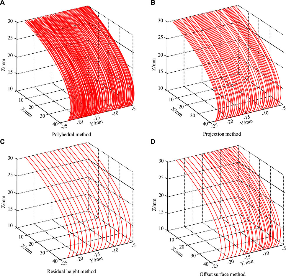
FIGURE 10. Comparative analysis of 3D trajectories of different finishing tools.

Figure 10A depicts the toolpath of the point cloud model under the polyhedron method, Figure 10B under the projection method, Figure 10C under the residual height method, and Figure 10D under the offset surface method. From Figure 10, it was observed that, in the segmentation of path data for the surface point cloud model, the polyhedron method exhibited complexity and multiple paths. Although the projection method showed improvement in trajectory generation, there were still instances of path crossings. The offset surface method enhanced the trajectory planning, but unevenness and bias persisted. Overall, the proposed residual height method performed optimally, demonstrating a certain superiority in model path generation. To further explore the machining effects of the residual height method, sampling along the residual height line was conducted, and the obtained residual heights are shown in Figure 11.

FIGURE 11

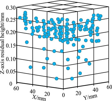
FIGURE 11. Analysis of residual height on the surface of workpieces.

From Figure 11, it was evident that, after obtaining the sampling space coordinates with unchanged X and Y-axes, the Z-axis coordinates transformed by the residual height method mainly concentrated in the intervals of 0.2–0.25 and 0.25–0.3, while the remaining residual heights were scattered below 0.2. This indicates that the residual height method achieved an efficiency of over 60% in toolpath generation for finish machining workpieces, simultaneously avoiding the complex processes of surface fitting and triangulation, streamlining the steps of path generation. Finally, the study, in order to verify the practical application effect of the new roughing and finishing trajectory generation method, compared and verified the traditional finishing and improved finishing, and the traditional roughing and improved roughing, respectively, with H7 helical gears, HK1712 needle roller bearings, and M6 double-ended zinc-plated screws as the test parts, and the physical drawings are shown in Figure 12.

FIGURE 12

FIGURE 12. Physical schematics of the three test parts.

Figure 12A shows the physical drawing of H7 helical gear, Figure 12B shows the physical drawing of HK1712 needle roller bearing, and Figure 12C shows the physical drawing of M6 double-ended galvanized screw. In addition, the study set the roughing tool diameter to φ12 and finishing to φ6. The lathe speed settings were set to 3,500 m/s and 4,500 m/s, and the feeds were set to 1,000 and 800 mm/r. The cutting pitch was set to 1.2 mm and 4 mm, respectively. Furthermore, more machining methods of the same type were introduced, such as the grid of the same type as the layer cut roughing method cutting, contour cutting, and lithographic cutting, and adaptive cutting, topology optimization, and dynamic cutting, which are the same type as the residual height method for finishing. Trajectory generation error rate, computing time, trajectory smoothness and cutting efficiency were tested as reference indexes, and the test results are shown in Table 1.

TABLE 1

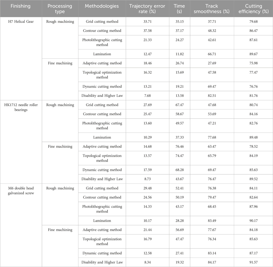
TABLE 1. Test results of different finishing methods.

As can be seen from Table 1, all 16 processing methods showed superior processing results in the multi-indicator test. Firstly, for the rough machining method comparison, the layer cutting method proposed in the study showed the best overall performance. This was followed by the photolithography cutting method, the contour cutting method and the grid cutting method. Comprehensively, the layer cutting roughing method had the lowest trajectory generation error rate of 10.17% in M6 double-ended galvanized screw, the lowest running time of 11.82s in H7 helical gear machining, the highest value of trajectory smoothness of 83.49% in M6 double-ended galvanized screw machining, and the highest cutting efficiency of 90.17% in M6 double-ended galvanized screw machining. On the contrary, the residual high finish machining method showed the lowest trajectory generation error rate of 7.68% in H7 helical gear machining, the lowest running time of 13.58 s in H7 helical gear machining, the highest value of trajectory smoothing of 84.17% in M6 double-head galvanized screw machining, and the highest cutting efficiency of 91.57% in M6 double-head galvanized screw machining. In summary, the proposed method of generating finishing tool trajectories using the residual height method to compute the point cloud model showed better performance and certain feasibility compared to the same type of arithmetic methods.

5 Conclusion

In recent years, numerous researchers have proposed various technical models to simulate the generation of CNC toolpaths. To further explore the application effectiveness of data models in this field, the study introduced a point cloud model and performed preprocessing, denoising, and down-sampling on the point cloud data. Toolpath generation methods for rough machining and finish machining were proposed using the point cloud model. Experimental results indicated that the method of generating rough machining toolpaths using the layering method for calculating the point cloud model was the shortest under specific slicing thickness. The trajectory generated by the layering method had an error close to 10%, with an average computation time of approximately 35 s. Compared to similar rough machining methods, this approach produced shorter trajectories with lower algorithmic complexity. In performance testing of the finish machining toolpath generation method using the residual height method to calculate the point cloud model, the toolpaths generated by the residual height method were more uniform, shorter, and exhibited higher parallelism. Analysis of residual heights sampled from the workpiece surface revealed concentrations in the range of 0.2–0.3, with a generation efficiency of at least 60%. In comparison to other similar finish machining methods, this method achieved a minimum trajectory error rate of 10.17%, a minimum computation time of 11.82 s, a maximum trajectory smoothness of 83.49%, and a maximum cutting efficiency of 90.17%. In summary, the two proposed trajectory generation methods in the study enable efficient, precise, and sustainable CNC milling machine operations. However, the trajectory generation methods demonstrated in the research have a high requirement for point cloud density. When the point cloud density is sparse, there is uncertainty in the computation results. Therefore, future research could continue to explore trajectory generation methods for light-density point clouds to enhance the computational integrity of point cloud models.

Data availability statement

The original contributions presented in the study are included in the article/Supplementary Material, further inquiries can be directed to the corresponding author.

Author contributions

JL: Conceptualization, Data curation, Project administration, Writing–original draft. ZH: Formal Analysis, Methodology, Writing–review and editing.

Funding

The author(s) declare that no financial support was received for the research, authorship, and/or publication of this article.

Conflict of interest

The authors declare that the research was conducted in the absence of any commercial or financial relationships that could be construed as a potential conflict of interest.

Publisher’s note

All claims expressed in this article are solely those of the authors and do not necessarily represent those of their affiliated organizations, or those of the publisher, the editors and the reviewers. Any product that may be evaluated in this article, or claim that may be made by its manufacturer, is not guaranteed or endorsed by the publisher.

References

Chen, Y., Zhang, Y., and Zhang, F. (2021). Personalized path generation and robust H∞ output-feedback path following control for automated vehicles considering driving styles. IET Intell. Transp. Syst. 15 (12), 1582–1595. doi:10.1049/itr2.12097

CrossRef Full Text | Google Scholar

Choudhuri, S., Adeniye, S., and Sen, A. (2023). Distribution alignment using complement entropy objective and adaptive consensus-based label refinement for partial domain adaptation. Artif. Intell. Appl. 1 (1), 43–51. doi:10.47852/bonviewaia2202524

CrossRef Full Text | Google Scholar

Gawali, D. D., Patil, B. V., Zidna, A., and Nataraj, P. V. S. (2021). Constrained global optimization of multivariate polynomials using polynomial B-spline form and B-spline consistency prune approach. RAIRO - Operations Res. 55 (6), 3743–3771. doi:10.1051/ro/2021179

CrossRef Full Text | Google Scholar

He, W., Shi, J., Su, T., Lu, Z., Hao, L., and Huang, Y. (2021). Automated test generation for IEC 61131-3 ST programs via dynamic symbolic execution. Sci. Comput. Program. 206 (1), 102608–102609. doi:10.1016/j.scico.2021.102608

CrossRef Full Text | Google Scholar

He, Z., Fang, H., Bao, Y., Yang, F., and Zhang, J. (2022). Smooth toolpath interpolation for a 5-axis hybrid machine tool. Robotica 40 (12), 4431–4454. doi:10.1017/s026357472200100x

CrossRef Full Text | Google Scholar

Huang, N., Jin, Y., and Lu, Y. (2020). Spiral toolpath generation method for pocket machining. Comput. Industrial Eng. 60 (12), 340–355. doi:10.1016/j.cie.2019.106142

CrossRef Full Text | Google Scholar

Leal, E., Sanchez-Torres, G., and Branch, J. W. (2020). Sparse regularization-based approach for point cloud denoising and sharp features enhancement. Sensors 20 (11), 3206–3207. doi:10.3390/s20113206

PubMed Abstract | CrossRef Full Text | Google Scholar

Li, Z., and Tang, K. (2021). Partition-based five-axis tool path generation for freeform surface machining using a non-spherical tool. J. Manuf. Syst. 58 (7), 248–262. doi:10.1016/j.jmsy.2020.12.004

CrossRef Full Text | Google Scholar

Li, Z., Yan, Q., and Tang, K. (2021). Multi-pass adaptive tool path generation for flank milling of thin-walled workpieces based on the deflection constraints. J. Manuf. Process. 68 (8), 690–705. doi:10.1016/j.jmapro.2021.05.075

CrossRef Full Text | Google Scholar

Liang, F., Kang, C., and Fang, F. (2020). A smooth tool path planning method on NURBS surface based on the shortest boundary geodesic map. J. Manuf. Process. 58 (1), 646–658. doi:10.1016/j.jmapro.2020.08.047

CrossRef Full Text | Google Scholar

Liu, C., Li, Y., Jiang, X., and Shao, W. (2020). Five-axis flank milling tool path generation with curvature continuity and smooth cutting force for pockets. Chin. J. Aeronautics 33 (2), 730–739. doi:10.1016/j.cja.2018.12.003

CrossRef Full Text | Google Scholar

Liu, X., Liu, Z., Huang, H. Z., Zhu, P., and Liang, Z. (2022). A new inherent reliability modeling and analysis method based on imprecise Dirichlet model for machine tool spindle. Ann. Operations Res. 311 (1), 295–310. doi:10.1007/s10479-019-03333-9

CrossRef Full Text | Google Scholar

Nirala, H. K., and Agrawal, A. (2020). Reprint of: residual stress inclusion in the incrementally formed geometry using fractal geometry based incremental toolpath (FGBIT). J. Mater. Process. Technol. 287 (9), 116623–116624. doi:10.1016/j.jmatprotec.2020.116623

CrossRef Full Text | Google Scholar

Praveen, K., Lingam, R., and Reddy, N. V. (2020). Tool path design system to enhance accuracy during double sided incremental forming: an analytical model to predict compensations for small/large components. J. Manuf. Process. 58 (12), 510–523. doi:10.1016/j.jmapro.2020.08.014

CrossRef Full Text | Google Scholar

Sales, E., Kwok, T. H., and Chen, Y. (2021). Function-aware slicing using principal stress line for toolpath planning in additive manufacturing. J. Manuf. Process. 64 (4), 1420–1433. doi:10.1016/j.jmapro.2021.02.050

CrossRef Full Text | Google Scholar

Sheng, P., Xiao, Z., and Dong, L. (2022). Design of a control system of plane machining machine tool based on machine vision. China Foundry 29 (6), 784–792. doi:10.3785/j.issn.1006-754X.2022.00.078

CrossRef Full Text | Google Scholar

Zheng, Z., Zha, B., Zhou, Y., Huang, J., Xuchen, Y., and Zhang, H. (2022). Single-stage adaptive multi-scale point cloud noise filtering algorithm based on feature information. Remote Sens. 14 (2), 367–368. doi:10.3390/rs14020367

CrossRef Full Text | Google Scholar