Vehicle lateral tracking control optimization based on fuzzy preview time and ant lion algorithm

To enhance the path tracking performance of intelligent vehicles, this paper conducts optimization research on the classical Linear Quadratic Regulator (LQR) controller based on a 2-degrees-of-freedom (2-DOF) vehicle dynamics lateral tracking error model. Aiming at the insufficient adaptability of the LQR controller with fixed weight coefficients at varying vehicle speeds, the Ant Lion Optimizer (ALO) is introduced to dynamically adjust the matrix weight coefficients, and a preview feed-forward steering angle compensation strategy is integrated to improve the lateral path-tracking capability. Furthermore, to address the reduced steering stability of the feed-forward LQR controller caused by model linearization, an adaptive prediction mechanism based on fuzzy control is designed. This mechanism integrates parameters such as vehicle speed, path curvature, and its rate of change. By utilizing a dual-fuzzy controller, a hybrid control strategy that combines dynamic prediction time and fixed preview time is constructed. Simulation verification is conducted via MATLAB/Simulink and CarSim co-simulation. Results show the proposed lateral control method balances tracking accuracy and system stability, with good robustness across speeds—simulation at double lane change 95.66% lower than traditional LQR at 15 m/s , and only 39.74% of traditional LQR's average deviation at 25 m/s. This study offers an efficient solution for intelligent vehicle lateral tracking, addressing fixed-weight LQR and fixed preview time limitations in complex roads.

1 Introduction

Intelligent vehicles refer to a new generation of vehicles equipped with advanced sensors and other devices, utilizing new technologies such as artificial intelligence, featuring autonomous driving capabilities, and gradually developing into intelligent mobile spaces and application terminals (Zhang et al., 2020). With the rapid advancement of autonomous driving technology, intelligent vehicles have been gradually deployed in specific fields such as environmental sanitation services, transportation, and industrial parks (Cui et al., 2022), significantly transforming people’s lifestyles and quality of life. In the future, higher-level autonomous driving will offer broad application prospects. Generally, an autonomous driving system consists of four components: environmental perception, decision-making, path planning, and path tracking (Hu et al., 2021). Among these technologies, path tracking control is the core of realizing intelligent driving and effectively ensures vehicle driving safety and handling stability (Ribeiro et al., 2020). Since it directly affects vehicle safety and user experience, path tracking technology has great value in engineering applications and profound significance for theoretical research.

Currently, scholars have focused on path tracking research based on vehicle dynamics, and the main methods widely used in lateral tracking control include fuzzy control (Zhou et al., 2025), Linear Quadratic Regulator (LQR) (Kaleemullah and Faris, 2022), and Model Predictive Control (MPC) (Norouzi et al., 2023). Among these, LQR control is extensively used in lateral control of vehicle trajectory tracking due to not requiring online optimization calculations, thus saving a large amount of computing resources, and exhibiting high practical application value in real vehicles under embedded environments (Wang et al., 2020).

During path tracking, vehicle speed and planned path curvature are not fixed, and both have a significant impact on the control effect of the path tracking controller. Therefore, the LQR controller with fixed weights is difficult to ensure the optimal path tracking effect under different vehicle speeds and road curvatures, which greatly limits the adaptability and accuracy of the controller. Guo Ningyuan et al. also found in their research on the handling stability of distributed drive electric vehicles that the fixed feedback gain of the Linear Quadratic Regulator (LQR) cannot achieve adaptive adjustment like nonlinear model predictive control (NMPC). It is difficult to cope with physical constraints and stability requirements under dynamic operating conditions, and may even lead to vehicle instability (Zhang et al., 2024). Thus, research on variable weight matrices Q and R has gradually developed. Improvements to the LQR lateral tracking controller based on fuzzy controllers (Hu et al., 2022), genetic algorithms (Gong et al., 2023), particle swarm optimization (PSO) (Wang X. G. et al., 2024), and ant lion optimization algorithms (Wang et al., 2023) have achieved higher tracking accuracy to varying degrees. Compared with other swarm intelligence optimization algorithms (such as genetic algorithms and particle swarm optimization), the ALO algorithm has stronger optimization convergence ability. In addition, ALO is more convenient and intuitive to apply due to fewer parameters to adjust, so this study selects the ant lion algorithm to optimize the matrix weights.

According to different control strategies, trajectory tracking can be divided into two categories: preview strategy-based (Chen et al., 2014) and non-preview strategy-based (Guo et al., 2019). Research has shown that preview-based strategies achieve better performance in trajectory tracking. To enable trajectory tracking to adapt to different paths, taking the vehicle’s speed and curvature as inputs to realize optimization the preview distance (Li et al., 2024; Li and Chen, 2024; Ibrahim, 2022; Wang F. A. et al., 2024) can significantly improve tracking accuracy. Cui Kaichen et al. (Cui et al., 2024) designed an adaptive preview time controller based on vehicle speed and road curvature using a fuzzy control algorithm, in order to select the optimal prediction time T to adapt to various road conditions. Shi Qiang et al. (Shi et al., 2021) incorporate the curvature change rate as a factor affecting trajectory tracking accuracy, used the unit length curvature increment after mean filtering to describe the curvature fluctuation, and dynamically adjusted the normalized parameters of pure tracking control and feed-forward control. Therefore, based on the fuzzy controller in (Cui et al., 2024), this study improves the fuzzy controller according to the curvature change rate of the reference trajectory.

In summary, to tackle the problem of poor control adaptability caused by fixed weight coefficients, this study dynamically adjusts the weight coefficients of the LQR lateral tracking controller based on the ALO algorithm. On the basis of the controller that optimizes the preview time using speed and curvature, a dual-fuzzy controller is designed according to the curvature change rate, and a hybrid control strategy combining real-time changing and fixed preview time is adopted to reduce the calculation time. Finally, MATLAB/Simulink and CarSim co-simulation are conducted to verify the trajectory tracking effect under two conditions. The results show that under different vehicle speeds, the hybrid controller significantly improves the optimization effect in terms of distance deviation, side slip angle of the center of mass, and yaw rate.

The subsequent chapters of this paper are organized as follows: Chapter 2 focuses on Materials and Methods, providing a detailed account of the construction of the 2-DOF vehicle dynamics model, the design of the LQR controller, and the optimization methods based on the ALO and fuzzy control. Chapter 3 is dedicated to Experimental Scenario Settings and Evaluation Indicators. It defines the simulation platform, comparative controllers, experimental scenarios, vehicle speed parameters, and performance evaluation indicators. Chapter 4 presents Simulation Results and Analysis. It compares the performance of different controllers under double lane change and double sine trajectory scenarios, so as to verify the effectiveness of the proposed method. Chapter 5 contains Conclusions and Prospects. It summarizes the research findings, analyzes the existing limitations, and puts forward directions for future research.

2 Materials and methods

2.1 Vehicle dynamics model

2.1.1 Assumptions and parameter definition

This paper adopts a simplified 2-DOF vehicle dynamic model with the following assumptions:

1. The vehicle is symmetric about its longitudinal axis, with its center of mass (COM) at the coordinate origin, and the effect of wheel track is neglected;

2. Only planar motion is considered, and ignoring vertical motion;

3. The tires are assumed to be rigid; the effects of the suspension, air resistance, and rolling resistance are neglected.

When the vehicle is traveling at high speeds, it is assumed that the tires undergo no deformation and the slip angle is zero, meaning the lateral force exhibits a linear relationship with the slip angle ($F_{\mathrm{y}}=C\alpha$). Based on the bicycle model (see Figure 1):

Figure 1

Figure 1. Two-degree-of-freedom vehicle dynamics model.

2.1.2 Establishment of dynamic equations

Based on Newton’s second law, under the assumption of small angles, the 2-DOF dynamic equations are established in Equation 1:

$\left\{\begin{array}{l}\mathit{m}{\mathit{a}}_{\mathit{y}}={\mathit{F}}_{\mathit{y}\mathit{f}}+{\mathit{F}}_{\mathit{y}\mathit{r}}={\mathit{C}}_{\mathit{\alpha }\mathit{f}}{\mathit{\alpha }}_{\mathit{f}}+{\mathit{C}}_{\mathit{\alpha }\mathit{r}}{\mathit{\alpha }}_{\mathit{r}}\\ {\mathit{I}}_{\mathit{z}}\ddot{\mathit{\psi }}={\mathit{F}}_{\mathit{y}\mathit{f}}{\mathit{l}}_{\mathit{f}}-{\mathit{F}}_{\mathit{y}\mathit{r}}{\mathit{l}}_{\mathit{r}}={\mathit{l}}_{\mathit{f}}{\mathit{C}}_{\mathit{\alpha }\mathit{f}}{\mathit{\alpha }}_{\mathit{f}}-{\mathit{l}}_{\mathit{r}}{\mathit{C}}_{\mathit{\alpha }\mathit{r}}{\mathit{\alpha }}_{\mathit{r}}\\ {\mathit{a}}_{\mathit{y}}=\ddot{\mathit{y}}+{\mathit{v}}_{\mathit{x}}\dot{\mathit{\psi }}\\ {\mathit{v}}_{\mathit{y}}=\dot{\mathit{y}}\end{array}\right.(1)$

Where $\mathrm{m}$ is the total mass of the vehicle, $\mathrm{\psi }$ is the yaw angle, and ${\mathrm{I}}_{\mathrm{z}}$ is the moment of inertia about the z-axis. From this, the motion equations of the 2-DOF model can be derived as Equation 2:

$\left[\begin{array}{c}{\dot{\mathit{v}}}_{\mathit{y}}\\ \dot{\mathit{\omega }}\end{array}\right]=\left[\begin{array}{c}\ddot{\mathit{y}}\\ \ddot{\mathit{\psi }}\end{array}\right]=\left[\begin{array}{cc}\frac{C_{\alpha f}+C_{\alpha r}}{m{v}_x}& \frac{l_f{C}_{\alpha f}-l_r{C}_{\alpha r}}{m{v}_x}-v_x\\ \frac{l_f{C}_{\alpha f}-l_r{C}_{\alpha r}}{I_z{v}_x}& \frac{l_f^2{C}_{\alpha f}+l_r^2{C}_{\alpha r}}{I_z{v}_x}\end{array}\right]\left[\begin{array}{c}{\dot{\mathit{v}}}_{\mathit{y}}\\ \dot{\mathit{\psi }}\end{array}\right]+\left[\begin{array}{c}-\frac{C_{\alpha f}}{m}\\ -\frac{l_f{C}_{\alpha f}}{I_z}\end{array}\right]\delta (2)$

In the above equations, ${\mathrm{C}}_{\alpha \mathrm{f}}$ and ${\mathrm{C}}_{\alpha \mathrm{r}}$ represent the side slip stiffness of the front and rear wheels, respectively, and ${\mathrm{v}}_{\mathrm{x}}=\text{vcos}\left(\mathrm{\beta }\right)$ and ${\mathrm{v}}_{\mathrm{y}}=\text{vsin}\left(\mathrm{\beta }\right)$ are the components of the vehicle’s velocity at the center of mass along the x, y directions in the vehicle coordinate system. The Cartesian coordinate system makes it difficult to intuitively describe path tracking error, so a transformation to the Frenet coordinate system is applied:

The lateral error is the distance between the current vehicle position and the projection point on the target path, while the heading angle error is the angle between the vehicle’s heading angle and the tangential direction of the path (see in Figure 2). In the figure, point $\mathrm{A}$ represents the actual position of the vehicle, and point ${\mathrm{A}}^{\prime }$ is the projection point of the vehicle on the target path $\overrightarrow{\mathit{S}}$ is the position vector of the vehicle’s actual location, and $\overrightarrow{{\mathit{S}}_{\mathit{r}}}$ is the vector of the projection point; $\dot{\mathit{s}}$ is the speed magnitude at the projection point of the vehicle on the target path; $\mathit{\theta }$ is the vehicle heading angle; and ${\mathit{\theta }}_{\mathit{r}}$ is the heading angle of the projection point on the target path. Based on the geometric relationships and Frenet formulas, the path tracking error model can be expressed as Equation 3:

${\dot{\mathit{e}}}_{\mathit{r}\mathit{r}}=\mathit{A}{\mathit{e}}_{\mathit{r}\mathit{r}}+\mathit{B}\mathit{u}+\mathit{C}{\dot{\mathit{\theta }}}_{\mathit{r}}(3)$

Figure 2

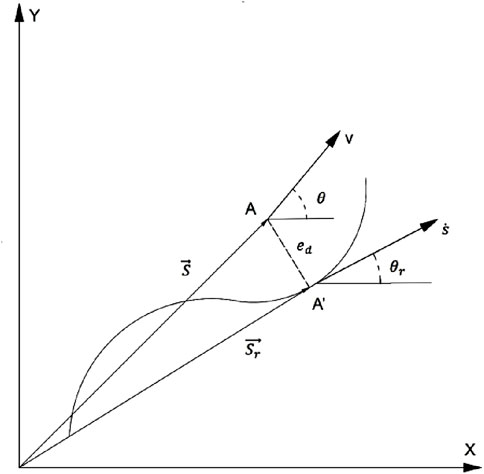
Figure 2. Path tracking error diagram.

In the equation, ${\dot{\mathit{e}}}_{\mathit{r}\mathit{r}}=\left[\begin{array}{cccc}{\mathit{e}}_{\mathit{d}}& {\dot{\mathit{e}}}_{\mathit{d}}& {\mathit{e}}_{\mathit{\phi }}& {\dot{\mathit{e}}}_{\mathit{\phi }}\end{array}\right]$ is the error vector, which includes the lateral error ${\mathit{e}}_{\mathit{d}}$ and its derivative ${\dot{\mathit{e}}}_{\mathit{d}}$, while ${\mathit{e}}_{\mathit{\phi }}$ and ${\dot{\mathit{e}}}_{\mathit{\phi }}$ represent the heading angle error and its derivative, respectively; $\mathrm{u}=\mathrm{\delta }$ is the control input; and $\mathbf{A}$, $\mathbf{B}$, and $\mathbf{C}$ are coefficient matrices.

$\mathit{A}=\left[\begin{array}{cccc}\mathbf{0}& \mathbf{1}& \mathbf{0}& \mathbf{0}\\ \mathbf{0}& -\frac{\mathbf{2}{\mathit{C}}_{\mathit{\alpha }\mathit{f}}+\mathbf{2}{\mathit{C}}_{\mathit{\alpha }\mathit{r}}}{\mathit{m}{\mathit{v}}_{\mathit{x}}}& \frac{\mathbf{2}{\mathit{C}}_{\mathit{\alpha }\mathit{f}}+\mathbf{2}{\mathit{C}}_{\mathit{\alpha }\mathit{r}}}{\mathit{m}}& -\frac{\mathbf{2}{\mathit{C}}_{\mathit{\alpha }\mathit{f}}{\mathit{l}}_{\mathit{f}}-\mathbf{2}{\mathit{C}}_{\mathit{\alpha }\mathit{r}}{\mathit{l}}_{\mathit{r}}}{\mathit{m}{\mathit{v}}_{\mathit{x}}}\\ \mathbf{0}& \mathbf{0}& \mathbf{0}& \mathbf{1}\\ \mathbf{0}& \frac{-\mathbf{2}{\mathit{C}}_{\mathit{\alpha }\mathit{f}}{\mathit{l}}_{\mathit{f}}-\mathbf{2}{\mathit{C}}_{\mathit{\alpha }\mathit{r}}{\mathit{l}}_{\mathit{r}}}{{\mathit{I}}_{\mathit{z}}{\mathit{v}}_{\mathit{x}}}& \frac{\mathbf{2}{\mathit{C}}_{\mathit{\alpha }\mathit{f}}{\mathit{l}}_{\mathit{f}}-\mathbf{2}{\mathit{C}}_{\mathit{\alpha }\mathit{r}}{\mathit{l}}_{\mathit{r}}}{{\mathit{I}}_{\mathit{z}}}& \frac{\mathbf{2}{\mathit{C}}_{\mathit{\alpha }\mathit{f}}{\mathit{l}}_{\mathit{f}}^{\mathbf{2}}-\mathbf{2}{\mathit{C}}_{\mathit{\alpha }\mathit{r}}{\mathit{l}}_{\mathit{r}}^{\mathbf{2}}}{{\mathit{I}}_{\mathit{z}}{\mathit{v}}_{\mathit{x}}}\end{array}\right],$

$\mathit{B}=\left[\begin{array}{c}\mathbf{0}\\ \frac{\mathbf{2}{\mathit{C}}_{\mathit{\alpha }\mathit{f}}}{\mathit{m}}\\ \mathbf{0}\\ \frac{\mathbf{2}{\mathit{C}}_{\mathit{\alpha }\mathit{f}}{\mathit{l}}_{\mathit{f}}}{{\mathit{I}}_{\mathit{z}}}\end{array}\right],\mathit{C}=\left[\begin{array}{c}\mathbf{0}\\ -{\mathit{v}}_{\mathit{x}}-\frac{\mathbf{2}{\mathit{C}}_{\mathit{\alpha }\mathit{f}}{\mathit{l}}_{\mathit{f}}-\mathbf{2}{\mathit{C}}_{\mathit{\alpha }\mathit{r}}{\mathit{l}}_{\mathit{r}}}{\mathit{m}{\mathit{v}}_{\mathit{x}}}\\ \mathbf{0}\\ \frac{\mathbf{2}{\mathit{C}}_{\mathit{\alpha }\mathit{f}}{\mathit{l}}_{\mathit{f}}^{\mathbf{2}}+\mathbf{2}{\mathit{C}}_{\mathit{\alpha }\mathit{r}}{\mathit{l}}_{\mathit{r}}^{\mathbf{2}}}{{\mathit{I}}_{\mathit{z}}{\mathit{v}}_{\mathit{x}}}\end{array}\right]$

2.2 LQR controller design

2.2.1 Feedback control law

LQR is an optimization control method based on state-space equations, widely used in lateral control of autonomous driving. Its core is to design an optimal control law to achieve the best balance between system state error and control input. The control objective is described by a quadratic cost function as Equation 4:

$\mathit{J}=\frac{\mathbf{1}}{\mathbf{2}}{\int }_{\mathbf{0}}^{\mathit{\infty }}\left[{\mathit{X}}^{\mathit{T}}\left(\mathit{t}\right)\mathit{Q}\mathit{X}\left(\mathit{t}\right)+{\mathit{U}}^{\mathit{T}}\left(\mathit{t}\right)\mathit{R}\mathit{U}\left(\mathit{t}\right)\right]\mathit{d}\mathit{t}(4)$

Where $\mathit{Q}$ and $\mathit{R}$ are controller weighting matrices, with $\mathit{Q}$ being positive definite or positive semi-definite and $\mathit{R}$ being positive definite. The Hamiltonian function as Equation 5 is constructed to solve for optimal control:

$\mathit{H}=\frac{\mathbf{1}}{\mathbf{2}}\left[{\mathit{X}}^{\mathit{T}}\mathit{Q}\mathit{X}+{\mathit{U}}^{\mathit{T}}\mathit{R}\mathit{U}\right]+{\mathit{\lambda }}^{\mathit{T}}\left(\mathit{A}\mathit{X}+\mathit{B}\mathit{U}\right)(5)$

By applying the extreme condition $\frac{\mathrm{\partial }\mathbf{H}}{\mathrm{\partial }\mathbf{U}}=0$, the optimal control input is derived as Equation 6:

${\mathit{U}}^{*}\left(\mathit{t}\right)=-{\mathit{R}}^{-\mathbf{1}}{\mathit{B}}^{\mathit{T}}\mathit{\lambda }\left(\mathit{t}\right)(6)$

Where $\mathit{\lambda }\left(\mathit{t}\right)=-\mathit{P}\left(\mathit{t}\right)\mathit{X}\left(\mathit{t}\right)$, $\mathbf{P}$ is the solution of the Riccati equation which is expressed as Equation 7:

$\mathit{P}\mathit{A}+{\mathit{A}}^{\mathit{T}}\mathit{P}-\mathit{P}\mathit{B}{\mathit{R}}^{-\mathbf{1}}{\mathit{B}}^{\mathit{T}}\mathit{P}+\mathit{Q}=\mathbf{0}(7)$

The final LQR control law show in Equation 8 is in the form of state feedback:

$\mathit{U}\left(\mathit{t}\right)=-\mathit{K}\mathit{X}\left(\mathit{t}\right),\mathit{K}={\mathit{R}}^{-\mathbf{1}}{\mathit{B}}^{\mathit{T}}\mathit{P}(8)$

where $\mathbf{K}=\left[{\mathrm{k}}_1,{\mathrm{k}}_2,{\mathrm{k}}_3,{\mathrm{k}}_4\right]$ is the feedback gain matrix. The dynamic response is optimized by adjusting $\mathit{Q}$ and $\mathit{R}$.

2.2.2 Feed-forward compensation

Although the feedback control law $\mathit{\delta }=-\mathit{K}{\mathit{e}}_{\mathit{r}\mathit{r}}$ based on LQR can stabilize the system, it will cause steady-state tracking errors may occur due to model simplifications. To reduce this error, the front wheel steering control law is substituted into the state equation of the original system, yielding the steady-state error of the system under feedback control show in Equation 9, where ${\mathit{\omega }}_{\mathit{r}}$ is the disturbance term caused by the reference path curvature:

${\mathit{e}}_{\mathit{r}\mathit{r}}=-{\left(\mathit{A}-\mathit{B}\mathit{K}\right)}^{-\mathbf{1}}\mathit{C}{\mathit{\omega }}_{\mathit{r}}(9)$

To eliminate the steady-state error, a feed-forward control quantity ${\mathit{\delta }}_{\mathit{f}}$ is introduced. Thus, the total control input becomes Equation 10:

${\mathit{\delta }}_{\mathit{f}}=-\mathit{K}{\mathit{e}}_{\mathit{r}\mathit{r}}+{\mathit{\delta }}_{\mathit{F}}(10)$

The steady-state error of the system under this condition is expressed as Equation 11:

${\mathit{e}}_{\mathit{r}\mathit{r}}=-{\left(\mathit{A}-\mathit{B}\mathit{K}\right)}^{-\mathbf{1}}\left(\mathit{B}{\mathit{\delta }}_{\mathit{F}}+\mathit{C}{\mathit{\omega }}_{\mathit{r}}\right)(11)$

To minimize the steady-state error ${\mathit{e}}_{\mathit{r}\mathit{r}}$ ,it is necessary to solve the steady-state error equation to determine an appropriate feed-forward steering angle control quantity ${\mathit{\delta }}_{\mathit{f}}$ under the condition that the lateral distance deviation ${\mathit{e}}_{\mathit{d}}$ is zero. The feed-forward steering control term is given by Equation 12:

${\mathit{\delta }}_{\mathit{F}}=\frac{{\mathit{\omega }}_{\mathit{r}}}{{\mathit{v}}_{\mathit{x}}}\left[{\mathit{l}}_{\mathit{f}}+{\mathit{l}}_{\mathit{r}}-{\mathit{l}}_{\mathit{f}}{\mathit{l}}_{\mathit{r}}{\mathit{k}}_{\mathbf{3}}-\frac{\mathit{m}{\mathit{v}}_{\mathit{x}}^{\mathbf{2}}}{{\mathit{l}}_{\mathit{f}}+{\mathit{l}}_{\mathit{r}}}\left(\frac{{\mathit{l}}_{\mathit{r}}}{{\mathit{C}}_{\mathit{\alpha }\mathit{f}}}+\frac{{\mathit{l}}_{\mathit{r}}}{{\mathit{C}}_{\mathit{\alpha }\mathit{r}}}{\mathit{k}}_{\mathbf{3}}-\frac{{\mathit{l}}_{\mathit{f}}}{{\mathit{C}}_{\mathit{\alpha }\mathit{r}}}\right)\right](12)$

where ${\mathit{k}}_{\mathbf{3}}$ is the gain coefficient of the third column in the feedback gain matrix $\mathbf{K}$ of the LQR controller.

2.3 Controller improvement

During the path tracking process, the vehicle speed and path conditions are not fixed. Therefore, the LQR controller with fixed weights struggles to ensure optimal path tracking performance under varying speeds and road environments. To address this issue, an adaptive weight adjustment method for the LQR controller is proposed, implemented using the ALO. To adapt to different speeds and curvatures, a fuzzy controller is designed for real-time adjustment.

2.3.1 Ant Lion Optimizer

ALO is an intelligent optimization algorithm inspired by the hunting behavior of ant lions behavior of ant lions. It optimizes parameters by establishing a dynamic interaction mechanism between candidate solutions and the optimal solution. During the initialization phase of the algorithm, two key matrices are set up: the position matrix ${\mathit{M}}_{\mathit{A}\mathit{g}\mathit{e}\mathit{n}\mathit{t}}$, which stores the coordinates of all individuals (including ants and ant lions) in the d-dimensional solution space, and the fitness matrix ${\mathit{M}}_{\mathit{F}}$, which records the fitness function values of the corresponding individuals.

${\mathit{M}}_{\mathit{A}\mathit{g}\mathit{e}\mathit{n}\mathit{t}}\left[\begin{array}{cccc}{\mathit{A}}_{\mathbf{1},\mathbf{1}}& {\mathit{A}}_{\mathbf{1},\mathbf{2}}& \dots & {\mathit{A}}_{\mathbf{1},\mathit{d}}\\ {\mathit{A}}_{\mathbf{2},\mathbf{1}}& {\mathit{A}}_{\mathbf{2},\mathbf{2}}& \dots & {\mathit{A}}_{\mathbf{2},\mathit{d}}\\ ⋮& ⋮& ⋮& ⋮\\ {\mathit{A}}_{\mathit{n},\mathbf{1}}& {\mathit{A}}_{\mathit{n},\mathbf{2}}& \dots & {\mathit{A}}_{\mathit{n},\mathit{d}}\end{array}\right]{\mathit{M}}_{\mathit{F}}=\left[\begin{array}{c}\mathit{f}\left(\left[\begin{array}{cccc}{\mathit{A}}_{\mathbf{1},\mathbf{1}}& {\mathit{A}}_{\mathbf{1},\mathbf{2}}& \dots & {\mathit{A}}_{\mathbf{1},\mathit{d}}\end{array}\right]\right)\\ \mathit{f}\left(\left[\begin{array}{cccc}{\mathit{A}}_{\mathbf{2},\mathbf{1}}& {\mathit{A}}_{\mathbf{2},\mathbf{2}}& \dots & {\mathit{A}}_{\mathbf{2},\mathit{d}}\end{array}\right]\right)\\ ⋮\\ \mathit{f}\left(\left[\begin{array}{cccc}{\mathit{A}}_{\mathit{n},\mathbf{1}}& {\mathit{A}}_{\mathit{n},\mathbf{2}}& \dots & {\mathit{A}}_{\mathit{n},\mathit{d}}\end{array}\right]\right)\end{array}\right]$

The movement behavior of individuals is described using an improved random walk model shows in Equation 13:

$\mathit{X}\left(\mathit{\tau }\right)=\left[\begin{array}{c}\mathbf{0},\mathit{c}\mathit{u}\mathit{m}\mathit{s}\mathit{u}\mathit{m}\left(\mathbf{2}\mathit{\sigma }\left({\mathit{\tau }}_{\mathbf{1}}\right)-\mathbf{1}\right),\\ \dots ,\mathit{c}\mathit{u}\mathit{m}\mathit{s}\mathit{u}\mathit{m}\left(\mathbf{2}\mathit{\sigma }\left({\mathit{\tau }}_{\mathit{m}}\right)-\mathbf{1}\right)\end{array}\right](13)$

$\mathrm{\tau }$ is iteration number, and $\mathit{m}$ is the maximum number of iterations. The random function $\mathit{\sigma }\left(\mathit{\tau }\right)$ is defined as Equation 14:

$\mathit{\sigma }\left(\mathit{\tau }\right)=\left\{\begin{array}{ll}\mathbf{1},& \mathit{r}\mathit{a}\mathit{n}\mathit{d}>\mathbf{0.5}\\ \mathbf{0},& \mathit{r}\mathit{a}\mathit{n}\mathit{d}\le \mathbf{0.5}\end{array}\right.(14)$

In this model, $\mathit{r}\mathit{a}\mathit{n}\mathit{d}$ is a random number uniformly distributed within [0, 1]. To address discretization issues, the walking trajectory is normalized as Equation 15:

${\mathit{X}}_{\mathit{i}}^{\mathit{\tau }}=\frac{\left({\mathit{X}}_{\mathit{i}}^{\mathit{\tau }}-{\mathit{a}}_{\mathit{i}}\right)\left({\mathit{d}}_{\mathit{i}}^{\mathit{\tau }}-{\mathit{c}}_{\mathit{i}}^{\mathit{\tau }}\right)}{\left({\mathit{b}}_{\mathit{i}}-{\mathit{a}}_{\mathit{i}}\right)}+{\mathit{c}}_{\mathit{i}}^{\mathit{\tau }}(15)$

where ${\mathit{b}}_{\mathit{i}}$ and ${\mathit{a}}_{\mathit{i}}$ define the walking range of individuals $i$; ${\mathit{d}}_{\mathit{i}}^{\mathit{\tau }}$ and ${\mathit{c}}_{\mathit{i}}^{\mathit{\tau }}$ are the lower and upper search boundaries of the $i-th$ ant at the $\tau -t\mathrm{h}$ iteration, respectively. For ant lions that hunt through traps, the search boundaries of ants which showed in Equation 16 are determined by the position information of elite individuals:

${\mathit{d}}_{\mathit{i}}^{\mathit{\tau }}={\mathit{A}\mathit{n}\mathit{t}\mathit{l}\mathit{i}\mathit{o}\mathit{n}}_{\mathit{j}}^{\mathit{\tau }}+{\mathit{d}}^{\mathit{\tau }},{\mathit{c}}_{\mathit{i}}^{\mathit{\tau }}={\mathit{A}\mathit{n}\mathit{t}\mathit{l}\mathit{i}\mathit{o}\mathit{n}}_{\mathit{j}}^{\mathit{\tau }}+{\mathit{c}}^{\mathit{\tau }}(16)$

where ${\mathit{d}}^{\mathit{\tau }}$ and ${\mathit{c}}^{\mathit{\tau }}$ are the lower and upper boundaries of the search interval for all ants at the $\tau -t\mathrm{h}$ iteration, respectively, and $\mathbf{\text{Antlio}}{\mathbf{n}}_{\mathbf{j}}^{\mathbf{\tau }}$ is the trap position set by the $j-th$ ant lion. In nature, when an ant is successfully captured by a trap, the ant lion will shrink the trap size to confine the ant. The algorithm simulates this trap contraction during predation through an adaptive adjustment mechanism which shows in Equation 17:

$c^{\tau }=\frac{c^{\tau }}{10^{\omega }\frac{\tau }{m}},d^{\tau }=\frac{d^{\tau }}{10^{\omega }\frac{\tau }{m}}(17)$

The contraction coefficient $\omega$ adopts a piece-wise constant strategy, $\omega$ dynamically adjusted based on the current iteration number during the iteration process as shown in Equation 18:

$\left\{\begin{array}{ll}\omega =1& 0m<\tau \le 0.1m\\ \omega =2& 0.1m<\tau \le 0.5m\\ \omega =3& 0.5m<\tau \le 0.75m\\ \omega =4& 0.75m<\tau \le 0.9m\\ \omega =5& 0.9m<\tau \le 0.95m\\ \omega =6& 0.95m<\tau \le 1m\end{array}\right.(18)$

The ant lion position update mechanism involves two key rules:

1. If the fitness of a candidate solution is better than the current optimal solution, the current optimal solution is replaced, and the positions and fitness values of the ant and ant lion are updated.

2. In the process of generating the position of the new generation of ant individual, a roulette wheel selection strategy and an elite retention strategy are introduced. The roulette wheel section strategy shows in Equation 19 helps select suitable ant lions based on fitness, while the elite retention strategy ensures that the best individuals are passed to the next-generation, which jointly determines the positions of the new generation of ant individuals:

$\mathit{A}\mathit{n}{\mathit{t}}_{\mathit{j}}^{\mathit{\tau }}=\frac{{\mathit{R}}_{\mathit{A}}^{\mathit{\tau }}+{\mathit{R}}_{\mathit{E}}^{\mathit{\tau }}}{\mathbf{2}}(19)$

where ${\mathit{R}}_{\mathit{A}}^{\mathit{\tau }}$ and ${\mathit{R}}_{\mathit{E}}^{\mathit{\tau }}$ represent the positions obtained by the ant walking around the ant lion selected via the roulette wheel strategy and the elite ant lion, respectively.

2.3.2 Weight optimization

In the design of the LQR controller, the selection of the weight matrices $\mathrm{Q}$ and $\mathrm{R}$ has a decisive impact on control performance. To address this, this paper adopts a dynamic adjustment strategy that optimizes the weight matrices in real-time based on the actual tracking state of the vehicle so as to improve path tracking accuracy and system adaptability. For the lateral motion controller involved in this study, the weighting matrices $\mathbf{Q}$ and $\mathbf{R}$ can be expressed as Equation 20:

$\mathit{Q}=\mathit{d}\mathit{i}\mathit{a}\mathit{g}\left[{\mathit{q}}_{\mathbf{1}},{\mathit{q}}_{\mathbf{2}},{\mathit{q}}_{\mathbf{3}},{\mathit{q}}_{\mathbf{4}}\right],\mathit{R}=\mathit{r}(20)$

where the elements in the matrix $\mathrm{Q}$ represent the degree of attention to the corresponding control objectives, ${\mathit{q}}_{\mathbf{1}},{\mathit{q}}_{\mathbf{2}},{\mathit{q}}_{\mathbf{3}},{\mathit{q}}_{\mathbf{4}}$ correspond to the system’s control degrees for distance deviation ${\mathit{e}}_{\mathit{d}}$, rate of distance deviation ${\dot{\mathit{e}}}_{\mathit{d}}$, heading deviation ${\mathit{e}}_{\mathit{\phi }}$, and rate of heading deviation ${\dot{\mathit{e}}}_{\mathit{\phi }}$, respectively. The larger the value, the stronger the control degree of the system for the control objective. During target path tracking, distance deviation ${\mathit{e}}_{\mathit{d}}$ and heading deviation ${\mathit{e}}_{\mathit{\phi }}$ are the primary control objectives. Therefore, this paper keeps ${\mathit{q}}_{\mathbf{2}}$ and ${\mathit{q}}_{\mathbf{4}}$ fixed as constants, and focuses on designing adjustment rules for ${\mathit{q}}_{\mathbf{1}}$, ${\mathit{q}}_{\mathbf{3}}$, and $\mathit{r}$.

To balance vehicle driving stability and path tracking performance, the evaluation function for the ALO is defined as the integral of the absolute values of lateral error ${\mathit{e}}_{\mathit{d}}$, heading angle error ${\mathit{e}}_{\mathit{\phi }}$, lateral velocity error ${\dot{\mathit{e}}}_{\mathit{d}}$, heading angular velocity error ${\dot{\mathit{e}}}_{\mathit{\phi }}$, and output front wheel steering angle $\mathit{\delta }$ over the sampling time $\mathit{T}$, which shows in Equation 21:

${\mathit{F}\mathit{i}\mathit{t}\mathit{n}\mathit{e}\mathit{s}\mathit{s}}_{\mathit{A}\mathit{L}\mathit{O}}={\int }_{\mathbf{0}}^{\mathit{T}}\left|{\mathit{e}}_{\mathit{d}}\left(\mathit{t}\right)\right|\mathit{d}\mathit{t}+{\int }_{\mathbf{0}}^{\mathit{T}}\left|{\mathit{e}}_{\mathit{\phi }}\left(\mathit{t}\right)\right|\mathit{d}\mathit{t}+{\int }_{\mathbf{0}}^{\mathit{T}}\left|{\dot{\mathit{e}}}_{\mathit{d}}\left(\mathit{t}\right)\right|\mathit{d}\mathit{t}+{\int }_{\mathbf{0}}^{\mathit{T}}\left|{\dot{\mathit{e}}}_{\mathit{\phi }}\left(\mathit{t}\right)\right|\mathit{d}\mathit{t}+{\int }_{\mathbf{0}}^{\mathit{T}}\left|\mathit{\delta }\left(\mathit{t}\right)\right|\mathit{d}\mathit{t}(21)$

where ${\mathit{e}}_{\mathit{d}}\left(\mathit{t}\right)$, ${\dot{\mathit{e}}}_{\mathit{d}}\left(\mathit{t}\right)$, ${\mathit{e}}_{\mathit{\phi }}\left(\mathit{t}\right)$, ${\dot{\mathit{e}}}_{\mathit{\phi }}\left(\mathit{t}\right)$, and $\mathit{\delta }\left(\mathit{t}\right)$ represent the values of each control variable at time $\mathit{t}$, and $\mathit{T}$ is the total sampling time.

To reduce the computational time associated with frequent calls to the Simulink model, this study uses the ode45 solver during parameter optimization to solve the system response directly according to Equation 3 within 0–0.05 s to obtain the required parameters. The number of ants and ant lions N is set to 15, and the search intervals for ${\mathit{q}}_{\mathbf{1}}$, ${\mathit{q}}_{\mathbf{3}}$, and $\mathit{r}$ are defined as [0.1, 0.1, 0.1] to [50, 50, 50], with a maximum iteration count of 100. The specific workflow and steps of the Ant Lion Optimizer are illustrated in Figure 3:

Figure 3

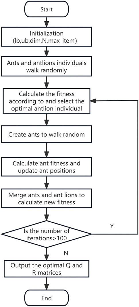
Figure 3. Alo algorithm flowchart.

2.3.3 Preview time optimization

To adapt to the need for certain predictability in direction control in actual driving and to reduce vehicle instability caused by repeated adjustments of the front wheel steering angle due to control response delays, this paper employs preview control technology to optimize steering response. Based on the current vehicle state, the kinematic model of the preview point is as Equation 22:

$\left\{\begin{array}{l}{\mathit{X}}_{\mathit{p}\mathit{r}\mathit{e}}=\mathit{X}+\mathit{v}\mathit{T}\mathit{cos}\left(\mathit{\psi }\right)\\ {\mathit{Y}}_{\mathit{p}\mathit{r}\mathit{e}}=\mathit{Y}+\mathit{v}\mathit{T}\mathit{sin}\left(\mathit{\psi }\right)\\ {\mathit{\psi }}_{\mathit{p}\mathit{r}\mathit{e}}=\mathit{\psi }+\mathit{\omega }\mathit{T}\end{array}\right.(22)$

where ${\mathit{X}}_{\mathit{p}\mathit{r}\mathit{e}}$ and ${\mathit{Y}}_{\mathit{p}\mathit{r}\mathit{e}}$ represents the coordinates of the preview point, and ${\mathit{\psi }}_{\mathit{p}\mathit{r}\mathit{e}}$ is the yaw angle of the preview point; $\mathit{X}$ and $\mathit{Y}$ denotes the position coordinates of the vehicle’s center of mass at the current time, $\mathit{\psi }$ and $\mathit{\omega }$ are the vehicle’s heading angle and yaw rate at the current moment, respectively, and $\mathit{v}$ is the vehicle’s speed.

The selection of the preview time $\mathit{T}$ is critical to the control performance. If $\mathit{T}$ is too small, the preview point distance is too short, which may lead to delayed control responses. Conversely, if $\mathit{T}$ is too large, the preview point distance is too far, which may result in significant deviations between the preview point and the actual path, thereby affecting system stability and response speed.

The simulation experiments method provided in reference (Cui et al., 2024) reveal the relationship between vehicle speed, road curvature, and preview time. The simulation results indicate that the selection of preview time is not only related to the magnitude of road curvature but also closely related to the trend of curvature changes. Taking a continuous lane-change scenario at 25 m/s as an example (see in Figure 4):

Figure 4

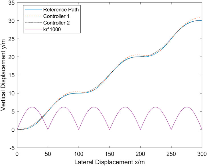
Figure 4. Tracking trajectories under two controllers.

When the curvature gradually increases, the second derivative of the path is positive, indicating that the vehicle is entering a sharper curve, with intensifying trajectory changes. Thus, the preview time needs to be shortened to improve response speed. When the curvature gradually decreases, the second derivative of the path is negative, indicating that the vehicle is entering a smoother road section where trajectory changes tend to stabilize. In this case, the preview time can be extended to achieve control over a longer distance.

Therefore, this paper proposes an adaptive preview time adjustment method based on fuzzy control, which dynamically optimizes the preview control parameters by comprehensively analyzing the vehicle speed, road curvature, and their variation characteristics. To reduce unnecessary calculation time, the controller is improved based on the rate of curvature change, adopting a hybrid control strategy that combines fixed preview time and dynamically adjusted preview time. Under the same simulation time of 15.5 s, 10 sets of the model’s actual runtime were collected for comparison. It was found that compared with the hybrid control strategy (see in Figure 5), the single fuzzy control not only has a longer runtime but also exhibits instability. In summary, the controller design considers the following key factors:

1. Vehicle speed: The preview time $\mathit{T}$ is positively correlated with the vehicle speed $\mathit{v}$. Under high-speed conditions, the preview distance needs to be extended to compensate for system response delays.

2. Road curvature: The curvature $\mathit{v}$ directly affects steering demands. On large-curvature road sections, the preview time needs to be increased. The rate of curvature change reflects the intensity of road morphology variations. When it exceeds a certain threshold, fuzzy dynamic adjustment is activated; otherwise, a fixed preview time is selected based solely on the current speed.

3. Second derivative of the road trajectory: When the second derivative of the reference trajectory is positive, a shorter preview time is required; when it is negative, a longer preview time is needed. Thus, the same controller cannot be used for both cases.

Figure 5

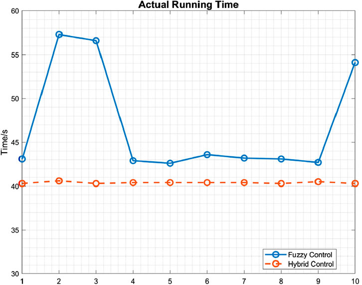
Figure 5. Simulink Model’s actual running time.

To achieve adaptive control, this paper first employs a fuzzy control algorithm with vehicle speed and road curvature as inputs. On straight or gently curved road sections, a fixed preview time is adopted; on sharp curves or under complex road conditions, the system automatically switches to fuzzy adjustment mode.

After extensive co-simulation testing using Carsim and Simulink, it was determined that excessive input variables could over-complicate the controller’s rule configuration. Therefore, this paper only categorizes based on the sign (positive or negative) of the second derivative of the reference trajectory. Based on the sign characteristics of the trajectory’s second derivative, differentiated control strategies are implemented, ultimately outputting an adaptive preview time $\mathit{T}$. This simplified design helps reduce the complexity of the fuzzy controller, thereby improving computational efficiency in practical applications. One single curvature point cannot reflect abrupt trajectory changes, and the vehicle may fail to respond in time during operation. Thus, this paper uses the rate of curvature change, denoted as $\mathit{K}\mathit{R}$, which is calculated by combining the curvature change rates from the current trajectory point $\mathit{d}\mathit{m}\mathit{i}\mathit{n}$ and the subsequent four points:

When $\mathit{K}\mathit{R}$ is less than the total number of points $\mathit{n}$, express as Equation 23:

$\mathit{K}\mathit{R}=\mathbf{1000}*\left(\mathit{k}\mathit{r}\left(\mathit{d}\mathit{m}\mathit{i}\mathit{n}\right)+\mathit{k}\mathit{r}\left(\mathit{d}\mathit{m}\mathit{i}\mathit{n}+\mathbf{1}\right)+\dots +\mathit{k}\mathit{r}\left(\mathit{d}\mathit{m}\mathit{i}\mathit{n}+\mathbf{4}\right)\right)(23)$

Otherwise, expressed as Equation 24:

$\mathit{K}\mathit{R}=\mathbf{1000}*\left(\mathit{k}\mathit{r}\left(\mathit{d}\mathit{m}\mathit{i}\mathit{n}\right)+\dots +\mathit{k}\mathit{r}\left(\mathit{n}\right)\right)(24)$

When the rate of curvature change is greater than 0, Controller 1 is used for solution. If it exceeds the switching threshold ${\mathit{K}\mathit{R}}_{\mathit{t}\mathit{h}}$, the fuzzy controller is activated; otherwise, the minimum preview time of 0 is adopted. When the rate of curvature change is less than or equal to 0, Controller 2 is used for solution. If it exceeds ${\mathit{K}\mathit{R}}_{\mathit{t}\mathit{h}}$, the fuzzy controller is activated; otherwise, the preview time is linearly solved. Through multiple experiments, it is verified that the value of $\mathit{T}$ is related to speed $\mathit{v}$ and generally follows quadratic Equation 25:

$\mathit{T}=\mathbf{0.013}\mathit{v}{\prime }^{\mathbf{2}}+\mathbf{0.03}{\mathit{v}}^{\prime }+\mathbf{0.008}(25)$

In the equation $v^{\prime }=v/5$, the operation stops when the length of the operating path $\mathit{s}$ exceeds the length of the reference path $\mathit{S}$.

2.3.4 Parameter selection and design

The most important parameters of the controller are the fuzzy controller and the threshold; a detailed analysis of the selection of both will be conducted next.

2.3.4.1 Fuzzy controller

The fuzzy controller designed in this paper adopts a precision configuration of 7-level input and 11-level output to ensure control accuracy while avoiding excessive complexity in rules. The precision levels of the input variables $\mathbf{v}$ and ${\mathit{k}}_{\mathit{r}}$ and output variables $\mathit{T}$ are as follows:

$\begin{array}{rr}\mathit{v}& =\left\{\mathit{N}\mathit{B},\mathit{N}\mathit{M},\mathit{N}\mathit{S},\mathit{Z}\mathit{O},\mathit{P}\mathit{S},\mathit{P}\mathit{M},\mathit{P}\mathit{B}\right\}\\ {\mathit{k}}_{\mathit{r}}& =\left\{\mathit{N}\mathit{B},\mathit{N}\mathit{M},\mathit{N}\mathit{S},\mathit{Z}\mathit{O},\mathit{P}\mathit{S},\mathit{P}\mathit{M},\mathit{P}\mathit{B}\right\}\\ \mathit{T}& =\left\{\mathit{N}\mathit{V},\mathit{N}\mathit{L},\mathit{N}\mathit{B},\mathit{N}\mathit{M},\mathit{N}\mathit{S},\mathit{Z}\mathit{O},\mathit{P}\mathit{S},\mathit{P}\mathit{M},\mathit{P}\mathit{B},\mathit{P}\mathit{L},\mathit{P}\mathit{V}\right\}\end{array}$

The universe of discourse for vehicle speed $\mathbf{v}$ is set to [0, 30] m/s, which covers the range from vehicle standstill to high-speed driving and ensures the threshold can adapt to multiple scenarios such as low-speed urban driving, medium-speed suburban driving, and high-speed highway driving. The universe of discourse for road curvature ${\mathit{k}}_{\mathit{r}}$ is set to [0, 0.02] ${\mathit{m}}^{-\mathbf{1}}$; it includes the approximately zero curvature of straight road sections and also covers regular medium-curvature curves, preventing threshold failure caused by extreme curvature. The universe of discourse for preview time T is set to [0, 0.5] s, which aligns with the typical control cycle range of vehicles to ensure threshold update efficiency.

Input variables adopt the Gauss2 membership function to achieve smooth transition, while output variables use the Trimf membership function to ensure defuzzification accuracy. The design of fuzzy rules starts with a rough draft based on prior experience, which is then adjusted through iterative upward and downward tuning, and finally validated via simulation to determine the optimal set of rules. The membership functions of each input and output variable are shown in Figure 6. The fuzzy rules for the two controllers are listed in Table 1. When the second derivative of the trajectory is greater than zero, Fuzzy Rule 1 is applied; when the second derivative of the trajectory is less than or equal to zero, Fuzzy Rule 2 is applied. The inference results of the two fuzzy controllers are illustrated in Figure 7.

Figure 6

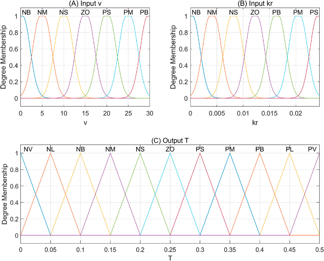
Figure 6. Membership Functions of (A) Inputs (v). (B) Inputs (kr) and (C) Output (T) with Fuzzy State Labels (NB, NM, NS, ZO, PS, PM, PB, NV, NL, PL, PV) and Axis Scale Labels.

Table 1

Table 1. Fuzzy rules.

Figure 7

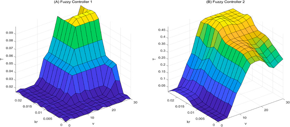
Figure 7. Fuzzy Inference Results of kr-v-T Relationship with Axis Variable Labels (kr, v, T) and Scale Labels. (A) Fuzzy Controller 1. (B) Fuzzy Controller 2.

2.3.4.2 Switching threshold filte

The selection of the switching threshold ${\mathit{K}\mathit{R}}_{\mathit{t}\mathit{h}}$ is critical in the optimization of preview time T, as it fundamentally determines whether adaptive adjustment of preview time can be achieved, thereby governing the overall control performance of the system.

Excessively low ${\mathit{K}\mathit{R}}_{\mathit{t}\mathit{h}}$ triggers premature fuzzy controller activation during allowable trajectory perturbations. The associated computation latency from frequent switching impedes rapid steady-state attainment, counteracting response time reduction while increasing power dissipation through repeated initialization. Conversely, excessive ${\mathit{K}\mathit{R}}_{\mathit{t}\mathit{h}}$ values diminish trajectory variation sensitivity, compromising system adaptability. This suppresses preview time adjustment, fixing T within a static operational envelope rather than enabling real-time optimization. Such insufficient performance contradicts the core objective. To address this scenario, this study initially selects five candidate threshold values: 1, 1.5, 2, 2.5, and 3, followed by designed experiments for subsequent screening.

The S-path comprises straight trajectories, curved trajectories, and the transitions between them, making it suitable for verifying the tracking performance of turning paths. So the experimental procedure chooses tracking the S-shaped trajectory illustrated in Figure 8A at three speeds—10 m/s (low speed), 20 m/s (medium speed), and 25 m/s (high speed)—under five distinct states. Subsequently, calculating fitness values to evaluate model performance in terms of tracking accuracy and stability. The distance deviation, steering angle error, and output steering angle are discretized to obtain $e_d\left(i\right)$, $e_{\phi }\left(i\right)$, and $\mathrm{\delta }\left(\mathrm{i}\right)$, the fitness function is defined as Equation 26:

$\mathit{J}=\Delta \mathit{t}{\displaystyle \sum _{\mathit{i}=\mathbf{1}}^{\mathit{n}}}\left({\mathit{\omega }}_{\mathbf{1}}\left|{\mathit{e}}_{\mathit{d}}\left(\mathit{i}\right)\right|+{\mathit{\omega }}_{\mathbf{2}}\left|{\mathit{e}}_{\mathit{\phi }}\left(\mathit{i}\right)|+{\mathit{\omega }}_{\mathbf{3}}\right|\mathit{\delta }\left.\left(\mathit{i}\right)\right|\right)(26)$

where ${\mathit{\omega }}_{\mathbf{1}}$, ${\mathit{\omega }}_{\mathbf{2}}$, and ${\mathit{\omega }}_{\mathbf{3}}$ represent the weighting coefficients for the three variables respectively, and $\Delta \mathrm{t}$ denotes the sampling time interval. The fitness values are normalized, and a line chart as shown in Figure 8B is plotted. After comprehensive consideration, three levels (1.5, 2, and 2.5) are selected for further research.

Figure 8

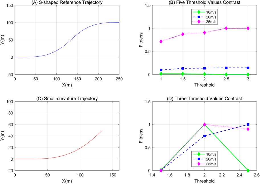
Figure 8. Threshold Filtering Experiment Results with Axis Labels (X, Y, Threshold, Fitness), Vehicle Speed Labels (10m/s, 20m/s, 25m/s) and Curve Color Labels. (A) S-shaped Reference Trajectory. (B) Five Threshold Values Contrast. (C) Small-curvature Trajectory. (D) Three Threshold Values Contrast.

A comparative analysis of the three thresholds was conducted under conditions of low road adhesion (with $\mathrm{\mu }=0.6$) to evaluate the robustness of the model in harsh environments. For the small-curvature trajectory as shown in Figure 8C, it is primarily designed to verify the tracking performance and stability specifically under the scenario of small curvature combined with high speed. The fitness status is presented in Figure 8D.

After a comprehensive assessment of tracking accuracy and stability, this paper adopts 1.5 as the threshold for subsequent studies. Otherwise, for the output steering angle δ, which directly determines the direction of the vehicle’s steering and the responsiveness of trajectory adjustment to ensure the vehicle maintains good operational stability across diverse driving conditions, strict range constraints on the front-wheel angle are essential. This prevents over steering, yaw rate from exceeding the safety threshold, and the subsequent risks of vehicle trajectory deviation or loss of body attitude control, with the front-wheel angle specifically limited to a range of $\left[-0.5,0.5\right]$. The complete flowchart of the controller is finally obtained, as shown in Figure 9.

Figure 9

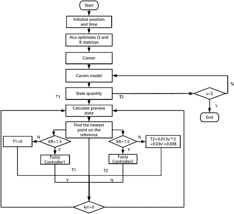
Figure 9. Controller flowchart.

3 Ethics statement

3.1 Data and copyright compliance

All simulation data used in this study were generated through the established 2-DOF vehicle dynamics model and improved LQR control algorithm. No third-party private datasets or copyrighted materials were used without permission. For cited literature and public domain references, have strictly followed academic citation norms to ensure compliance with copyright laws.

3.2 Conflict of interest

All authors declare no competing financial interests or personal relationships that could have influenced the design of the study, analysis of data, or writing of the manuscript.

3.3 Publishing ethics

This manuscript is original, has not been published previously, and is not under consideration for publication in any other journal. All authors have read and approved the final version of the manuscript, and confirm that no essential content has been omitted or misrepresented.

4 Results

To validate the effectiveness of the designed controller, a test environment is built based on the CarSim/Simulink co-simulation platform, and the following comparative experiments are conducted:

1. Classical LQR controller (without preview, and with fixed weights: $\mathbf{Q}=\mathbf{\text{diag}}\left[\mathbf{1},\mathbf{1},\mathbf{1},\mathbf{1}\right]$, $\mathbf{R}=\mathbf{10}$);

2. Fixed preview time of 0.1 s, with weight optimization for the LQR algorithm using the ALO;

3. Fuzzy algorithm-optimized preview time combined with the ALO algorithm to optimize the weights;

The tracking results of the three controllers under the same reference path are compared and analyzed. Two typical extreme scenarios—Double Lane Change and Double Sine—are selected as reference trajectories. Control performance is comprehensively through three indicators:distance deviation ${\mathit{e}}_{\mathit{d}}$, yaw rate $\dot{\mathit{\psi }}$, and side slip angle $\mathit{\beta }$.

1. Distance deviation ${\mathit{e}}_{\mathit{d}}$: The linear distance between the current vehicle position and the nearest point on the reference trajectory, which directly reflects the steady-state accuracy of the control system and the effectiveness of the front wheel angle control quantity.

2. Yaw rate $\dot{\mathit{\psi }}$: The rotational angular velocity of the vehicle around its vertical axis, reflecting the controller’s ability to track the desired yaw moment and stability during abrupt changes in lateral acceleration.

3. Side slip angle $\mathit{\beta }$: The angle between the vehicle’s velocity direction and its longitudinal axis of the vehicle, directly characterizing the dynamic stability of the vehicle.

To thoroughly validate the performance of the designed controller, in the co-simulation experiments, the vehicle speed under the two different working conditions is set to a constant value without special speed planning. Considering the vehicle driving safety and controller performance under different speeds, two vehicle speeds are configured: 15 m/s represents medium-high speed, which is used to test the stability and accuracy of the controller at lower speeds; 25 m/s represents relatively high speed, which is used to test the fast response and trajectory accuracy of the controller, so as to more comprehensively evaluate the performance of the controller under various working conditions. The experimental simulation step size is 0.05 s, and key dynamic parameters of the test vehicle and the simulation environment are listed in Table 2:

Table 2

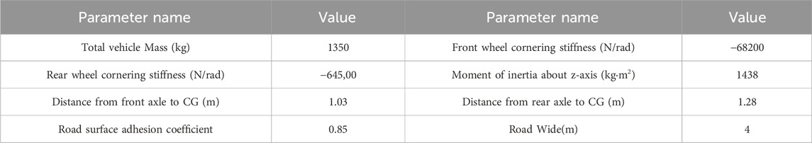
Table 2. Vehicle parameters table.

4.1 Simulation scenario 1

The double lane change scenario requires the control algorithm to respond rapidly to environmental changes, providing a comprehensive test of the control system’s adaptability to time-varying curvature. It is well-suited for evaluating the real-time optimization performance of the controller. The trajectory equation is defined as Equation 27:

$\mathit{Y}\left(\mathit{X}\right)=\frac{\mathit{c}}{\mathbf{2}\mathit{\pi }}\left\{\mathit{\pi }+\frac{\mathbf{2}\mathit{\pi }}{\mathit{d}}\left(\mathit{X}-\frac{\mathit{d}}{\mathbf{2}}\right)+\mathit{sin}\left[\frac{\mathbf{2}\mathit{\pi }}{\mathit{d}}\left(\mathit{X}-\frac{\mathit{d}}{\mathbf{2}}\right)\right]\right\}(27)$

where, $\mathrm{c}=10$, $\mathrm{d}=100$. The tracking results under this scenario are shown in Figures 10, 11:

Figure 10

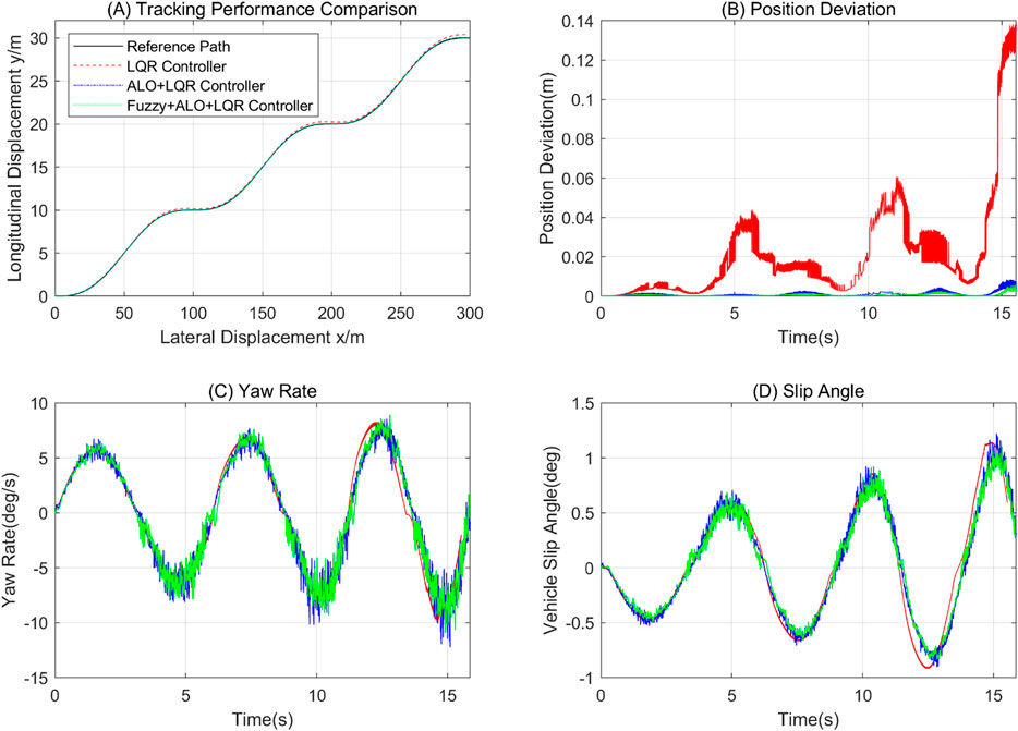
Figure 10. Controller Performance Comparison under 15m/s Double Lane Change Scenario with Axis Labels (Tracking performance Comparison (A) Lateral Displacement, (B) Position Deviation, (C) Yaw Rate, (D) Slip Angle, Time) and Controller Type Labels ( Reference Path, LQR, ALO+LQR, Fuzzy+ALO+LQR).

Figure 11

Figure 11. Controller Performance Comparison under 25m/s Double Lane Change Scenario with Axis Labels (Tracking performance Comparison (A) Lateral Displacement, (B) Position Deviation, (C) Yaw Rate, (D) Slip Angle, Time) and Controller Type Labels (Reference Path, LQR, ALO+LQR, Fuzzy+ALO+LQR).

4.2 Simulation Scenario 2

The double sine trajectory requires the vehicle to complete two directional switches within a short time, making it suitable for testing the controller’s dynamic response speed, yaw stability, and yaw rate. It is ideal for high-precision and high-stability validation. The specific equation is as Equation 28:

$\mathit{Y}\left(\mathit{X}\right)=\frac{{\mathit{d}}_{\mathit{y}\mathbf{1}}}{\mathbf{2}}\left(\mathbf{1}+\mathit{tanh}\left({\mathit{z}}_{\mathbf{1}}\right)\right)-\frac{{\mathit{d}}_{\mathit{y}\mathbf{2}}}{\mathbf{2}}\left(\mathbf{1}+\mathit{tanh}\left({\mathit{z}}_{\mathbf{2}}\right)\right)(28)$

Where ${\mathit{d}}_{\mathit{y}\mathbf{1}}=\mathbf{4.05}$, ${\mathit{d}}_{\mathit{y}\mathbf{2}}=\mathbf{5.7}$, ${\mathit{z}}_{\mathbf{1}}=\frac{\mathbf{2.4}}{\mathbf{25}}\left(\mathit{X}-\mathbf{27.19}\right)-\mathbf{1.2}$, ${\mathit{z}}_{\mathbf{2}}=\frac{\mathbf{2.4}}{\mathbf{21.95}}\left(\mathit{X}-\mathbf{56.46}\right)-\mathbf{1.2}$, is the horizontal coordinate of the trajectory. The tracking results under this scenario are shown in Figures 12, 13.

Figure 12

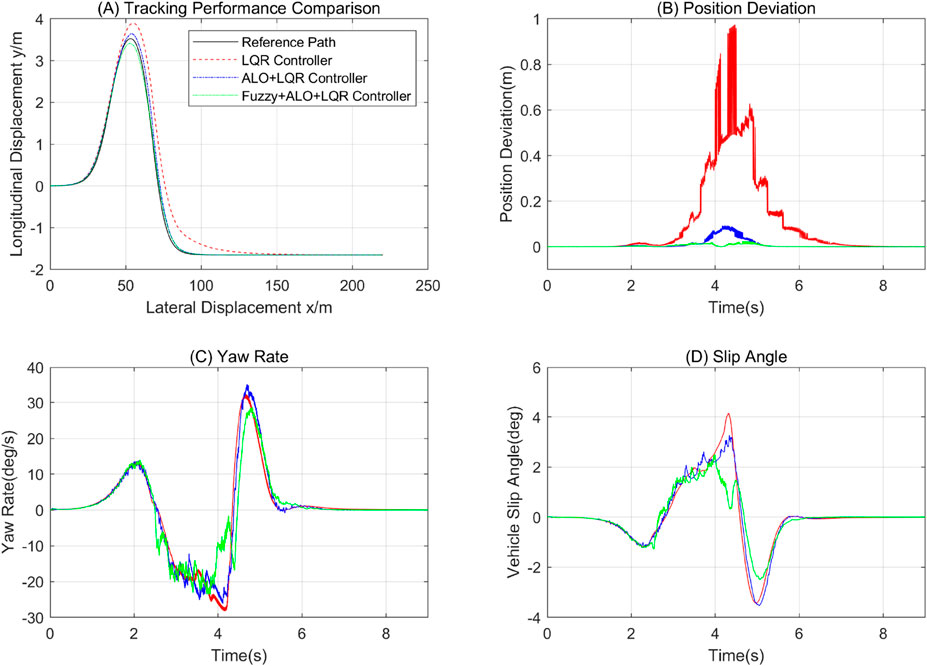
Figure 12. Controller Performance Analysis under 15m/s Double Sine Trajectory Scenario with Axis Labels (Tracking performance Comparison (A) Lateral Displacement, (B) Position Deviation, (C) Yaw Rate, (D) Slip Angle, Time) and Controller Type Labels (Reference Path, LQR, ALO+LQR, Fuzzy+ALO+LQR).

Figure 13

Figure 13. Dynamic Control Strategy Comparison under 25m/s Double Sine Trajectory Scenario with Axis Labels (Tracking performance Comparison (A) Lateral Displacement, (B) Position Deviation, (C) Yaw Rate, (D) Slip Angle, Time) and Controller Type Labels (Reference Path, LQR, ALO+LQR, Fuzzy+ALO+LQR).

4.3 Simulation results analysis

As clearly illustrated, the LQR + ALO + Fuzzy controller designed in this paper achieves varying degrees of optimization in three key aspects: distance deviation, yaw rate, and slip angle. The maximum absolute values and average values of these three metrics are summarized in Tables 3, 4 as follows:

Table 3

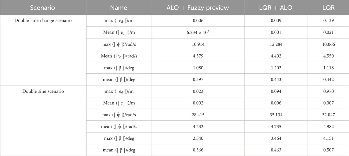
Table 3. Double lane change and double sine scenarios at 15 m/s.

Table 4

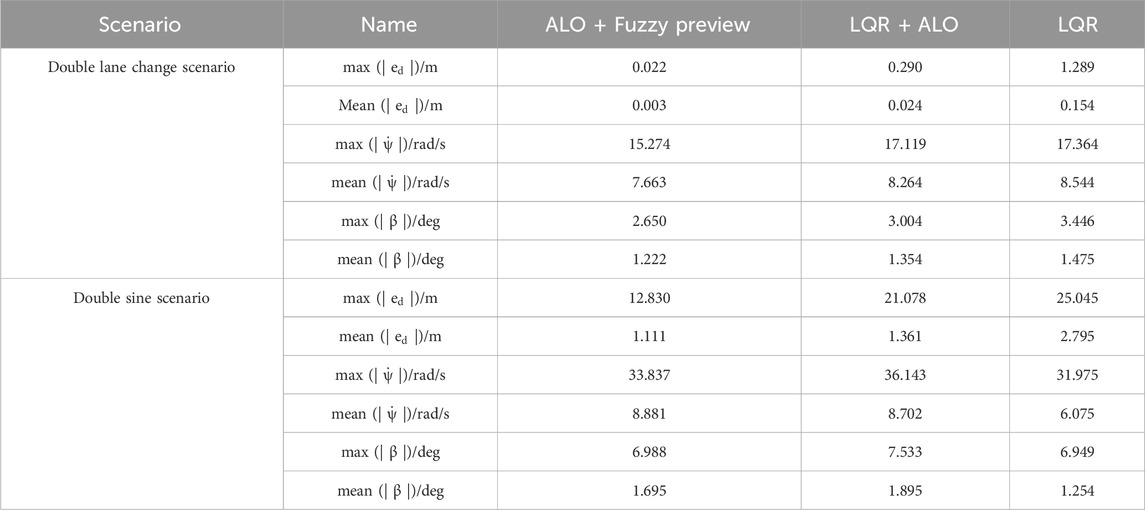
Table 4. Double lane change and double sine scenarios at 25 m/s.

In the performance evaluation of vehicle path tracking control, the composite control strategy incorporating fuzzy algorithms demonstrates significant advantages. Under the 15 m/s double lane change scenario, the maximum lateral position error of this strategy is as low as 0.006 m, which is only 66.67% of that of the LQR + ALO strategy and represents a 95.66% reduction compared to the traditional LQR strategy. In the double sine scenario, the maximum distance deviation of LQR + ALO + Fuzzy is reduced by 75.53% compared to the ALO + LQR strategy, indicating its excellent adaptability to paths with abrupt curvature changes. Although the performance of the improved controller slightly declines under high-speed conditions, its accuracy in high-speed scenarios still far surpasses that of traditional methods. For example, in the 25 m/s double lane change scenario, its average error is only 12.5% of that of ALO + LQR; in the 25 m/s double sine scenario, its average distance deviation is only 39.74% of that of the traditional LQR controller. These results not only highlight the high tracking precision of the improved strategy in high-speed dynamic scenarios but also expose the limitations of traditional LQR and ALO + LQR strategies in balancing stability and accuracy at high speeds.

In terms of vehicle dynamic response, the time-varying controller quickly adapts to road conditions through rapid adjustments. In the 15 m/s double lane change scenario, its yaw rate shows minimal difference compared to traditional controllers, but its average steering angular velocity is lower than that of the LQR controller. In the 15 m/s double sine scenario, the maximum yaw rate of LQR + ALO + Fuzzy is reduced by 11.33% compared to traditional LQR, and the average value is optimized by 15.59%, validating the effectiveness of variable preview time control in suppressing steering oscillations. Under the 25 m/s high-speed scenario, this strategy reduces the maximum yaw rate by 10.78% compared to LQR + ALO in the double lane change scenario, demonstrating the synergistic effect of fuzzy control and ALO optimization in enhancing steering smoothness. However, in the double sine scenario, although the maximum yaw rate is reduced by 6.38% compared to ALO + LQR, the average value slightly increases, indicating that oscillations may intensify under high-speed conditions with abrupt curvature changes.

Regarding vehicle stability, the LQR + ALO + Fuzzy strategy significantly enhances the anti-slip capability. Under the 15 m/s continuous lane-change maneuver, its slip angle is 1.080°; the maximum value is 10.15% lower than that of the ALO + LQR strategy, and the average value is optimized by 10.38%. Under the 15 m/s double-lane-change maneuver, the maximum value of its slip angle is 26.67% lower than that of the ALO + LQR strategy, and the average value is 20.95% lower. In the 25 m/s high-speed continuous lane-change maneuver, the maximum value of its slip angle is 11.79% smaller than that of the LQR + ALO strategy before the integration of fuzzy control, and the average value is 9.75% smaller. Notably, under the 25 m/s double-lane-change maneuver, the average slip angles of both the ALO improved and Fuzzy + ALO improved strategies are higher than that of the traditional LQR; however, this increase is suppressed after the introduction of the improved preview time: compared with the Fuzzy + ALO strategy before fuzzy optimization, the LQR + ALO + Fuzzy strategy achieves a 7.24% reduction in the maximum value and a 10.56% reduction in the average value. This fully indicates that although the performance of the designed controller in some indicators under high-speed conditions is slightly degraded compared with that under medium and low-speed conditions, it still has significant advantages in terms of high-speed stability compared with the traditional controller with fixed preview time.

5 Conclusion

5.1 Contribution of the article

1. Addressing the core limitation of fixed-weight LQR controllers. To tackle the poor adaptability of fixed-weight LQR controllers to complex road conditions and curvature changes, this study introduces the ALO algorithm to solve for the optimal coefficient matrices of the LQR controller under different path conditions. By dynamically optimizing based on specific path characteristics, the controller’s adaptability to various trajectory forms is significantly enhanced.

2. Proposing a hybrid strategy to overcome the limitation of fixed preview time Aiming at the defect that fixed preview time in traditional preview control cannot adapt to diverse road scenarios, this study puts forward a hybrid control strategy. This strategy takes dynamic adjustment of preview time as its basic framework and further classifies and optimizes different curvature change rates and reference path change rates. Such multi-dimensional adjustment ensures that preview control can more accurately match real-time road conditions, avoiding control response delays or overshoot caused by fixed preview time.

3. Verifying performance and practical value through simulations Simulation results confirm the effectiveness of the designed controller. It can not only effectively adapt to dynamic changes in path conditions, such as sudden increases in curvature or complex trajectory switches, but also improve the path-tracking accuracy during vehicle operation while ensuring driving stability.

5.2 Limitations of controller

However, the proposed controller exhibits significant limitations under high-speed conditions. Although it can maintain the vehicle within the scope of basic stability requirements while ensuring tracking accuracy, it still sacrifices partial dynamic stability, which is specifically manifested in an increase in yaw rate. This indicates that the current control strategy cannot meet the strict stability requirements for high-speed driving, mainly due to two key factors: first, the linearization of the 2-DOF vehicle model ignores nonlinear dynamic characteristics such as tire load transfer and tire slip angle saturation at high speeds, leading to deviations between the control model and the actual vehicle state; second, the fuzzy preview controller adopts a simplified rule design, which fails to fully capture the complex coupling relationship between high-speed vehicle dynamics and path characteristics, resulting in sub-optimal preview time adjustment.

5.3 Outlook

Future research will address the aforementioned limitations from three aspects: Firstly, increase the degree of freedom of the nonlinear vehicle dynamics model and improve the similarity between the linearized model and the actual model. Secondly, the fuzzy preview control rules will be optimized by adding input parameters such as lateral acceleration, to improve the adaptability of the preview strategy to high-speed and extreme curvature scenarios. Third, real-vehicle validation experiments will be conducted to verify the controller’s performance under real road conditions, and further calibrate the control parameters to narrow the gap between simulation results and practical applications.

Data availability statement

The raw data supporting the conclusions of this article will be made available by the authors, without undue reservation.

Author contributions

LYa: Conceptualization, Investigation, Methodology, Software, Writing – original draft, Writing – review and editing. GX: Funding acquisition, Supervision, Writing – review and editing. LYu: Data curation, Validation, Writing – original draft. LZ: Formal Analysis, Visualization, Writing – review and editing.

Funding

The authors declare that financial support was received for the research and/or publication of this article. Ministry of Education 2024 Industry-University Cooperation Collaborative Education Project (CX20241206). This work was partially funded by the Ministry of Education 2024 Industry-University Cooperation Collaborative Education Project (Grant No. CX20241206), which made the research possible.

Acknowledgements

The authors would like to express sincere gratitude to all colleagues who contributed to this work. Special thanks go to Liang, Y.X., Liu, Z.H. for their valuable suggestions on experimental design and careful review of the manuscript. We also acknowledge the support from College of Electrical Engineering and New Energy, China Three Gorges University for providing experimental facilities and research platforms. Finally, we appreciate the constructive comments and suggestions from the reviewers, which greatly improved the quality of this manuscript.

Conflict of interest

The authors declare that the research was conducted in the absence of any commercial or financial relationships that could be construed as a potential conflict of interest.

Generative AI statement

The authors declare that no Generative AI was used in the creation of this manuscript.

Any alternative text (alt text) provided alongside figures in this article has been generated by Frontiers with the support of artificial intelligence and reasonable efforts have been made to ensure accuracy, including review by the authors wherever possible. If you identify any issues, please contact us.

Publisher’s note

All claims expressed in this article are solely those of the authors and do not necessarily represent those of their affiliated organizations, or those of the publisher, the editors and the reviewers. Any product that may be evaluated in this article, or claim that may be made by its manufacturer, is not guaranteed or endorsed by the publisher.

References

Chen, W. W., Wang, J. E., Wang, M. L., and Wang, J. B. (2014). Adaptive preview control for lateral motion of vision-guided intelligent vehicles. China Mech. Eng. 25 (5), 698–704. doi:10.3969/j.issn.1004-132X.2014.05.023

CrossRef Full Text | Google Scholar

Cui, M. Y., Huang, H. Y., Xu, Q., Wang, J. Q., Sekiguchi, T., and Geng, L. (2022). Key technologies of architecture, function and application for intelligent connected vehicles. J. Tsinghua Univ. Sci. Technol. 62 (3), 493–508. doi:10.16511/j.cnki.qhdxxb.2021.26.026

CrossRef Full Text | Google Scholar

Cui, K. C., Gao, S., Wang, P. W., Zhou, H. H., and Zhang, Y. L. (2024). Intelligent vehicle tracking controller design based on feedforward + prediction LQR. Sci. Technol. Eng. 24 (10), 4287–4299. doi:10.12404/j.issn.1671-1815.2303956

CrossRef Full Text | Google Scholar

Gong, H. H., He, D. L., He, H., Du, J., and Dong, M. X. (2023). Suppression of load sway in overhead cranes using linear quadratic regulator based on genetic algorithm. Hoisting Conveying Mach. (17), 66–72. Available online at: https://kns.cnki.net/kcms2/article/abstract?v=kg5wHjgO96XnbhEA_lqD7JTkTdEi92zEvSa3iUZBwEcM1b18yg2WH3TKmABwlRbf04yZB7dcHK1Fwbo6fg06M0zQyIcYrSurfNwlnBykBS3gvpLE5WpTU7PJLC9gAnmeqLJ88Kc0YTEl0C0ymTbZ0FbLw64ij0Q3KDUCfFqPuXwlTanaVPRslkG6zbc4DE.

Google Scholar

Guo, H. Y., Cao, D. P., Chen, H., Sun, Z. P., and Hu, Y. F. (2019). Model predictive path following control for autonomous cars considering a measurable disturbance: implementation, testing, and verification. Mech. Syst. Signal Process. 118, 41–60. doi:10.1016/j.ymssp.2018.08.028

CrossRef Full Text | Google Scholar

Hu, C., Gao, H. B., Guo, J. H., Taghavifar, H., Qin, Y. C., and Na, J. (2021). RISE-Based integrated motion control of autonomous ground vehicles with asymptotic prescribed performance. IEEE Trans. Syst. Man, Cybern. Syst. 51 (9), 5336–5348. doi:10.1109/TSMC.2019.2950468

CrossRef Full Text | Google Scholar

Hu, J., Zhong, X. K., Chen, R. N., Zhu, L. L., Xu, W. C., and Zhang, M. C. (2022). Path tracking control of intelligent vehicles based on fuzzy LQR. Automot. Eng. 44 (1), 17–25+43. doi:10.19562/j.chinasae.qcgc.2022.01.003

CrossRef Full Text | Google Scholar

Ibrahim, A. E. B. (2022). Self-tuning look-ahead distance of pure-pursuit path-following control for autonomous vehicles using an automated curve information extraction method. Int. J. Intelligent Transp. Syst. Res. 20 (3), 709–719. doi:10.1007/s13177-022-00319-z

CrossRef Full Text | Google Scholar

Kaleemullah, M., and Faris, W. F. (2022). Optimisation of robust and LQR control parameters for discrete car model using genetic algorithm. Int. J. Veh. Syst. Model. Test. 16 (1), 40–63. doi:10.1504/ijvsmt.2022.126968

CrossRef Full Text | Google Scholar

Li, J. T., and Chen, Z. J. (2024). Nonlinear model predictive control path tracking based on adaptive path preview. J. Tongji Univ. Nat. Sci. 52 (S1), 158–164. doi:10.11908/j.issn.0253-374x.24723

CrossRef Full Text | Google Scholar

Li, Y. N., Wan, Y., Liang, X. C., and Hou, J. R. (2024). “LQR lateral control with variable preview distance for security inspection robots,” in Techniques of automation and applications, 1–9. Available online at: https://link.cnki.net/urlid/23.1474.TP.20241218.1102.032.

Google Scholar

Norouzi, A., Heidarifar, H., Borhan, H., Shahbakhti, M., and Koch, C. R. (2023). Integrating Machine Learning and Model Predictive Control for automotive applications: a review and future directions. A Rev. future Dir. Eng. Appl. Artif. Intell. 120, 105878. doi:10.1016/j.engappai.2023.105878

CrossRef Full Text | Google Scholar

Ribeiro, A. M., Fioravanti, A. R., Moutinho, A., and de Paiva, E. C. (2020). Nonlinear state-feedback design for vehicle lateral control using sum-of-squares programming. Veh. Syst. Dyn. 60 (3), 743–769. doi:10.1080/00423114.2020.1844905

CrossRef Full Text | Google Scholar

Shi, Q., Zhang, J. L., and Yang, M. (2021). Curvature adaptive control based path following for automatic driving vehicles in private area. J. Shanghai Jiaot. Univ. Sci. 26 (5), 690–698. doi:10.1007/s12204-021-2359-4

CrossRef Full Text | Google Scholar

Wang, Y., Chen, Q. Z., Gao, L. L., Zhang, W. J., and Wang, S. (2020). Path tracking method for distributed drive vehicles based on predictive-fuzzy joint control. Sci. Technol. Eng. 20 (36), 15100–15108.

Google Scholar

Wang, B. L., Li, Y. W., Zhao, Y., Song, S., and Wang, Y. Q. (2023). Lateral tracking control strategy of LQR optimized by ant lion optimizer. J. Chongqing Univ. Technol. Nat. Sci. 37 (4), 27–38. doi:10.3969/j.issn.1674-8425(z).2023.04.004

CrossRef Full Text | Google Scholar

Wang, X. G., Wu, W. L., and He, W. (2024a). Research on lateral and longitudinal tracking control of vehicles with LQR based on PSO. Automation and Instrum. 39 (10), 136–142. doi:10.19557/j.cnki.1001-9944.2024.10.029

CrossRef Full Text | Google Scholar

Wang, F. A., Wang, B. Y., Zhang, Z. G., Xie, K. T., Li, A. N., Ni, C., et al. (2024b). Adaptive preview tracking fuzzy control algorithm for tracked vehicles. Trans. Chin. Soc. Agric. Eng. 40 (10), 32–43. doi:10.11975/j.issn.1002-6819.202401039

CrossRef Full Text | Google Scholar

Zhang, J. H., Chen, D. P., and Li, Q. (2020). Research status and development trend of automatic driving technology. Sci. Technol. Eng. 20 (09), 3394–3403. Available online at: https://kns.cnki.net/kcms2/article/abstract?v=kg5wHjgO96VGm8PN0ztNHsjgX08Cw98ftvtABw6ivHQsdFNCPTSRu7PTkq4RnzAUe1CBNP0g5k8XiEUg1jRlD2UqJrKDLUJus5LbPwG1DWS8p8zRzv8G75VgEbXUi49SLg3iGwWQPBePphNZjnfoZ1J0tH561olZVr0OdDXIwfhHX8SmasTnb714n2kl&uniplatform=NZKPT&language=CHS.

Google Scholar

Zhang, D., Liu, H., Jiao, X., and Zhang, T. (2024). “MPC-based trajectory tracking control strategy incorporating autonomous lane-changing mechanism for intelligent vehicles,” in In proceedings of the 2024 8th CAA international conference on vehicular control and intelligence (CVCI) (Chongqing, China: IEEE), 1–6. doi:10.1109/CVCI63518.2024.10830218

CrossRef Full Text | Google Scholar

Zhou, J. W., Wen, J. H., Yao, L. W., Yang, Z. D., Xu, L. J., and Yao, L. J. (2025). Agricultural machinery path tracking with varying curvatures based on an improved pure-pursuit method. Agriculture 15 (3), 266. doi:10.3390/agriculture15030266

CrossRef Full Text | Google Scholar