Abstract
Agricultural water is an important source of foodborne pathogens on produce farms. Managing water-associated risks does not lend itself to one-size-fits-all approaches due to the heterogeneous nature of freshwater environments. To improve our ability to develop location-specific risk management practices, a study was conducted in two produce-growing regions to (i) characterize the relationship between Escherichia coli levels and pathogen presence in agricultural water, and (ii) identify environmental factors associated with pathogen detection. Three AZ and six NY waterways were sampled longitudinally using 10-L grab samples (GS) and 24-h Moore swabs (MS). Regression showed that the likelihood of Salmonella detection (Odds Ratio [OR] = 2.18), and eaeA-stx codetection (OR = 6.49) was significantly greater for MS compared to GS, while the likelihood of detecting L. monocytogenes was not. Regression also showed that eaeA-stx codetection in AZ (OR = 50.2) and NY (OR = 18.4), and Salmonella detection in AZ (OR = 4.4) were significantly associated with E. coli levels, while Salmonella detection in NY was not. Random forest analysis indicated that interactions between environmental factors (e.g., rainfall, temperature, turbidity) (i) were associated with likelihood of pathogen detection and (ii) mediated the relationship between E. coli levels and likelihood of pathogen detection. Our findings suggest that (i) environmental heterogeneity, including interactions between factors, affects microbial water quality, and (ii) E. coli levels alone may not be a suitable indicator of food safety risks. Instead, targeted methods that utilize environmental and microbial data (e.g., models that use turbidity and E. coli levels to predict when there is a high or low risk of surface water being contaminated by pathogens) are needed to assess and mitigate the food safety risks associated with preharvest water use. By identifying environmental factors associated with an increased likelihood of detecting pathogens in agricultural water, this study provides information that (i) can be used to assess when pathogen contamination of agricultural water is likely to occur, and (ii) facilitate development of targeted interventions for individual water sources, providing an alternative to existing one-size-fits-all approaches.
Introduction
Preharvest surface water use for produce production (e.g., irrigation, fertigation, pesticide application, dust abatement) has been repeatedly identified as a factor associated with an increased likelihood of foodborne pathogen contamination of produce (e.g., Mody et al., 2011; Strawn et al., 2013b; Holvoet et al., 2014; Weller et al., 2015b). This is largely because (i) surface water can act as a source (Micallef et al., 2012; McEgan et al., 2013a) and transmission pathway (Girardin et al., 2005; Mody et al., 2011; Weller et al., 2015b) for foodborne pathogens in farm environments and (ii) the use of pathogen-contaminated water can transfer pathogens to produce directly (Guan et al., 2001; Erickson et al., 2010) and indirectly [e.g., through contamination of the farm environment (Ibenyassine et al., 2006; Oliveira et al., 2012)]. In fact, irrigation with untreated surface water has been repeatedly associated with the isolation of foodborne pathogens from preharvest environments (Guan et al., 2001; Strawn et al., 2013b; Holvoet et al., 2014; Weller et al., 2015b), and identified as a potential cause of outbreaks linked to produce (Mody et al., 2011; Baloch, 2014; Centers for Disease Control and Prevention (U.S.), 2018; Food and Drug Administration (U.S.), 2018). Thus, mitigating the food safety risks associated with preharvest surface water use is a priority. Indeed, the US Food and Drug Administration proposed microbial water quality standards as part of the Food Safety Modernization Act’s (FSMA) Produce Safety Rule. However, understanding and complying with the proposed standard while ensuring water availability has been cited in industry magazines and grower surveys as a challenge facing growers (Alexander, 2015; Dery et al., 2019; Wall et al., 2019). For example, interpretation of E. coli test results is complicated by temporal variation in microbial water quality (Goyal et al., 1977; Hipsey et al., 2008; Payment and Locas, 2011; Pandey et al., 2012). Since the samples used to determine if a water source meets the proposed standard can be collected up to 4 years before the water source is used for produce production, meeting the standard also may be a poor approximation of water quality at time of use (Havelaar et al., 2017; Truitt et al., 2018). Acceptance of E. coli-based water standards is further complicated by conflicting data on the relationship between E. coli levels and pathogen presence in the literature (Harwood et al., 2005; Wilkes et al., 2009; Benjamin et al., 2013; Economou et al., 2013; McEgan et al., 2013a; Pachepsky et al., 2015). While some studies argue that high E. coli levels are associated with an increased likelihood of detecting pathogens in agricultural water (Edberg et al., 2000; Wilkes et al., 2009; Payment and Locas, 2011), other studies disagree (Harwood et al., 2005; Benjamin et al., 2013; Pachepsky et al., 2015; Antaki et al., 2016). While this differentiation is often not made, these observations are consistent with the fact that E. coli is considered an indicator of potential fecal contamination, and not an “index organism” [detection of an index organism suggests the presence of an ecologically similar or closely related pathogen (Busta et al., 2006; Chapin et al., 2014)]. Despite this, it is important to understand the relationship between E. coli levels and foodborne pathogen contamination of agricultural water since data on E. coli levels are used to guide efforts to mitigate the microbial food safety risks associated with preharvest surface water use (e.g., to decide if and when corrective measures such as water treatment should be implemented). Thus, data on the relationship between E. coli levels and foodborne pathogen contamination of agricultural water are essential for identifying when and where E. coli levels can be used (alone or in conjunction with other data) to manage the food safety risks associated with preharvest water use. Promising alternative approaches include models that predict likelihood of pathogen presence at specific times and sampling locations along a waterway using a variety of spatially and/or temporally explicit data. However, to develop these alternative approaches additional data on factors (e.g., weather, physicochemical water quality) that drive variation in E. coli levels and pathogen presence in different regions is needed.
Like E. coli levels, the prevalence of key foodborne pathogens in surface water also varies between studies and over time. For example, 30 and 63% of surface water samples collected from New York produce farms in 2010 (Weller et al., 2015b) and 2015 (Weller et al., 2015a), respectively, were L. monocytogenes-positive. Similarly, 29% (Kayed, 2004), 58% (Ijabadeniyi et al., 2011), and 67% (Castillo et al., 2004) of water samples collected from canals in Arizona, South Africa and Texas, respectively, were Salmonella-positive. While this variability may be due to the heterogeneity of farm and freshwater environments (Benjamin et al., 2013; McEgan et al., 2013a), the methods used to collect and process water samples may also affect reported pathogen prevalence (Hoganson and Elliott, 1972; Colburn et al., 1990; Benjamin et al., 2013). Thus, understanding how temporal variation in environmental factors affects microbial water quality, and how sampling methods affect our ability to detect pathogens in agricultural water is essential to effectively manage food safety risks associated with preharvest water use. Thus, the objectives of our study were to: (i) quantitatively assess the association between E. coli levels and detection of foodborne pathogens (Salmonella and Listeria monocytogenes), index organisms for foodborne pathogens (non-pathogenic Listeria spp.), or pathogen markers (eaeA and stx genes) of the in surface water sources used for produce production; (ii) identify and rank environmental factors associated with detecting pathogens in these waterways; and (iii) compare the ability of two sampling methods, 24-h Moore swabs (MS) and 10-L grab samples (GS), to detect pathogens in agricultural water. Since environmental conditions are highly variable between regions, multi-region studies are needed to ensure that findings are translatable to regions outside the study area, and to allow researchers to identify region-specific and consistent risk factors. Thus, two produce-growing regions, southwestern Arizona (AZ) and western New York (NY), were sampled as part of the study reported here.
Materials and Methods
Study Design
A longitudinal study was conducted in AZ and NY; sampling in AZ occurred between February and December 2017, while sampling in NY occurred between May and September 2017. These time frames correspond to the growing season in each region. At each sampling, we collected a set of Moore swabs [MS] and a set of grab samples [GS]. Moore swabs were made by the participating labs using cheesecloth (VWR) as previously described (Barrett et al., 1980). Each GS set consisted of three 10-L GS [one 10-L GS for detection of each of the three targets (Listeria, Salmonella, and the stx/eaeA genes) and one 1-L GS for enumeration of E. coli levels. GS were collected from the middle of each channel and approx. 15 cm (6 inches) below the water surface. Each MS set consisted of three swabs (one swab for detection of each of the target groups). Gloves (Nasco, Fort Atkinson, WI, United States) were changed for each sample collected, and sampling materials were sprayed with 70% ethanol in between all sample collections. All samples were transported on ice and stored at 4°C until processing. The 10-L GS used for pathogen detection were processed within 18 h of collection, while the 1-L GS used for E. coli enumeration were processed within 6 h of collection per manufacturers’ instructions.
Samples were collected using a “1-week sampling” scheme and a “1-day sampling” scheme to maximize temporal coverage (Supplementary Figure S1). On the first day of each 1-week sampling, a MS set was anchored in the waterway and a GS set was collected. When the first MS set was collected 24 h later, a second GS set was collected and a second MS set was deployed. This was repeated daily for up to 6 days. During 1-day sampling, a MS set was placed in the waterway for 24 h. During this 24 h period, six GS sets were collected between 6 am and 8 pm approximately 2.5 h apart. One-week sampling was performed on eight waterways (2 AZ canals and 6 NY streams) three times each, while 1-day sampling was performed on seven waterways (2 AZ canals and 5 NY streams) three times each. One-day sampling was performed on fewer waterways than the 1-week sampling due to the substantial time needed to perform a single 1-day sampling. While 1-day sampling was performed once on a third AZ canal, this canal was removed from the study for logistical reasons after the first 1-day sampling.
Waterway Enrollment and Spatial Data Acquisition
Watershed delineation and all other spatial analyses were performed in ArcGIS version 10.2 (ESRI, 2014). Remotely sensed data (e.g., flow accumulation rasters) were obtained from publicly available databases to facilitate waterway enrollment. Hydrological, land use, road, and other spatial data were downloaded from federal and state geodata portals1,2. Sampling sites in NY were enrolled by randomly selecting six streams with non-overlapping watersheds from all eligible streams in the study region. Specifically, streams were enrolled by identifying watersheds with an area of ≥15 km2 and where produce was grown in ≥4 of the last 8 years based on USDA Cropscape data (Boryan et al., 2011; Han et al., 2012, 2014). We then randomly selected six publicly accessible locations that were ≤400 m from a produce field along streams in these watersheds (Supplementary Figure S2). Publicly accessible sites were locations near stream-road intersections, on public land (e.g., parks, Cornell farms), or with public-right-of-way (e.g., fishing access). Sampling sites in AZ were enrolled to represent the diversity of canal types in produce-growing regions of Arizona and based on the willingness of the irrigation district to provide access to the study site. While sites were selected so that they were <400 m from a produce farms, sites were not selected using other environmental or geographic criteria. Since access to the canals was dependent on buy-in from the irrigation districts, random site selection could not be performed in AZ, which may have resulted in selection bias.
Metadata Collection
Every time a sample was collected, metadata were also collected. Specifically, data on dissolved oxygen levels, pH, conductivity, and water temperature were measured in-field using a Hach HQ40d meter (Loveland, CO, United States); turbidity was measured in the laboratory using a turbidimeter (Hach). Flow rate in NY was measured 6 inches below the water surface using a flow meter (Global Water Instrumentation Inc., Cordova, CA, United States), while surface flow was estimated in AZ using the float method described in Gore (Gore, 2006). Meteorological data were obtained from the weather station3,4,5 closest to each site; the mean distance of the stations to the sites was 8.9 km (range = 0.4–25.5 km). Data were downloaded for the entire growing season in each state. Avg., min., and max. air temperature, avg. relative humidity, avg. solar radiation, and avg. wind speed were calculated for 0–1, 0–2, 0–3, 0–4, and 0–5 days before sample collection (BSC). Total rainfall was calculated using non-overlapping time periods (i.e., 0–1, 1–2, 2–3, 3–4, and 4–5 days BSC). Since no rain fell in Arizona during the time periods considered, rainfall factors were only included in downstream analyses when E. coli levels or pathogen detection in New York was the outcome.
Grab Sample [GS] Processing
The three 10-L GS were filtered using modified Moore swabs (mMS) as previously described (Sbodio et al., 2013); however, unlike previous studies that used a peristaltic pump to move water through the mMS cassette, we used a gravity-based system. After all 10-L of water were filtered, the mMS was transferred to a Whirl-Pak bag and processed as described below. A 100-mL aliquot of the 1-L GS was used for E. coli enumeration, which was performed using the Colilert Quanti-Tray 2000 kit (IDEXX, Westbrook, ME, United States) per manufacturer instructions.
Listeria Enrichment and Isolation
Listeria enrichment and isolation were performed as previously described (Weller et al., 2015a). Briefly, 225 mL of buffered Listeria enrichment broth (Becton Dickinson, Franklin Lakes, NJ, United States) were added to each Whirl-pak containing a MS or mMS. Following incubation at 30°C for 4 h, Listeria selective enrichment supplement (Oxoid, Cambridge, United Kingdom) was added to each enrichment. After incubating at 30°C for a total of 24 h and 48 h, 50 μl of enrichment were streaked onto L. monocytogenes plating medium (LMPM; Biosynth International, Itasca, IL, United States) and Modified Oxford agar (MOX; Becton Dickinson), which were incubated at 35 and 30°C, respectively, for 48 h. Following incubation, up to 4 presumptive Listeria colonies were sub-streaked from MOX to LMPM and incubated at 35°C for 48 h. From all LMPM plates, up to 2 presumptive non-pathogenic Listeria spp. colonies and up to 2 presumptive L. monocytogenes colonies were sub-streaked onto brain-heart infusion plates (BHI; Becton Dickinson). Fewer than the maximum number of colonies were selected if sufficient colonies were not available for a given sample. The BHI plates were incubated at 37°C for 24 h. The species of one presumptive non-pathogenic Listeria spp. colony and one presumptive L. monocytogenes colony per sample was determined by PCR amplification and sequencing of the partial sigB gene (Nightingale et al., 2005; Den Bakker et al., 2010; Bundrant et al., 2011). The protocol for the sigB PCR performed can be found at https://github.com/wellerd2/Laboratory-Protocols. Positive (FSL R3-0001, Roberts and Wiedmann, 2006) and negative (uninoculated media) controls were processed in parallel with the samples. All isolates were preserved at −80°C.
Salmonella Enrichment and Isolation
Two-hundred and twenty-five mL of buffered peptone water supplemented with novobiocin (final concentration of 20 mg/L; BPW + N) was added to each Whirl-pak containing a MS or mMS. Following incubation at 35°C for 24 h, a Salmonella PCR-screen was performed using a real-time BAX Salmonella assay (Hygiena, Wilmington, DE, United States). BAX negative samples were considered Salmonella-negative, while BAX positive samples were culture-confirmed as Salmonella-positive as previously described (Strawn et al., 2013a). Briefly, 1 mL of the BPW + N enrichment was added to 9 mL of tetrathionate broth (TT; Oxoid) supplemented with 200 μL of I2-KI and 100 μL of Brilliant Green. In parallel, 0.1 mL of the BPW + N enrichment was added to 9.9 mL of Rappaport Vassiliadis broth (RV; Acros Organic, Geel, Belgium). After incubating the TT and RV broth in a shaking water at 42°C bath for 24 h, 50 μL of each broth were streaked separately onto Salmonella CHROMagar (DRG International, Springfield, NJ, United States) and xylose lysine deoxycholate agar (XLD; Neogen, Lansing, MI, United States) plates. The CHROMagar and XLD plates were incubated for 24 h at 37°C and 35°C, respectively. Following incubation, up to 12 presumptive Salmonella colonies per sample were confirmed as Salmonella by PCR amplification of the invA gene (Kim et al., 2007). Specifically, four presumptive Salmonella colonies (mauve colonies on CHROMagar or black colonies on XLD) were selected for PCR-confirmation; if possible, two colonies per media were selected. If there were no presumptive positive colonies on the CHROMagar or XLD plates then up to 12 blue colonies on CHROMagar and/or red colonies on XLD were selected for PCR-confirmation. The protocol for the invA PCR performed here can be found at https://github.com/wellerd2/Laboratory-Protocols. Positive [media inoculated with Salmonella Typhimurium (FSL F6-0826)] and negative (uninoculated media) controls were processed in parallel with field samples. All isolates were preserved at −80°C.
eaeA and stx Codetection
A PCR-screen for the eaeA and stx genes (stx1 and stx2) was performed using a real-time BAX Shiga-toxin producing E. coli (STEC) assay (Hygiena as previously described, Weller et al., 2019). Co-detection of the eaeA and stx genes indicates either that (i) an organism (i.e., enterohemorrhagic E. coli) with both genes was present in the sample, or (ii) separate organisms each with one of the genes was present (i.e., Shiga-toxin producing E. coli and enteropathogenic E. coli). As such, throughout the text we will refer eaeA-stx co-detection instead of STEC or EHEC detection. Sample enrichment and processing were performed per manufacturer’s instructions. Briefly, 250 mL of tryptic soy broth supplemented with casamino acids and novobiocin to a final concentration of 10 g/L and 8 mg/L, respectively, (TSB + N) was added to each Whirl-pak. Following incubation at 41°C for 24 h, the BAX assay was performed per the manufacturer’s instructions. The protocol for performing primary enrichment as well as the BAX Assay can be found in the Supplementary Materials of Weller et al. (2019). under Protocol for eaeA-stx Codetection using the Real-time BAX STEC Assay.
Statistical Analyses
All analyses were performed in R (version 3.4.2; R Core Team, Vienna, Austria). Changes in environmental conditions over the course of the study were visualized by plotting each factor over time. Correlation between environmental factors was quantified and visualized as previously described (Wei, 2013; Weller et al., 2015a). The prevalence of each of the target organisms [Listeria spp. (including L. monocytogenes), L. monocytogenes, and Salmonella] as well as the prevalence of eaeA and stx was determined. The geometric mean of E. coli (MPN/100-mL) was calculated for each of the sampled waterways and for each state. General linear mixed modeling followed by Tukey’s HSD was used to compare E. coli levels between waterways using the lme4 (Bates et al., 2014) and emmeans (Lenth, 2018) packages. While a strength of this study is its longitudinal nature, this also resulted in pseudo-replication and potential autocorrelation. To address these concerns, site and year-day were included as random effects or covariates in all analyses. For example, in the general linear mixed models described here the outcome of the model was the log10 MPN of E. coli/100-mL, the fixed effect was site, and the random effects were year-day and state. Year-day is the number of days since January 1st (e.g., January 1st has is year-day 0, January 2nd is year-day 1).
Comparison of Pathogen Detection by 24-h MS and Paired 10-L GS
In this study, we used two sampling methods (24-h MS and 10-L GS). Each MS collected as part of 1-week sampling had between 1 and 2 paired GS, while MS collected as part of the 1-day sampling had between 6 and 7 paired GS (Supplementary Figure S1). A sampling day was defined as the 24-h the MS was in the stream. For each sampling day, we determined if the MS and/or one of its paired GS detected a given target. Separately, we used generalized linear mixed models to determine if MS were significantly more or less likely to detect a given target compared to a single paired GS (Bates et al., 2014). Since the outcome of the mixed models was binary we used a binomial distribution with a logit link. The explanatory variable was sample type (GS was the reference level). Site nested in state, and year-day were included as random effects. Since the ability of a MS compared to a paired GS to detect pathogen contamination in a given waterway at a given time should not differ between states, AZ and NY data were combined for these analyses.
Random Forest Analysis
Random forest analysis was performed separately to identify and rank factors associated with Salmonella, Listeria spp. and L. monocytogenes isolation, and eaeA-stx codetection in each sample type. Random forest analysis was also performed to identify and rank factors associated with E. coli levels in GS. Random forest analysis was chosen as random forests rank factors based on the strength of their association with the outcome but do not generate effect estimates or odds ratios to quantify the strength of these associations. This is important since, as our study shows, there is substantial variability in water quality within a waterway over time, and as such the time span of our study (one growing season) was insufficient to generate reliable effect estimates. Moreover, repeated, threefold cross-validation was used during random forest development to reduce overfitting and to give insights into how well our findings generalize to independent datasets. AZ and NY data were analyzed separately to allow for identification of region-specific factors that were associated with pathogen detection and E. coli levels. For each forest, environmental factors (see Supplementary Tables S1, S2 for a complete list) were included as explanatory factors. Year-day and sample site ID were also included as a proxy for unmeasured spatiotemporal factors. Since this is a hypothesis-generating study, five overlapping periods (0–1, 0–2, 0–3, 0–4, and 0–5 days BSC) were used to calculate the values for the weather factors with the exception of rainfall; separate forests were then run for each combination of time period, outcome, state, and sample type.
Unbiased conditional random forest analysis was performed using the party package and controls recommended by the package authors (Strobl et al., 2007a, b, 2009; Boulesteix et al., 2015). For each forest, repeated 10-fold cross-validation was performed to tune hyperparameters and to calculate either the Kappa score (Kuhn, 2018) for forests where the outcome was categorical or the coefficient of determination (R2) for forests where the outcome was continuous. The forest with the highest Kappa score for each combination of outcome, state, and sample type is discussed in-text. Factor rankings for all forests are reported in Supplementary Tables S3–S6, and the variable importance (VI) scores for all forests are available at github.com/wellerd2/PAWQ-2017. For forests where the outcome was binary and imbalanced (prevalence of positive samples was <40% or >60%) upsampling was performed (Kuhn, 2018). Random forest results were interpreted by quantifying conditional VI; conditional VI was calculated because multiple explanatory factors were correlated (Supplementary Figures S3, S4; Strobl et al., 2008, 2009). A higher VI, relative to all other factors in the random forest, indicated a stronger association between outcome and factor. Variables with VI ≤ 0 were not associated with the outcome. Since VI is relative, normalized variable importance measures (NVI) were calculated to facilitate interpretation and visualization of the results. For each combination of outcome, state, and sample type the random forest with the highest Kappa score was identified and partial dependence plots (PDPs) were developed to graphically characterize (i) the relationships between top-ranked factors and the outcome, and (ii) the impact of two-way interactions between factors on the outcome (Greenwell, 2017). Interactions were defined as occurring if the marginal effect of one factor on the outcome was not constant over all values of a second factor (Boulesteix et al., 2015). Due to the observational nature of the study reported here, caution should be exercised when interpreting the PDPs. For example, some PDPs indicate a polynomial relationship between a factor and an outcome. However, this relationship may be (i) due to the existence of an optimal range for the target to contaminate, survive or be detected in surface water, (ii) due to the impact of an unmeasured confounder, or (iii) an artifact of sampling and the observational nature of the study. Thus, determining the exact relationship between factors and outcomes is outside the scope of this study; however, all available data on potentially confounding factors were included in the random forests in an attempt to control for this limitation.
Characterizing the Relationship Between E. coli Levels and Pathogen Detection
Generalized linear mixed models (Bates et al., 2014) were developed to characterize the relationship between E. coli levels and (i) culture-based Salmonella, Listeria spp., and L. monocytogenes isolation from a sample, and (ii) PCR-based codetection of the eaeA and stx genes in a sample. Since the outcome of the models was binary, we used a binomial distribution with a logit link. The log10 MPN of E. coli/100-mL was included as a fixed effect, while year-day and site were included as random effects. Separately, bootstrapping was used to simulate water sampling and create a microbial water quality profile (MWQP) composed of 20 samples (N = 10,000 MWQPs per waterway). The simulated MWQPs were then used to quantify the ability of the proposed FSMA standard (geometric mean < 126 CFUs/100-mL and STV < 410 CFUs/100-mL; Food and Drug Administration, 2015) to identify waterways with a high or low risk of pathogen presence at time of water use. The last GS selected for inclusion in each subset (the 20th sample selected) represented microbial water quality at the time of water use (e.g., if the 20th GS selected was Salmonella-positive then the water source was considered Salmonella-positive at time of water use). The sensitivity, specificity, and diagnostic odds ratio (DOR) were calculated to characterize the predictive accuracy of the proposed standard for each target. AZ and NY data were analyzed separately since differences in environmental conditions and water type (managed canals versus free-flowing streams) may affect the relationship between pathogen detection and E. coli levels.
Data Availability
The R code and output from the random forest analyses are available at https://github.com/wellerd2/PAWQ-2017. The raw data is available upon request with some restrictions (e.g., location of sampling sites cannot be released); data requests should be directed to MW (martin.wiedmann@cornell.edu) or DW (wellerd2@gmail.com).
Results
In total, 1,053 grab samples (GS) were collected and analyzed as part of our study [257 10-L GS for Listeria isolation, 258 10-L GS for Salmonella isolation, 264 10-L GS for eaeA and stx detection, and 264 1-L GS for enumeration of E. coli levels (Table 1)]. Additionally, 362 MS were collected and analyzed for pathogen presence [120 for Listeria isolation, 121 for Salmonella isolation, and 121 for eaeA-stx codetection (Table 2)]. Different numbers of samples were analyzed for different targets due to the loss of samples in the field (e.g., some MS were lost during storms and to human tampering, some containers used for collection of the GS burst during transport from the field to the lab; some sample sets were removed due to failed control reactions). As a result, we have data on eaeA-stx codetection for 121 sampling days, and on Listeria and Salmonella isolation for 120 sampling days (Table 3); a sampling day is defined as the 24-h period during which a MS was deployed. Supplementary Figures S3–S6 show correlation between and variation in environmental conditions over the course of the study.
TABLE 1
| Water Source | Prevalence (No. of Positive GS/Total No. of GS) | Geometric Mean MPN of E. coli/100 mL (Range)c d | ||||
| Culture-Confirmed | PCR-Screen Positiveb | |||||
| L. monocytogenes | Listeria spp.a | Salmonella | eaeA | stx | ||
| Arizona | ||||||
| Canal A | 3%(1/40) | 3%(1/40) | 40%(16/40) | 92%(33/36) | 58%(21/36) | 217.5 (26.6-770.1) DEFG |
| Canal B | 6%(2/36) | 6%(2/36) | 27%(10/37) | 76%(31/41) | 63%(26/41) | 9.6 (1.0-47.4) ABC |
| Canal C | − | − | − | 83%(5/6) | 0%(0/6) | 4.3 (1.0-16.1) ABC |
| AZ Total | 4%(3/76) | 4%(3/76) | 34%(26/77) | 83%(69/83) | 57%(47/83) | 38.2 (1.0 –770.1) |
| New York | ||||||
| Stream A | 15%(5/34) | 21%(7/34) | 59%(20/34) | 100%(34/34) | 91%(31/34) | 419.8 (57.6 – >2,419.6) G |
| Stream B | 13%(4/32) | 50%(16/32) | 56%(18/32) | 91%(29/32) | 38%(12/32) | 91.6 (18.5 – 1,413.6) A D |
| Stream C | 6%(2/33) | 27%(9/33) | 33%(11/33) | 88%(29/33) | 64%(21/33) | 207.6 (23.1 – >2,419.6) C FG |
| Stream D | 21%(7/34) | 50%(17/34) | 41%(14/34) | 100%(34/34) | 76%(26/34) | 221.0 (35.9 – 1,986.3) BC EF |
| Stream E | 21%(7/33) | 85%(28/33) | 33%(11/33) | 94%(31/33) | 70%(23/33) | 108.0 (27.5 – >2,419.6) AB DE |
| Stream F | 13%(2/15) | 53%(8/15) | 40%(6/15) | 93%(14/15) | 80%(12/15) | 175.7 (72.7 – 1.732.9) ABCDEFG |
| NY Total | 15%(27/181) | 47%(85/181) | 44%(80/181) | 94%(171/181) | 69%(125/181) | 181.5 (18.5 – >2,419.6) |
| Total | 12%(30/257) | 34%(88/257) | 41%(106/258) | 91%(240/264) | 65%(172/264) | 109.4 (1.0 – > 2,419.6) |
Summary of grab sample (GS) results.
aListeria spp. includes L. monocytogenes. All Listeria isolates from AZ were L. monocytogenes. In NY, we isolated L. booriae, L. innocua, L. marthii, L. seeligeri, and L. welshimeri from 2, 9, 10, 28, and 19 NY GS, respectively. We also identified one isolate that did not group with any previously reported Listeria species based on sequencing of the sigB gene. Eleven GS were positive for both L. monocytogenes and one other Listeria species. bIn total, 43 AZ GS (i.e., 4 stx positive GS were eaeA negative) and 125 NY GS (all stx positive GS were eaeA positive) were positive for eaeA and stx.cAll GS had detectable levels of E. coli (≥ 1 MPN/100-mL). Nine NY GS had E. coli levels above the detection limit (2419.6 MPN/100 mL). For these GS, a value of 2,500 MPN/100-mL was substituted when estimating the geometric mean. dSites with the same superscript capital letters did not have significantly different E. coli levels according to Tukey’s HSD.
TABLE 2
| Water Source | Prevalence (No. of Positive MS/Total No. of MS) | ||||
| Culture-Confirmed | PCR-Screen Positiveb | ||||
| L. monocytogenes | Listeria spp.a | Salmonella | eaeA | stx | |
| Arizona | |||||
| Canal A | 0%(0/17) | 0%(0/17) | 75%(12/16) | 100%(15/15) | 100%(15/15) |
| Canal B | 0%(0/16) | 0%(0/16) | 56%(9/16) | 94%(16/17) | 88%(15/17) |
| Canal C | 0%(0/1) | 0%(0/1) | 0%(0/1) | 100%(1/1) | 0%(0/1) |
| AZ Total | 0%(0/34) | 0%(0/34) | 64%(21/33) | 97%(32/33) | 91%(30/33) |
| New York | |||||
| Stream A | 6%(1/15) | 19%(3/16) | 56%(9/16) | 100%(16/16) | 100%(16/16) |
| Stream B | 0%(0/15) | 20%(3/15) | 47%(7/15) | 87%(13/15) | 67%(10/15) |
| Stream C | 20%(3/15) | 20%(3/15) | 67%(10/15) | 100%(15/15) | 80%(12/15) |
| Stream D | 0%(0/15) | 13%(2/16) | 63%(10/16) | 100%(16/16) | 94%(15/16) |
| Stream E | 0%(0/14) | 57%(8/14) | 50%(7/14) | 100%(14/14) | 93%(13/14) |
| Stream F | 17%(2/12) | 33%(4/12) | 58%(7/12) | 92%(11/12) | 92%(11/12) |
| NY Total | 7%(6/86) | 27%(23/86) | 57%(50/88) | 97%(85/88) | 88%(77/88) |
| Total | 5%(6/120) | 19%(23/120) | 59%(71/121) | 97%(117/121) | 88%(107/121) |
Summary of MS (MS) results.
aListeria spp. includes L. monocytogenes. In total, we isolated L. innocua, L. marthii, L. seeligeri, and L. welshimeri from 2, 2, 11, and 8 NY MS, respectively. All 6 L. monocytogenes-positive MS were also positive for one other Listeria species. bNo MS were positive for stx and negative for eaeA.
TABLE 3
| Target | No. of Detection Events/Total No. of Sampling Days with Paired GS-MSa | No. of Events Detected By | Disagreementc | Regression Resultsd | ||||||
| GS Onlyb | MS Only | Fixed Effects | Variance of Random Effects (SDg) | |||||||
| ORe | 95% CIf | P-value | Year-day | State | Site | |||||
| L. monocytogenes | 29/117 | 23 | 5 | 97% (28/29) | 0.39 | 0.16, 0.97 | 0.043 | 0.1 (0.4) | 0.5 (0.7) | 0.0 (0.0) |
| Listeria spp.h | 61/117 | 38 | 7 | 74% (45/61) | 0.24 | 0.12, 0.48 | <0.001 | 1.4 (1.2) | 3.1 (1.8) | 0.9 (1.0) |
| Salmonella | 90/119 | 21 | 30 | 57% (51/90) | 2.18 | 1.37, 3.46 | 0.001 | 0.4 (0.6) | 0.0 (0.0) | 0.0 (0.0) |
| eaeA and stx | 114/121 | 7 | 23 | 26% (30/114) | 6.49 | 3.10, 13.61 | <0.001 | 1.7 (1.3) | 0.0 (0.0) | 0.6 (0.8) |
Comparison of the ability of 24-h Moore swabs (MS) and paired 10-L grab samples (GS) to detect foodborne pathogens in surface water.
aA detection event was defined as occurring if the MS or one or more of paired GS tested positive for the target organism. While we collected and tested GS and MS for Listeria on 120 sampling days we had paired MS-GS data for 117 samplings days. Similarly, we collected and tested GS and MS for Salmonella on 121 sampling days but had paired MS-GS data for 119 samplings days. bGS collected during the 24 h that the MS was in the waterway; each MS had between 1 and 7 paired GS. cDisagreement = (No. of events detected by GS Only + No. of events detected by MS Only)/Total No. of Detection Events. dResults of generalized linear mixed models that compared target detection by 24-h MS and individual paired 10-L GS; GS were the reference level. eOdds ratio: Odds of detecting the target in a MS/Odds of detecting the target in a single paired GS. f95% Confidence Interval. gStandard Deviation. hIncludes L. monocytogenes. If only non-pathogenic Listeria spp. were included the number of events detected by GS or MS only were 44 and 2, respectively. The total disagreement between the two methods was 69% (46/67). Since no samples collected in AZ were positive for non-pathogenic Listeria spp., regression analysis could not be performed to compare the ability of 24-h Moore swabs (MS) and paired 10-L grab samples (GS) to detect non-pathogenic Listeria spp.
E. coli Levels in AZ and NY
Geometric mean E. coli levels ranged between 4.3 and 217.5 MPN/100-mL in AZ canals, and between 91.6 and 419.8 MPN/100-mL in NY streams (Table 1). Based on regression analysis, E. coli levels varied significantly between waterways (Table 1); on average, E. coli levels in Canal A in AZ were significantly higher than E. coli levels in Canals B and C (Table 1).
For random forests where E. coli levels in AZ and NY were the outcome, the forests with the highest coefficient of determination were based on weather 0–5 days before sample collection (BSC; AZ R2 = 0.72; NY R2 = 0.45; Supplementary Table S3). For AZ canals, the top-ranked factors associated with E. coli levels were site, dissolved oxygen, and avg. and min. air temperature (Figure 1); site, dissolved oxygen, and avg. air temperature were among the four top-ranked factors regardless of the time period BSC considered when calculating the weather factors (Supplementary Table S7). PDPs indicate that, on average, E. coli levels in the AZ canals (i) decreased as dissolved oxygen increased from 7 to 10 mg/L, and (ii) increased as avg. and min. air temperature 0–5 days BSC increased from 13°C to 33°C and from 3°C to 24°C, respectively (Supplementary Figure S7). For NY streams, the top-ranked factors associated with E. coli levels were turbidity, flow rate, pH, and min. air temperature; turbidity, flow rate, and pH were top-ranked factors regardless of the time period BSC considered (Supplementary Table S7). On average, E. coli levels in the sampled streams increased as (i) turbidity increased from 0 to 50 NTUs, (ii) flow rate increased from 0.0 to 1.0 m/s, and (iii) min. air temperature 0–5 days BSC increased from 5 to 18°C (Supplementary Figure S6). On average, E. coli levels in NY decreased as pH increased from 7.0 to 8.5 (Supplementary Figure S7).
FIGURE 1
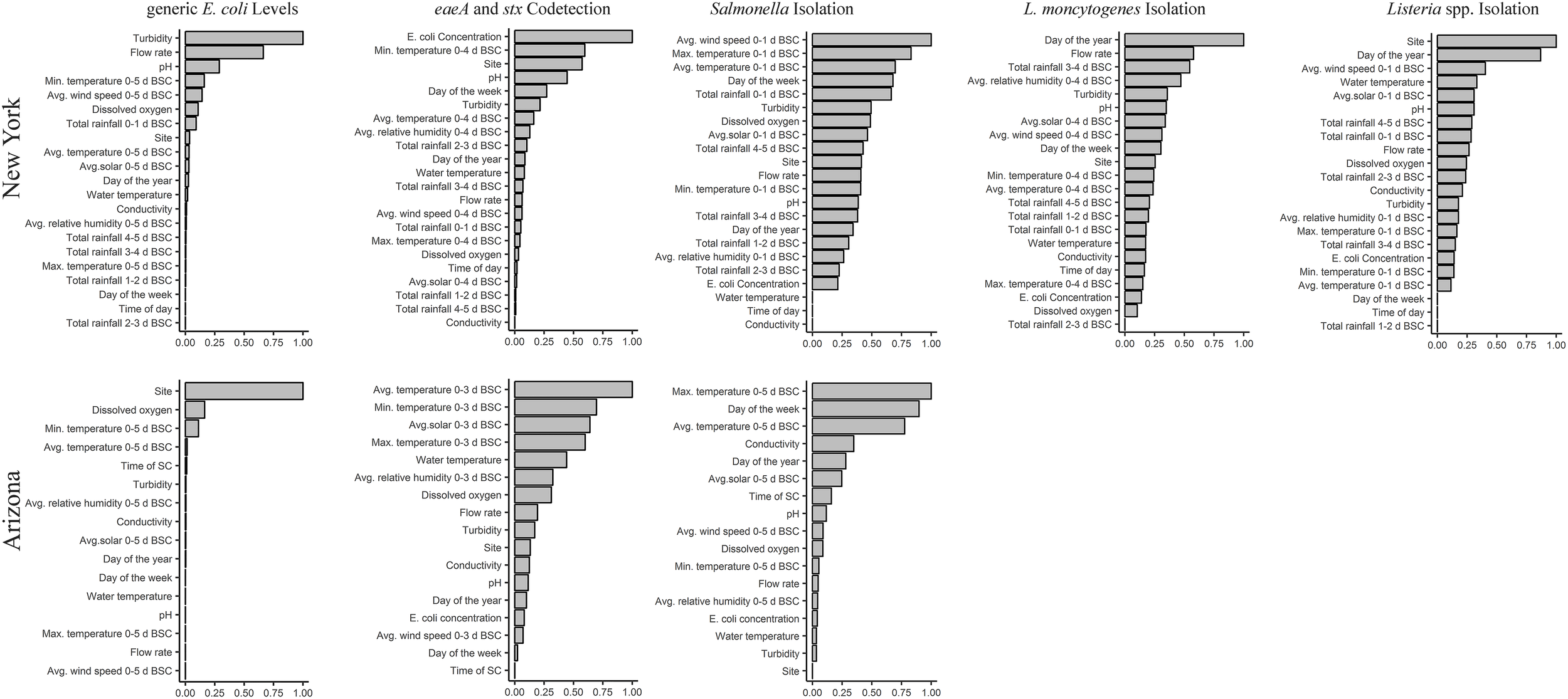
Results of random forest analyses that identified factors associated with E. coli levels, and the likelihood of codetecting eaeA and stx, and detecting Salmonella, L. monocytogenes, and Listeria spp. (including L. monocytogenes) in GS. The y-axis shows the factors ranked from most to least important. The x-axis shows NVI; a higher NVI (relative to all factors in the plot) equates to a stronger association between outcome and factor. NVI ≤ 0 indicates no association. Five, overlapping time frames (0–1, 0–2, 0–3, 0–4, or 0–5 days BSC) were used to calculate the values of the weather factors with the exception of rainfall; rainfall was calculated on a daily basis (0–1, 1–2, 2–3, 3–4, 4–5 days BSC). Separate forests were then developed for each outcome (e.g., E. coli levels in AZ, likelihood of Salmonella isolation in NY) and time frame in each state. The results for the forest with the highest Kappa score for each outcome are reported here. Thus, the time frame for the forest reported here differs for each combination of outcome and state. BSC, before sample collection.
L. monocytogenes in AZ and NY
Listeria monocytogenes was isolated from 4% (3/76) of AZ GS and 15% (27/181) of NY GS (Table 1). While L. monocytogenes was isolated from 0 of the 34 AZ MS, L. monocytogenes was isolated from 7% (6/86; Table 2) of NY MS. In total, L. monocytogenes was isolated from samples collected on 29 of the 117 sampling days where paired MS-GS were collected (Table 3). L. monocytogenes was detected by MS only on 5 sampling days (all paired GS were L. monocytogenes-negative) and by one or more paired GS but not by the MS on 23 sampling days (Table 3). According to generalized linear mixed modeling, the odds of isolating L. monocytogenes from MS was significantly lower than the odds of isolating L. monocytogenes from a paired GS [Odds Ratio (OR = 0.39); 95% Confidence Interval (CI) = 0.16, 0.97].
Random forest analysis could not be performed to identify factors associated with L. monocytogenes isolation in AZ due to the low L. monocytogenes prevalence in AZ. For random forests where L. monocytogenes isolation from NY GS or NY MS was the outcome, the forest with the highest Kappa score was based on weather 0–4 days BSC (κ = 0.06; Accuracy = 0.76) and 0-1 day BSC (κ = 0.37; Accuracy = 0.90), respectively (Supplementary Table S4). Random forest analysis identified flow rate as a top-ranked factor associated with L. monocytogenes isolation from GS and MS in NY (Figure 1 and Supplementary Figure S8). While the likelihood of L. monocytogenes isolation from GS decreased as flow increased from 0.0 to 1.0 m/s, the likelihood of L. monocytogenes isolation from MS increased as flow increased from 0.0 to 1.0 m/s (Supplementary Figure S9). The other top-ranked factors associated with L. monocytogenes isolation from GS were year-day, rainfall 3–4 days BSC, and avg. relative humidity 0–4 days BSC (Figure 1). Flow rate and year-day were among the top-ranked factors regardless of the time period BSC considered (Supplementary Table S7). The likelihood of L. monocytogenes isolation from NY GS decreased from May to July and increased from July to September (Supplementary Figure S8). Additionally, the likelihood of L. monocytogenes isolation from NY GS (i) increased as rainfall 3–4 days BSC increased from 0.0 to 2.0 cm, and (ii) decreased as avg. relative humidity 0–4 days BSC increased from 60% to 100% (Supplementary Figure S9). For NY MS the other top-ranked factors associated with L. monocytogenes isolation were pH, and min. and max. air temperature 0–1 days BSC (Supplementary Figures S8, S9).
Listeria spp. in AZ and NY
Listeria spp. (including L. monocytogenes) was isolated from 4% (3/76) of AZ GS and from 47% (85/181) of NY GS (Table 1). Listeria spp. was also isolated from 0 of the 34 AZ MS and 27% (23/86; Table 2) of NY MS. Listeria spp. was detected by MS only on 7 sampling days, and by one or more paired GS but not by the MS on 38 sampling days (Table 3). According to generalized linear mixed modeling, the odds of isolating Listeria spp. from MS was significantly lower than the odds of isolating Listeria spp. from a paired GS (OR = 0.24; 95% CI = 0.12, 0.48).
Random forest analysis could not be performed to identify factors associated with Listeria spp. isolation in AZ due to the low prevalence of Listeria spp. in AZ. For random forests where Listeria spp. isolation from NY GS or MS was the outcome, the forest with the highest Kappa score was based on weather 0–1 days BSC (κ = 0.36; Accuracy = 0.69) and 0-5 days BSC (κ = 0.35; Accuracy = 0.75), respectively (Supplementary Table S4). Random forest analysis identified site, year-day, avg. wind speed 0–1 days BSC and water temperature as the top-ranked factors associated with Listeria spp. isolation from NY GS (Figure 1); site and year-day were among the 4 top-ranked factors regardless of the time frame BSC considered (Supplementary Table S7). The likelihood of Listeria spp. isolation showed limited variation from May to July but increased from July to September (Supplementary Figure S9). Additionally, the likelihood of Listeria spp. isolation from GS (i) increased as the avg. wind speed 0–1 days BSC increased from 0 to 15 km/h, and (ii) decreased as water temperature increased from 10 to 23°C (Supplementary Figure S9). For NY MS the top-ranked factors associated with Listeria spp. isolation were rainfall 0–1 days BSC, min. and avg. air temperature 0–5 days BSC, and flow rate (Supplementary Figure S8).
Salmonella in AZ and NY
Salmonella was isolated from 34% (26/77) of GS and 64% (21/33) of MS collected in AZ, and from 44% (80/181) of GS and 57% (50/88) of MS collected in NY (Tables 1, 2). Salmonella was detected by the MS only on 30 sampling days, and by 1 or more paired GS but not by the MS on 21 sampling days (Table 3). The odds of isolating Salmonella from MS were 2.2 times greater than the odds of isolating Salmonella from a paired GS (OR = 2.2; 95% CI = 1.4, 3. 5).
For random forests where Salmonella isolation from AZ GS or MS was the outcome, the forest with the highest Kappa score was based on weather 0–5 days BSC (κ = 0.40; Accuracy = 0.72) and 0–3 days BSC (κ = 0.38; Accuracy = 0.84), respectively (Supplementary Table S5). According to random forest analysis, the two top-ranked factors associated with Salmonella isolation from AZ GS and MS were avg. and max. air temperature (Figure 1 and Supplementary Figure S8). The likelihood of Salmonella isolation from AZ GS (i) increased as avg. and max. air temperature increased from 13 to 30°C and from 20 to 41°C, respectively, and (ii) decreased as avg. and max. air temperature increased from 30 to 38°C and from 41 to 47°C, respectively (Supplementary Figure S10). The other top-ranked factors associated with Salmonella isolation from AZ GS were day of the week and conductivity; max. air temperature and day of the week were among the 4 top-ranked factors regardless of time period BSC considered (Supplementary Table S7). The likelihood of isolating Salmonella from AZ GS was highest for samples collected on Tuesday and Wednesday (Supplementary Figure S10). Additionally, the likelihood of isolating Salmonella from AZ GS increased as conductivity increased from 750 to 1,300 μS/cm (Supplementary Figure S10).
For random forests where Salmonella isolation from NY GS or MS was the outcome, the forest with the highest Kappa score for both GS BSC (κ = 0.18; Accuracy = 0.61) and MS BSC (κ = 0.11; Accuracy = 0.58) was based on weather 0–1 days BSC (Supplementary Table S5). According to random forest analysis, the top-ranked factors associated with Salmonella isolation from NY GS were avg. wind speed 0–1 days BSC, max and avg. air temperature 0–1 days BSC, and day of the week (Figure 1). The likelihood of Salmonella isolation from NY GS decreased as (i) avg. wind speed increased from 0 to 4 km/h, and (ii) avg. and max. air temperature increased from 10 to 19°C and from 15 to 26°C, respectively (Supplementary Figure S10). The likelihood of Salmonella isolation from NY GS increased as (i) avg. wind speed increased from 4 to 13 km/h, and (ii) avg. and max. air temperature increased from 19 to 26°C and from 26 to 33°C, respectively (Supplementary Figure S10). The likelihood of isolating Salmonella from NY GS was highest for samples collected on Sat. and lowest for samples collected on Wednesday (Supplementary Figure S10). For NY MS the top-ranked factors associated with Salmonella isolation were rainfall 3–4 and 4–5 days BSC, turbidity, and year-day (Supplementary Figure S10).
Codetection of eaeA and stx in AZ and NY
Forty-eight percent (44/83) of GS and 91% (30/33) of MS collected in AZ, and 69% (125/181) of GS and 88% (77/88) of MS collected in NY were PCR-screen positive for both eaeA and stx (Tables 1, 2). Both genes were detected by MS only on 23 sampling days, and by 1 or more paired GS but not by MS on 7 sampling days (Table 3). The odds of codetecting eaeA and stx in a MS was 6.5 times greater than the odds of codetecting eaeA and stx in a paired GS (OR = 6.5; 95% CI = 3.1, 13.6).
While random forest analysis could not be performed to identify factors associated with eaeA-stx codetection in AZ MS due to the limited number of eaeA and stx-negative MS, random forest analysis was performed to identify factors associated with eaeA-stx codetection in AZ GS. For random forests where eaeA-stx codetection in AZ GS was the outcome, the forest with the highest Kappa score was based on weather factors 0-3 days BSC (κ = 0.47; Accuracy = 0.74; Supplementary Table S6). The top-ranked factors associated with eaeA-stx codetection in AZ GS were avg. solar radiation 0–3 days BSC, and avg., max., and min., air temperature (Figure 1); avg. and max. air temperature were among the 4 top-ranked factors regardless of the time period BSC considered (Supplementary Table S7). The likelihood of eaeA-stx codetection in AZ increased as (i) avg. solar radiation 0–3 days BSC increased from 11 to 31 Ly, and (ii) avg., max., and min. air temperature 0–3 days BSC increased from 10 to 27°C, from 20 to 42°C, and from 1 to 18°C, respectively (Supplementary Figure S11). The likelihood of eaeA-stx codetection in AZ decreased as avg. air temperature and min. air temperature 0–3 days BSC increased from 27 to 36°C and from 18 to 28°C, respectively (Supplementary Figure S11).
For random forests with eaeA-stx codetection in NY GS and MS as the outcome, the forest with the highest Kappa score was based on weather factors 0-4 days BSC (κ = 0.52; Accuracy = 0.79) and 0–2 days BSC (κ = 0.24; Accuracy = 0.79), respectively (Supplementary Table S6). The top-ranked factors associated with eaeA-stx codetection in NY GS were pH, min. air temperature 0–4 days BSC, the MPN of E. coli/100 mL, and site (Figure 1); pH, E. coli levels, and site were among the 4 top-ranked factors regardless of the time period BSC considered (Supplementary Table S7). The likelihood of eaeA-stx codetection in the NY GS increased as (i) min. air temperature 0–4 days BSC increased from 5 to 15°C, and (ii) E. coli levels increased from 18 to 1,000 MPN/100-mL (Supplementary Figure S11). The likelihood of eaeA-stx codetection in the NY GS decreased as (i) pH increased from 7.4 to 8.8, and (ii) min. air temperature 0–4 days BSC increased from 15 to 18°C (Supplementary Figure S11). The top-ranked factors associated with codetecting eaeA and stx in NY MS were rainfall 3–4 days BSC, conductivity, flow rate, and avg. air temperature 0–2 days BSC (Supplementary Figure S8).
Effect of Two-Way Interactions on Microbial Water Quality
Due to the number of potential interactions that could have been investigated (e.g., 136 interactions per random forest), we focused on the impact of biologically plausible interactions on estimated E. coli levels, and likelihood of detecting pathogens in GS (see Supplementary Table S8 for a complete list). We focused on GS as opposed to MS because (i) approx. twice as many GS (N = 264) were collected as MS (N = 121), and (ii) GS are more commonly used to monitor surface water quality. Although the PDPs show evidence of threshold effects (stark differences in likelihood of detection above versus below a cut-off for a given factor), this may be a product of pseudoreplication, the sample size, the limited time span of the study, and/or the existence of true thresholds. Investigating these threshold effects is outside the scope of the current study, and the results of the PDPs need to be interpreted with caution.
We found evidence of interactions between multiple factors (Supplementary Figures S12–S19). For example, the likelihood of isolating Salmonella from AZ GS appeared to be higher when dissolved oxygen was <8.5 mg/L and air temperature was >20°C compared to when dissolved oxygen was >8.5 mg/L or air temperature was <20°C (Supplementary Figure S12). Similarly, estimated E. coli levels in AZ were higher when dissolved oxygen was <8.0 mg/L and air temperature was >28°C (Supplementary Figures S12, S13) compared to when dissolved oxygen was >8.0 mg/L or air temperature was <28°C. In AZ we also observed a synergistic interaction effect on likelihood of Salmonella isolation and likelihood of eaeA-stx codetection between dissolved oxygen and solar radiation, and between dissolved oxygen and water temperature (Supplementary Figure S12). We also found evidence of two-way interactions between turbidity and other factors (Supplementary Figures S14–S19). For instance, E. coli levels in NY were highest when rainfall 0–1 days BSC was >1 cm and turbidity was >10 NTU compared to when rainfall 0–1 days BSC was <1 cm or turbidity was <10 NTU (Supplementary Figure S14). In NY we also observed a synergistic interaction effect between turbidity and (i) rainfall 0–1 days BSC on the likelihood of isolating Salmonella, and (ii) flow rate on estimated E. coli levels (Supplementary Figure S15). Unlike the enteric targets, an antagonistic interaction effect on likelihood of L. monocytogenes isolation was observed for turbidity and rainfall 0–1 days BSC, and turbidity and flow rate (Supplementary Figure S15). Interactions between E. coli levels and other factors also appear to affect likelihood of pathogen detection (Supplementary Figures S16–S19). For instance, in AZ, likelihood of Salmonella isolation was lowest when E. coli levels were <200 MPN/100-mL and avg. air temperature was <20°C, compared to when E. coli levels were >200 MPN/100-mL or avg. air temperature was >20°C (Supplementary Figure S17). The likelihood of isolating Salmonella in NY GS appeared to be highest when E. coli levels were >1,350 MPN/100-mL and turbidity was >30 NTUs compared to when turbidity was <30 NTUs or E. coli levels were <1,350 MPN/100-mL (Supplementary Figure S18).
Relationship Between E. coli Levels and Pathogens in GS
The relationship between the log10 MPN of E. coli/100 mL and pathogen detection was characterized using generalized linear mixed models. Models could not be developed to characterize the relationship between Listeria isolation and E. coli levels in AZ due to the low prevalence of Listeria in AZ. According to these analyses, Salmonella isolation in AZ, and eaeA-stx codetection in AZ and NY were significantly associated with E. coli levels, but L. monocytogenes and Salmonella isolation in NY were not (Table 4). The odds of isolating Salmonella from AZ GS increased by a factor of 4 (95% CI = 1.5, 13.5) for each log10 increase in the MPN of E. coli/100-mL. The odds of codetecting eaeA and stx in AZ and NY GS increased by a factor of 50 (95% CI = 4.1, 621.9) and a factor of 18 (95% CI = 5.4, 62.9), respectively, for each log10 increase in the MPN of E. coli/100-mL.
TABLE 4
| Target | Fixed Effects | Variance of Random Effects (SDc) | |||
| Change in Oddsa | 95% CIb | P-value | Year-day | Site | |
| L. monocytogenes | |||||
| New York | 1.13 | 0.46, 2.77 | 0.786 | 0.5 (0.7) | 0.0 (0.0) |
| Listeria spp.d | |||||
| New York | 0.97 | 0.37, 2.52 | 0.943 | 2.3 (1.5) | 1.3 (1.2) |
| Salmonella | |||||
| Arizona | 4.43 | 1.46, 13.47 | 0.009 | 2.1 (1.4) | 0.0 (0.0) |
| New York | 1.53 | 0.71, 3.30 | 0.274 | 1.3 (1.1) | 0.2 (0.4) |
| eaeA and stx | |||||
| Arizona | 50.20 | 4.05, 621.88 | 0.002 | 12.1 (3.5) | 6.6 (2.6) |
| New York | 18.40 | 5.39, 62.86 | <0.001 | 1.1 (1.0) | 0.1 (0.3) |
Results of generalized linear mixed models that characterized the relationship between the log10 MPN of E. coli level/100-mL and pathogen detection in grab samples.
aChange in the odds of detecting the target organism for a log10 increase in the E. coli concentration. b95% Confidence Interval. cStandard Deviation. dIncludes L. monocytogenes. If only non-pathogenic Listeria spp. were included, the odds of detecting Listeria spp. excluding L. monocytogenes decreased (OR = 0.94; 95%CI = 0.40, 2.19; P = 0.876) for each log10 increase in the MPN of E. coli level/100-mL; the variance of year-day and site were 0.6 (0.8) and 0.9 (0.9), respectively.
We also assessed the predictive accuracy of the proposed FSMA standard [geometric mean < 126 CFUs/100-mL and STV < 410 CFUs/100-mL; (Food and Drug Administration, 2015)] to identify waterways with a high or low risk of pathogen presence at time of water use. Briefly, bootstrapping was used to simulate water sampling to create a microbial water quality profile (MWQP) composed of 20 samples (N = 10,000 MWQPs per waterway). The last GS selected for inclusion in each MWQP represented water quality at time of water use. The geometric mean and STV varied substantially among the simulated MWQPs for a given waterway (Figure 2). While approximately 50% of MWQPs in AZ and 27% of MWQPs in NY met the proposed FSMA standard (Figure 2 and Table 5), the percent of pathogen-positive MWQPs that met the standard ranged between 20% (eaeA-stx codetection in NY) and 72% (L. monocytogenes in AZ). In general, the efficacy of the proposed standard for identifying waterways contaminated by pathogens appears to be region and pathogen-specific. For instance, while the odds of E. coli levels exceeding the standard was 2.6 times greater for streams positive eaeA and stx compared to streams negative for both genes [DOR = 2.6], the odds of E. coli levels exceeding the standard were approx. equal for canals positive eaeA and stx, and for canals negative for both genes (DOR = 0.99). We also found that the odds of E. coli levels exceeding the standard was lower for L. monocytogenes-positive waterways compared to L. monocytogenes-negative waterways (DOR = 0.4 in AZ; DOR = 0.8 in NY).
FIGURE 2
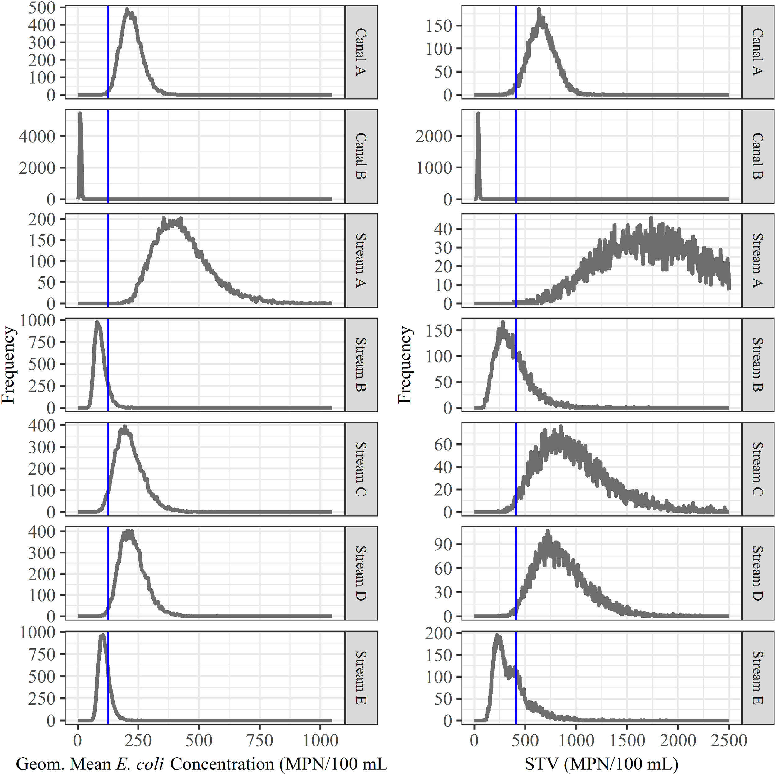
Bootstrapping was used to simulate water sampling to create microbial water quality profiles (MWQP) composed of 20 samples (N = 10,000 MWQPs per waterway). The graphs show the geometric mean and statistical threshold value (STV) for all MWQPs for each waterway. The blue line represents the proposed FSMA standard cut-offs (geometric mean < 126 CFU/100 mL and STV < 410 CFU/100 mL; Food and Drug Administration, 2015). Note that the y-axis varies between plots.
TABLE 5
| Target | Proportion of Pathogen Positive MWQPs that Met the Standarda | DORb | Sensitivity | Specificity |
| L. monocytogenes | ||||
| Arizona | 72% | 0.39 | 0.28 | 0.49 |
| New York | 32% | 0.75 | 0.68 | 0.26 |
| Listeria spp. | ||||
| Arizona | 72% | 0.39 | 0.28 | 0.49 |
| New York | 39% | 0.29 | 0.61 | 0.16 |
| Salmonella | ||||
| Arizona | 40% | 1.80 | 0.60 | 0.55 |
| New York | 27% | 1.03 | 0.74 | 0.27 |
| eaeA-stx | ||||
| Arizona | 51% | 0.99 | 0.49 | 0.50 |
| New York | 20% | 2.60 | 0.80 | 0.40 |
Ability of the proposed FSMA agricultural water standard (Food and Drug Administration, 2015) to predict L. monocytogenes, and Listeria spp., Salmonella isolation, and eaeA-stx codetection in agricultural water for a simulated dataset generated using a bootstrapping method.
aA simulated microbial water quality profile (MWQP) exceeded the proposed standard if the geometric mean was ≥126 CFUs/100 mL or the statistical threshold value was ≥410 CFUs/100 mL. In total, 50% of AZ subsets and 27% of NY subsets met the standard (regardless of pathogen status). bDiagnostic odds ratio = (Odds of E. coli levels exceeding the proposed thresholds in waterways contaminated by the target pathogen)/(Odds of E. coli levels exceeding the proposed thresholds in waterways not contaminated by the target pathogen). DOR < 1 indicates that not meeting the proposed standard is associated with a reduced risk of pathogen detection, a DOR ∼ 1 indicates that exceeding the proposed standard does not relate to pathogen contamination status, and a DOR > 1 indicates that exceeding the standard is associated with pathogen presence.
Discussion
This study was conducted to (i) characterize the relationship between E. coli levels and pathogen presence in agricultural water, and (ii) identify environmental factors associated with pathogen detection. This study is unique in its use of machine learning approaches (e.g., random forest analysis, partial dependence plots) to examine the impact of interactions between environmental factors on the likelihood of detecting foodborne pathogens or pathogen markers in agricultural water. This study also provided data on several understudied topics, including (i) the prevalence of food safety hazards in NY agricultural water, and (ii) the recovery of Listeria from surface water sources using Moore swabs (MS) compared to grab samples (GS). Overall, our study showed that sampling methods can affect reported pathogen prevalence and that environmental heterogeneity affects microbial water quality. Specifically, interactions between environmental factors (e.g., rainfall, turbidity) mediated the relationship between E. coli levels and likelihood of pathogen detection in the current study. As such, E. coli levels alone may not be a suitable indicator of the food safety risks associated with preharvest water use. Instead, alternative methods that utilize environmental and microbial data are needed to assess the food safety risks associated with preharvest water use. However, the findings reported here have to be viewed in the context of several limitations. For instance, the data reported here were collected from nine waterways over one growing season. Thus, additional studies are needed to determine if our findings are generalizable for the sampled waterways in future years, and to other waterways in AZ, NY, and other regions. Additionally, while the NY streams were randomly selected from all eligible streams, the AZ canals were enrolled based on convenience for the sampling team, which means that the AZ data may be affected by selection bias. For instance, a cattle feedlot was immediately upstream and next to Canal A, while feedlots were not present near Canals B and C. This could explain why Canal A had significantly higher E. coli levels than Canals B and C. Despite this limitation, our study highlights the variability in microbial water quality in AZ and is illustrative of the problems associated with using a single microbial indicator to identify when food safety hazards may be present in agricultural water. Despite the aforementioned limitations, our findings suggest that management of agricultural water-associated microbial food safety risks is not amenable to one-size-fits-all approaches due to the heterogeneous nature of freshwater environments. Instead, approaches that account for temporal variation in environmental conditions are needed.
Reported Pathogen Prevalence Differed When Different Sampling Methods Were Used
One objective of this study was to compare the ability of 24-h MS and 10-L GS to detect foodborne pathogens in surface water. Conceptually, a GS acts as a snapshot and provides data on water quality at a specific time, while MS capture bacteria that flow through the waterway over a given time period. We therefore hypothesized that MS would be better than GS at detecting pathogens. As predicted, the likelihood of Salmonella isolation, and eaeA-stx codetection was significantly greater for MS compared to GS. Past studies that compared the ability of MS and GS to detect pathogens in surface water reported similar results (Hoganson and Elliott, 1972; Colburn et al., 1990; Benjamin et al., 2013). For example, a California study that used MS and 100-mL GS found that the proportion of E. coli O157:H7-positive MS (13.8%; 12/87) was significantly greater than the proportion of O157:H7-positive GS (1.8%; 10/558; Benjamin et al., 2013). Unlike Salmonella isolation and eaeA-stx codetection, the likelihood of Listeria isolation was significantly lower for MS compared to GS in our study. One explanation for the lower than expected rate of Listeria detection by MS is that competitive microflora in the MS inhibited Listeria recovery. In fact, we observed more competitive microflora and fewer Listeria-like colonies when plating MS enrichments compared to paired GS enrichments. Past studies (Buzoleva and Terekhova, 2002; Francis and O’Beirne, 2002; Hansen et al., 2006; Habimana et al., 2011; McLaughlin et al., 2011; Locatelli et al., 2013), which found that the presence of other microflora inhibited Listeria survival support this hypothesis. Salmonella recovery may not have been affected by competitive microflora because samples used for Salmonella isolation underwent multiple selective enrichment steps while samples used for Listeria isolation underwent one selective, enrichment step. Overall, our findings indicate that appropriate water sampling methods depend on the reason for sample collection. Specifically, the organism of concern (e.g., AZ leafy green growers concerned about pathogenic E. coli may decide to use MS as opposed to GS), time constraints (MS require 2 site visits but GS require 1 visit), outcome of interest (e.g., MS cannot be used to calculate concentrations since the volume of water that flows through a MS is unknown), and the potential loss of MS (e.g., to storms, human tampering) should be considered when selecting a sampling method.
It is important to note that the L. monocytogenes prevalence in the current study was substantially lower than the prevalence reported by past studies that used the same enrichment and isolation protocols as this study (Strawn et al., 2013a, b; Chapin et al., 2014; Weller et al., 2015a, b). For instance, we isolated L. monocytogenes from 6% (2/32) of GS collected from Stream C, while studies that sampled Stream C at approx. the same site in 2013 and 2014 isolated L. monocytogenes from 71% (15/21; unpublished) and 63% [33/52; (Weller et al., 2015a)] of 250-mL GS, respectively. The larger sample volume in the current study required a change in GS processing; instead of filtering through a 0.45 um filter like previous studies (Strawn et al., 2013a, b; Chapin et al., 2014; Weller et al., 2015a, b), GS were filtered using mMS. We speculate that the lower than expected Listeria prevalence in the current study is because the mMS-method has not been optimized for Listeria recovery. Indeed, while several studies examined Salmonella and E. coli recovery using mMS (Bisha et al., 2011, 2014; McEgan et al., 2013b; Sbodio et al., 2013; Zhu et al., 2019), no study, to our knowledge, has quantified Listeria recovery using mMS. Such a study is needed if the mMS approach is to be incorporated into industry and government water testing programs as previously suggested (Bisha et al., 2014).
Microbial Water Quality Varied Across Time and Space
Random forest analysis identified associations between temporal factors and (i) E. coli levels, and (ii) the likelihood of pathogen detection. For example, year-day (number of days since Jan. 1, 2017) was among the top-ranked factors associated with L. monocytogenes and Listeria spp. isolation from NY GS. The identification of an association between year-day and microbial water quality suggests that microbial water quality varied seasonally, which is consistent with previous studies’ findings (Carter et al., 1987; Horman et al., 2004; Wilkes et al., 2009; Gorski et al., 2011; Cooley et al., 2014; Falardeau et al., 2017). For example, Falardeau et al. (2017) reported that L. monocytogenes was more prevalent in winter than summer in agricultural watersheds in British Colombia, Canada. Similarly, Cooley et al. (2014) found that the likelihood of isolating L. monocytogenes from California surface water samples was significantly higher in winter and spring compared to summer and fall. Cooley et al. (2014) and Falardeau et al. (2017) attributed this to increased rainfall and lower temperatures in winter and spring compared to summer and fall; seasonal patterns in temperature observed in the current study support this hypothesis. However, year-day may also serve as a proxy for unmeasured seasonal factors, such as anthropogenic reductions in water flow (e.g., damming of irrigation ditches) (Falardeau et al., 2017). While we did not observe this type of activity, all of the sampled waterways are in agricultural areas and provide water to commercial farms. As such, upstream activity that varied over the course of the growing season may have contributed to the seasonal variation in microbial water quality discussed above.
Microbial water quality and likelihood of pathogen detection also varied between waterways in our study. Sample site, which is unique to each waterway, was among the top-ranked factors associated with E. coli levels in AZ, and with Listeria spp. and eaeA-stx detection in NY GS. Given the number of factors that differ between waterways and may affect water quality, this is not surprising. In fact, multiple studies have found associations between microbial water quality and upstream land use (Lyautey et al., 2007; Pandey et al., 2012; Verhougstraete et al., 2015; Bradshaw et al., 2016; Brendel and Soupir, 2017; Dila et al., 2018). For instance, Pandey et al. (2012) tracked water quality at 46 sites in an Iowa watershed and found that E. coli levels were positively associated with the amount of cropland around each site. Associations between microbial water quality, and proximity to upstream livestock operations (Bond and Partyka, 2004; Lyautey et al., 2010; Wilkes et al., 2011), the number of septic systems in a watershed (Verhougstraete et al., 2015), and livestock and human population density (Falardeau et al., 2017; Dila et al., 2018) have also been reported. Post hoc identification of factors that drive spatial variation in water quality is difficult and requires data that were not collected as part of the current study. Despite this limitation, our findings indicate that microbial water quality varies between waterways. As such, future studies should consider the impact of spatial factors, in addition to weather and physicochemical water quality, when investigating associations between environmental conditions and microbial water quality.
Weather and Physicochemical Water Quality Were Associated With E. coli Levels as Well as the Likelihood of Detecting Foodborne Pathogens in Surface Water
Although the top-ranked factors associated with E. coli levels in AZ were site, DO, and air temperature, the variable importance scores (VI) for site and dissolved oxygen were substantially larger than the VI scores for air temperature. Similarly, the VI scores for turbidity, flow rate and pH, the 3 top-ranked factors associated with E. coli levels in NY, were substantially greater than the score for min. air temperature, the 4th-ranked factor. This suggests that E. coli levels were more strongly associated with physicochemical water quality than weather in the current study. Multiple studies have identified associations between physicochemical water quality and E. coli levels (Christensen et al., 2000; Horman et al., 2004; Roslev et al., 2004; Ansa et al., 2011; Rao et al., 2015; Stocker et al., 2016). A study that examined water quality along three Ecuadorian rivers found a negative association between dissolved oxygen and E. coli levels (Rao et al., 2015). One explanation for this inverse relationship between dissolved oxygen and E. coli levels is that the ability of UV radiation to damage bacterial cells is positively associated with dissolved oxygen (Curtis et al., 1992; Davies-Colley et al., 1997; Ansa et al., 2011; Ouali et al., 2014). While this hypothesis is supported by the NY data generated as part of the current study (E. coli levels in NY were highest when both dissolved oxygen and solar radiation were low), it is not supported by the AZ data reported here (E. coli levels in AZ were highest when dissolved oxygen was low and solar radiation was high). This discrepancy may be due to the correlation between solar radiation and temperature in AZ, which confounds the true nature of the interaction between dissolved oxygen and solar radiation.
While some studies identified an association between rainfall and microbial water quality (Wilkes et al., 2011; Pandey et al., 2012; Won et al., 2013; Francy et al., 2013; Stocker et al., 2016), other studies did not (Benjamin et al., 2013; McEgan et al., 2013a; Won et al., 2013). Interestingly, a survey of Florida water sources, which did not find an association between Salmonella levels and rainfall, hypothesized that rainfall did not have a direct effect on microbial water quality, and instead interacted with other factors to affect microbial water quality (McEgan et al., 2013a); our findings support this hypothesis. For example, we found evidence that interactions between rainfall and turbidity were associated with E. coli levels, Salmonella detection, and eaeA-stx detection in NY. Rainfall and turbidity are both indicative of conditions (e.g., increased surface run-off, flooding) that facilitate pathogen movement from environmental sources into streams, which may explain the synergistic interaction observed here. Stream sediments can also act as an in-channel store of bacteria, and disturbance of these sediments during rain events can re-introduce bacteria into the water column and concomitantly elevate turbidity levels (Nagels et al., 2002; Muirhead et al., 2004; Jamieson et al., 2005). However, due to the correlation between environmental factors in our study, determining the exact nature of the interactions observed requires additional data not collected and is beyond the scope of the present study. Despite this limitation, our findings suggest temporal environmental heterogeneity affects microbial water quality and should be taken into account when designing strategies for mitigating food safety risks associated with preharvest surface water use.
Even though our study found that complex interactions between weather and water quality factors were associated with microbial water quality, our findings also suggest relationships between specific factors and microbial water quality are reproducible. These factors may, therefore, be useful as supplemental indicators of microbial water quality. For example, multiple studies (Christensen et al., 2000; Nagels et al., 2002; Horman et al., 2004; Francy et al., 2013; Rao et al., 2015; Havelaar et al., 2017; Topalcengiz et al., 2017), including the study reported here and the Ecuadorian study discussed above (Rao et al., 2015), found a positive association between E. coli levels and temperature, or between E. coli levels and turbidity. Francy et al. (2013) surveyed recreational water quality at 22 Ohio beaches along inland lakes and found that turbidity was one of the best predictors of E. coli levels. Like the study presented here, previous studies have also found associations between turbidity and pathogen presence in surface water (Wilkes et al., 2011; Francy et al., 2013; Partyka et al., 2018). For instance, Wilkes et al. (2011) developed models to predict the presence of foodborne pathogens in Ontario, Canada surface water, and found that turbidity was an informative predictor of E. coli O157:H7 and L. monocytogenes presence.
Although we identified a relationship between temperature and model outcomes in 14 of the 15 random forests reported here, this relationship is complex and, as such, temperature may not be a suitable supplemental indicator of microbial water quality. For instance, temperature was correlated with several other factors (e.g., year-day, solar radiation), which obfuscates our ability to interpret the relationship between temperature and likelihood of pathogen detection. Moreover, based on the findings of this and other studies, the strength and direction of the relationship between temperature and microbial water quality appear to be pathogen, region, and/or waterway-specific (Francy et al., 2013; Luo et al., 2015; Truchado et al., 2018). Indeed, Francy et al. (2013) found that the strength and direction of correlation between water temperature and E. coli levels differed between the 22 Ohio lakes studied. Overall, the findings from this and other studies suggest that turbidity but not temperature may be a useful supplemental indicator of microbial water quality (Stocker et al., 2016; Havelaar et al., 2017).
The Relationship Between E. coli Levels and Pathogen Detection in Surface Water Appears to Be Mediated by Environmental Conditions
In the current study, we found that the relationship between E. coli levels and pathogen detection was region- and pathogen-specific. These findings are not unexpected since the relationship between E. coli levels and pathogen presence in surface water varied widely between past studies (Harwood et al., 2005; Wilkes et al., 2009; Benjamin et al., 2013; Economou et al., 2013; McEgan et al., 2013a; Pachepsky et al., 2015). Similarly, McEgan et al. (2013a) found that the relationship between E. coli and Salmonella levels varied substantially between 18 Florida waterways, and hypothesized that environmental factors mediated the relationship between E. coli and Salmonella levels in their study (McEgan et al., 2013a). Their hypothesis is supported by the findings of Bradshaw et al. (2016), who used classification trees to predict when Georgia waterways were contaminated by enteric pathogens and found that E. coli was a useful predictor only when certain conditions were met. Specifically, E. coli levels were useful for identifying (i) Salmonella-positive samples when dissolved oxygen < 11.3 mg/L and pH < 6.65, and (ii) stx-positive samples when air temperature ≥ 13°C (Bradshaw et al., 2016). These findings suggest that the relationship between E. coli levels and likelihood of pathogen presence may be weather, region, and/or pathogen-dependent. As such, the use of E. coli alone may not be a suitable indicator of different food safety risks associated with preharvest surface water use; this conclusion is consistent with other recent studies (e.g., Havelaar et al., 2017; Truitt et al., 2018).
Due to the continued use of E. coli to monitor agricultural water for potential food safety hazards (Food and Drug Administration, 2015; California Leafy Greens Marketing Agreement, 2017), understanding the effect of environmental conditions on the relationship between E. coli levels and pathogen presence in surface water is critical. This study sought to address this knowledge gap and found that interactions between E. coli levels and multiple environmental factors, including dissolved oxygen and turbidity, affected the strength and/or direction of the relationship between E. coli levels and one or more pathogens. One of the basic tenets of ecology is that different organisms will respond differently to the same conditions. One would therefore expect pathogens to respond to environmental conditions in a different manner than E. coli (e.g., Salmonella populations may persist while E. coli populations may die-off under a given condition). Indeed, multiple studies have shown that E. coli and foodborne pathogens respond differently to solar radiation (McCambridge and McMeekin, 1981; Sinton et al., 2007; Jenkins et al., 2011), and temperature (Rhodes and Kator, 1988; Martinez et al., 2014). In fact, a review that compiled findings on E. coli and Salmonella survival in non-host environments concluded that Salmonella was able to survive under a wider variety of environmental conditions and persist for longer in aquatic environments than E. coli (Winfield and Groisman, 2003). The variation in the relationship between E. coli levels and pathogen presence observed here and in other studies (e.g., McEgan et al., 2013a), may also be a product of the fact that sources of generic E. coli and specific pathogens may differ. Recent studies have found evidence that E. coli, including pathogenic E. coli and Salmonella can exist as autochthonous or naturalized populations in non-host environments [e.g., water (Hendricks, 1967; Goto and Yan, 2011; McEgan et al., 2013a), algal mats (Byappanahalli et al., 2003; Whitman et al., 2003; Ksoll et al., 2007), soil (Ishii et al., 2010; Nautiyal et al., 2010; Goto and Yan, 2011; NandaKafle et al., 2018)]. Thus, the co-occurrence of E. coli and foodborne pathogens in surface water environments is not necessarily evidence of a recent fecal contamination event but may instead result from conditions that facilitate the growth and survival of both organisms (McEgan et al., 2013a). Thus, our conclusion that environmental conditions mediate the relationship between E. coli levels and the likelihood of pathogen contamination of surface water sources is logical when viewed in the context of the existing ecological literature. By mediating the relationship between E. coli levels and pathogen presence in surface water, environmental conditions complicate interpretation of E. coli-based water test results, further illustrating the problems with using a single parameter (i.e., E. coli levels) as the primary basis for making decisions on how to best mitigate food safety risks associated with preharvest surface water use for produce production.
The Proposed FSMA Standard Is Not Indicative of the Food Safety Risks Associated With Preharvest Surface Water Use
It is important to consider how water testing results are interpreted when examining the use of E. coli as an indicator of potential food safety hazards in preharvest surface water. For example, the proposed FSMA standard states that growers must collect 20 samples over a 2 to 4 year period to create a microbial water quality profile (MWQP; Food and Drug Administration, 2015). The geometric mean E. coli level and STV of the MWQP must be ≤126 CFUs/100 mL and ≤410 CFUs/100 mL, respectively (Food and Drug Administration, 2015). We found that the geometric mean and STV varied substantially among the simulated MWQPs for each waterway; for instance, the geometric mean of the simulated MWQPs for Stream E varied between 56 and 265 MPN/100-mL. This indicates that meeting the proposed FSMA standard is largely a function of when the water samples that comprise the MWQP were collected, and that meeting the standard may be a poor approximation of E. coli levels in surface water at the time of water use. Additionally, when we quantified the ability of the proposed standard to identify the pathogen status of the simulated MWQPs, we found that the predictive accuracy of the proposed standard was poor with regard to predicting (i) eaeA-stx codetection, or L. monocytogenes detection in AZ canal water, and (ii) Salmonella or L. monocytogenes detection in NY stream water (DOR was less than or approximately 1). One limitation of this simulated sampling is that our samples were collected over one growing season while the proposed standard uses samples collected over 2–4 years to create the MWQP. However, our conclusions are logical given the temporal variation in the microbial quality of surface water observed in this and other studies (Goyal et al., 1977; Hipsey et al., 2008; Payment and Locas, 2011; Pandey et al., 2012) as well as our finding that the relationship between E. coli levels and pathogen presence was mediated by environmental conditions. Our conclusion is also consistent with that of Havelaar et al. (2017) who also examined the predictive accuracy of the proposed FSMA water quality standard and found that MWQPs consisting of 20 samples were insufficient to capture variability in E. coli concentrations in Floridian agricultural water. Overall these findings suggest that E. coli alone may not be a reliable indicator of the food safety risks associated with preharvest surface water use. The fact that other studies (Harwood et al., 2005; Ishii and Sadowsky, 2008; Benjamin et al., 2013; McEgan et al., 2013a; Pachepsky et al., 2015; Havelaar et al., 2017; Topalcengiz et al., 2017; Truitt et al., 2018) conducted in other regions, in other years, and using different protocols reached the same conclusion as the study reported here, suggests that our conclusion is robust despite limitations associated with our study’s observational nature and time frame.
Conclusion
Using advanced machine learning approaches this study showed that microbial water quality is associated with temporal environmental heterogeneity. As such, the food safety risks associated with preharvest use of a given surface water source are not constant over time and instead depend on environmental conditions at the time of water use. Our findings also indicate that (i) the relationship between E. coli levels and pathogen presence in surface water is mediated by environmental conditions, and (ii) E. coli levels alone may not be a suitable indicator of the food safety risks associated with preharvest surface water use. Instead, alternative approaches [e.g., e.g., models that incorporate data on E. coli levels and environmental conditions, incorporation of turbidity as a supplementary indicator into E. coli-based water quality monitoring programs] are needed to improve growers’ ability to identify and address these food safety risks in real-time. Given the dynamic and complex nature of surface water systems these alternative approaches need to (i) account for temporal variation in weather, and in physicochemical and water quality, and (ii) provide insights on microbial water quality at the time of water use.
Statements
Data availability statement
The R code and output from the random forest analyses are available at https://github.com/wellerd2/PAWQ-2017. The raw data is available upon request with some restrictions (e.g., location of sampling sites cannot be released); data requests should be directed to MW (martin.wiedmann@cornell.edu) or DW (wellerd2@gmail.com).
Author contributions
DW and MW conceived the project. DW, MW, and CR designed the study and wrote the grant. DW, MW, CR, and NB coordinated the efforts between the NY and AZ teams. DW and NB oversaw the day-to-day aspects of the project. DW, NB, SR, and EG carried out the field and laboratory work. DW, EM, and RI developed the data analysis plan, which DW implemented. DW wrote the manuscript with input from all other authors.
Funding
This research was largely funded by a grant from the Center for Produce Safety under award number 2017CPS09. Manuscript preparation was supported by the National Institute of Environmental Health Sciences of the National Institutes of Health (NIH) under award number T32ES007271. The content is solely the responsibility of the authors and does not represent the official views of the NIH.
Acknowledgments
We are grateful to Maureen Gunderson, Alexandra Belias, and Deniz Akdemir for the technical assistance. We are also grateful to Aziza Taylor, Kyle Markwardt, Sriya Sunil, Ahmed Gaballa, and Xiaodong Guo for the help in the field and the laboratory.
Conflict of interest
The authors declare that the research was conducted in the absence of any commercial or financial relationships that could be construed as a potential conflict of interest.
Supplementary material
The Supplementary Material for this article can be found online at: https://www.frontiersin.org/articles/10.3389/fmicb.2020.00134/full#supplementary-material
Abbreviations
- BSC
before sample collection
- CFU
colony-forming units
- DOR
Diagnostic odds ratio
- FSMA
Food Safety Modernization Act
- GS
grab sample(s)
- mMS
modified Moore swab(s)
- MPN
most probable number
- MS
Moore swab(s)
- MWQP
microbial water quality profile(s)
- NVI
normalized variable importance
- PDPs
partial dependence plot(s)
- STV
statistical threshold value
- VI
variable importance.
References
1
AlexanderL. M. (2015). Figuring Out The Food Safety Modernization Act. Available at: http://www.growingproduce.com/farm-management/(accessed January 28, 2020).
2
AnsaE. D. O.LubberdingH. J.AmpofoJ. A.GijzenH. J. (2011). The role of algae in the removal of Escherichia coli in a tropical eutrophic lake.Ecol. Eng.37317–324. 10.1016/J.ECOLENG.2010.11.023
3
AntakiM.VellidisG.HarrisC.AminabadiP.LevyK.Jay-RussellM. T. (2016). Low Concentration of Salmonella enterica and generic Escherichia coli in farm ponds and irrigation distribution systems used for mixed produce production in southern Georgia.Foodborne Pathog. Dis.13551–558. 10.1089/fpd.2016.2117
4
BalochM. A. (2014). “Leafy greens: the case study and real-life lessons from a Shiga-toxin-producing Escherichia coli (STEC) O145 outbreak in romaine lettuce,” in Global Safety of Fresh Produce: A Handbook of Best Practice, Innovative Commercial Solutions and Case Studies (Cambridge, UK: Woodhead Publishing), 340–355. 10.1533/9781782420279.5.340
5
BarrettT. J.BlakeP. A.MorrisG. K.PuhrN. D.BradfordH. B.WellsJ. G.et al (1980). Use of Moore swabs for isolating Vibrio cholerae from sewage.J. Clin. Microbiol.11385–388. 10.1128/jcm.11.4.385-388.1980
6
BatesD.MaechlerM.BolkerB.WalkerS. (2014). lme4: linear mixed-effects models using Eigen and S4.arxiv.org [Preprint]. Available at: http://arxiv.org/abs/1406.5823(accessed January 28, 2020).
7
BenjaminL.AtwillE. R.Jay-RussellM.CooleyM.CarychaoD.GorskiL.et al (2013). Occurrence of generic Escherichia coli, E. coli O157 and Salmonella spp. in water and sediment from leafy green produce farms and streams on the central California coast.Int. J. Food Microbiol.16565–76. 10.1016/j.ijfoodmicro.2013.04.003
8
BishaB.AdkinsJ. A.JokerstJ. C.ChandlerJ. C.Pérez-MéndezA.ColemanS. M.et al (2014). Colorimetric paper-based detection of Escherichia coli, Salmonella spp., and Listeria monocytogenes from large volumes of agricultural water.J. Vis. Exp.9. 10.3791/51414
9
BishaB.Perez-MendezA.DanylukM. D.GoodridgeL. D. (2011). Evaluation of modified moore swabs and continuous flow centrifugation for concentration of Salmonella and Escherichia coli O157:H7 from large volumes of water.J. Food Prot.741934–1937. 10.4315/0362-028X.JFP-11-133
10
BondR. F.PartykaM. L. (2004). Final Report for Source Identification, Optimized Monitoring, and Local Outreach for Reducing Animal Agricultural Inputs of Pathogens into the Sacramento-San Joaquin Delta Estuary; (04-122-555-0). Available at: http://www.vetmed.ucdavis.edu/atwill/local-assets/pdfs/DeltaFinalReport_2.9.4_04-122-555-0.pdf(accessed January 24, 2018).
11
BoryanC.YangZ.MuellerR.CraigM. (2011). Monitoring US agriculture: the US department of agriculture, national agricultural statistics service, cropland data layer program.Geocartol. Int.26341–358. 10.1080/10106049.2011.562309
12
BoulesteixA.-L.JanitzaS.HapfelmeierA.Van SteenK.StroblC. (2015). Letter to the Editor: on the term “interaction” and related phrases in the literature on random forests.Brief. Bioinform.16338–345. 10.1093/bib/bbu012
13
BradshawJ. K.SnyderB. J.OladeindeA.SpidleD.BerrangM. E.MeinersmannR. J.et al (2016). Characterizing relationships among fecal indicator bacteria, microbial source tracking markers, and associated waterborne pathogen occurrence in stream water and sediments in a mixed land use watershed.Water Res.101498–509. 10.1016/J.WATRES.2016.05.014
14
BrendelC.SoupirM. L. (2017). Relating watershed characteristics to elevated stream Escherichia coli levels in agriculturally dominated landscapes: an iowa case study.Water9154–172. 10.3390/w9030154
15
BundrantB. N.HutchinsT.den BakkerH. C.FortesE.WiedmannM. (2011). Listeriosis outbreak in dairy cattle caused by an unusual Listeria monocytogenes serotype 4b strain.J. Vet. Diagn. Invest.23155–158. 10.1177/104063871102300130
16
BustaF. F.SuslowT. V.ParishM. E.BeuchatL. R.FarberJ. N.GarrettE. H.et al (2006). The use of indicators and surrogate microorganisms for the evaluation of pathogens in fresh and fresh-cut produce.Compr. Rev. Food Sci. Food Saf.2179–185. 10.1111/j.1541-4337.2003.tb00035.x
17
BuzolevaL. S.TerekhovaV. E. (2002). Survivorship of different strains of the bacteria Listeria monocytogenes and Yersinia pseudotuberculosis in sea and river water.Russ. J. Mar. Biol.28259–262. 10.1023/A:1020225227751
18
ByappanahalliM. N.ShivelyD. A.NeversM. B.SadowskyM. J.WhitmanR. L. (2003). Growth and survival of Escherichia coli and enterococci populations in the macro-alga cladophora (Chlorophyta).FEMS Microbiol. Ecol.46203–211. 10.1016/S0168-6496(03)00214-9
19
California Leafy Greens Marketing Agreement, (2017). Commodity Specific Food Safety Guidelines for the Production and Harvest of Lettuce and Leafy Greens.Sacramento, CA: California Leafy Greens Marketing Agreement.
20
CarterA. M.PachaR. E.ClarkG. W.WilliamsE. A. (1987). Seasonal occurrence of Campylobacter spp. in surface waters and their correlation with standard indicator bacteria.Appl. Envir. Microbiol.53523–526. 10.1128/aem.53.3.523-526.1987
21
CastilloA.MercadoI.LuciaL. M.Martínez-RuizY.Ponce de LeónJ.MuranoE. A.et al (2004). Salmonella contamination during production of cantaloupe: a binational study.J. Food Prot.67713–720. 10.4315/0362-028x-67.4.713
22
Centers for Disease Control and Prevention (U.S.) (2018). Oubtreak of E. coli infections linkect to Romaine lettuce.Atlanta, GA: Centers for Disease Control and Prevention.
23
ChapinT. K.NightingaleK. K.WoroboR. W.WiedmannM.StrawnL. K. (2014). Geographical and meteorological factors associated with isolation of Listeria species in New York State produce production and natural environments.J. Food Prot.771919–1928. 10.4315/0362-028X.JFP-14-132
24
ChristensenV.JianX.ZieglerA. (2000). Regression Analysis and Real-Time Water-Quality Monitoring to Estimate Constituent Concentrations, Loads, and Yields in the Little Arkansas River, South-Central Kansas,1995-99 Water-Resources Investigations Report 00-4126. Available at: https://pubs.usgs.gov/wri/2000/4126/report.pdf(accessed January 28, 2020).
25
ColburnK. G.KaysnerC. A.AbeytaC.WekellM. M. (1990). Listeria species in a California coast estuarine environment.Appl. Environ. Microbiol.562007–2011. 10.1128/aem.56.7.2007-2011.1990
26
CooleyM. B.QuiñonesB.OryangD.MandrellR. E.GorskiL. (2014). Prevalence of shiga toxin producing Escherichia coli, Salmonella enterica, and Listeria monocytogenes at public access watershed sites in a California Central Coast agricultural region.Front. Cell. Infect. Microbiol.4:30. 10.3389/fcimb.2014.00030
27
CurtisT. P.MaraD. D.SilvaS. A. (1992). Influence of pH, oxygen, and humic substances on ability of sunlight to damage fecal coliforms in waste stabilization pond water.Appl. Environ. Microbiol.581335–1343. 10.1128/aem.58.4.1335-1343.1992
28
Davies-ColleyR. J.DonnisonA. M.SpeedD. J. (1997). Sunlight wavelengths inactivating faecal indicator microorganisms in waste stabilisation ponds.Water Sci. Technol.35219–225. 10.2166/wst.1997.0737
29
Den BakkerH. C.BundrantB. N.FortesE. D.OrsiR. H.WiedmannM. (2010). A population genetics-based and phylogenetic approach to understanding the evolution of virulence in the genus Listeria.Appl. Environ. Microbiol.766085–6100. 10.1128/AEM.00447-10
30
DeryJ. L.RockC. M.GoldsteinR. R.OnumajuruC.BrassillN.ZozayaS.et al (2019). Understanding grower perceptions and attitudes on the use of nontraditional water sources, including reclaimed or recycled water, in the semi-arid Southwest United States.Environ. Res.170500–509. 10.1016/J.ENVRES.2018.12.039
31
DilaD. K.CorsiS. R.LenakerP. L.BaldwinA. K.BootsmaM. J.McLellanS. L. (2018). Patterns of host-associated fecal indicators driven by hydrology, precipitation, and land use attributes in great lakes watersheds.Environ. Sci. Technol.5211500–11509. 10.1021/acs.est.8b01945
32
EconomouV.GousiaP.KansouzidouA.SakkasH.KaranisP.PapadopoulouC. (2013). Prevalence, antimicrobial resistance and relation to indicator and pathogenic microorganisms of Salmonella enterica isolated from surface waters within an agricultural landscape.Int. J. Hyg. Environ. Health216435–444. 10.1016/j.ijheh.2012.07.004
33
EdbergS. C.RiceE. W.KarlinR. J.AllenM. J. (2000). Escherichia coli: the best biological drinking water indicator for public health protection.J. Appl. Microbiol.88106S–116S. 10.1111/j.1365-2672.2000.tb05338.x
34
EricksonM. C.WebbC. C.Diaz-PerezJ. C.PhatakS. C.SilvoyJ. J.DaveyL.et al (2010). Surface and internalized Escherichia coli O157:H7 on field-grown spinach and lettuce treated with spray-contaminated irrigation water.J. Food Prot.731023–1029. 10.4315/0362-028x-73.6.1023
35
ESRI (2014). ArcGIS Desktop: Release 10.2.2. Redlands, CA: ESRI.
36
FalardeauJ.JohnsonR. P.PagottoF.WangS. (2017). Occurrence, characterization, and potential predictors of verotoxigenic Escherichia coli, Listeria monocytogenes, and Salmonella in surface water used for produce irrigation in the Lower Mainland of British Columbia, Canada.PLoS One12:e0185437. 10.1371/journal.pone.0185437
37
Food and Drug Administration (2015). Standards for the Growing, Harvesting, Packing, and Holding of Produce for Human Consumption.White Oak: Food and Drug Administration.
38
Food and Drug Administration (U.S.) (2018). Environmental assessment of factors potentially contributing to the contamination of Romaine lettuce implicated in a multi-state outbreak of E. coli O157:H7. Food and Drug Administration: White Oak.
39
FrancisG. A.O’BeirneD. (2002). Effects of the indigenous microflora of minimally processed lettuce on the survival and growth of Listeria innocua.Int. J. Food Sci. Technol.33477–488. 10.1046/j.1365-2621.1998.00199.x
40
FrancyD. S.StelzerE. A.DurisJ. W.BradyA. M. G.HarrisonJ. H.JohnsonH. E.et al (2013). Predictive models for Escherichia coli concentrations at inland lake beaches and relationship of model variables to pathogen detection.Appl. Environ. Microbiol.791676–1688. 10.1128/AEM.02995-12
41
GirardinH.MorrisC. E.AlbagnacC.DreuxN.GlauxC.Nguyen-TheC. (2005). Behaviour of the pathogen surrogates Listeria innocua and Clostridium sporogenes during production of parsley in fields fertilized with contaminated amendments.FEMS Microbiol. Ecol.54287–295. 10.1016/j.femsec.2005.04.003
42
GoreJ. (2006). “Discharge measurements and streamflow analysis,” in Methods in Stream Ecology, edsHauerF.LambertiG., (Burlington, MA: Elsevier), 69–70.
43
GorskiL.ParkerC. T.LiangA.CooleyM. B.Jay-RussellM. T.GordusA. G.et al (2011). Prevalence, distribution, and diversity of Salmonella enterica in a major produce region of California.Appl. Environ. Microbiol.772734–2748. 10.1128/AEM.02321-10
44
GotoD. K.YanT. (2011). Genotypic diversity of Escherichia coli in the water and soil of tropical watersheds in Hawaii.Appl. Environ. Microbiol.773988–3997. 10.1128/AEM.02140-10
45
GoyalS. M.GerbaC. P.MelnickJ. L.BonsdorffC.-H.von TorvelaN.HeikinheimoA.et al (1977). Occurrence and distribution of bacterial indicators and pathogens in canal communities along the Texas coast.Appl. Environ. Microbiol.34139–149. 10.1128/aem.70.1.87-95.2004
46
GreenwellB. M. (2017). Pdp: an R package for constructing partial dependence plots.R. J.9421–436.
47
GuanT. Y.BlankG.IsmondA.Van AckerR. (2001). Fate of foodborne bacterial pathogens in pesticide products.J. Sci. Food Agric.81503–512. 10.1002/jsfa.835
48
HabimanaO.GuillierL.KulakauskasS.BriandetR. (2011). Spatial competition with Lactococcus lactis in mixed-species continuous-flow biofilms inhibits Listeria monocytogenes growth.Biofouling271065–1072. 10.1080/08927014.2011.626124
49
HanW.YangZ.DiL.MuellerR. (2012). CropScape: a web service based application for exploring and disseminating US conterminous geospatial cropland data products for decision support.Comput. Electron. Agric.84111–123. 10.1016/J.COMPAG.2012.03.005
50
HanW.YangZ.DiL.YagciA. L.HanS. (2014). Making cropland data layer data accessible and actionable in GIS education.J. Geog.113129–138. 10.1080/00221341.2013.838286
51
HansenC. H.VogelB. F.GramL. (2006). Prevalence and survival of Listeria monocytogenes in Danish aquatic and fish-processing environments.J. Food Prot.692113–2122. 10.4315/0362-028X-69.9.2113
52
HarwoodV. J.LevineA. D.ScottT. M.ChivukulaV.LukasikJ.FarrahS. R.et al (2005). Validity of the indicator organism paradigm for pathogen reduction in reclaimed water and public health protection.Appl. Environ. Microbiol.713163–3170. 10.1128/AEM.71.6.3163-3170.2005
53
HavelaarA. H.VazquezK. M.TopalcengizZ.Muñoz-CarpenaR.DanylukM. D. (2017). Evaluating the U.S. food safety modernization act produce safety rule standard for microbial quality of agricultural water for growing produce.J. Food Prot.10.4315/0362-028X.JFP-17-122[Epub ahead of print].
54
HendricksC. (1967). Multiplication and growth of selected enteric bacteria in clear mountain stream water.Water Res.1567–576. 10.1016/0043-1354(67)90039-5
55
HipseyM. R.AntenucciJ. P.BrookesJ. D. (2008). A generic, process-based model of microbial pollution in aquatic systems.Water Resour. Res.44:W07408. 10.1029/2007WR006395
56
HogansonD. A.ElliottS. C. (1972). Bacteriological quality of lake red rock and the des moines river between des moines, iowa, and Lake Red Rock.Proc. Iowa Acad. Sci. U.S.A.7850–56.
57
HolvoetK.SampersI.SeynnaeveM.UyttendaeleM. (2014). Relationships among hygiene indicators and enteric pathogens in irrigation water, soil and lettuce and the impact of climatic conditions on contamination in the lettuce primary production.Int. J. Food Microbiol.17121–31. 10.1016/j.ijfoodmicro.2013.11.009
58
HormanA.Rimhanen-FinneR.MaunulaL.von BonsdorffC.-H.TorvelaN.HeikinheimoA.et al (2004). Campylobacter spp., Giardia spp., Cryptosporidium spp., Noroviruses, and indicator organisms in surface water in southwestern Finland, 2000-2001.Appl. Environ. Microbiol.7087–95. 10.1128/AEM.70.1.87-95.2004
59
IbenyassineK.AitMhandR.KaramokoY.CohenN.EnnajiM. M. (2006). Use of repetitive DNA sequences to determine the persistence of enteropathogenic Escherichia coli in vegetables and in soil grown in fields treated with contaminated irrigation water.Lett. Appl. Microbiol.43528–533. 10.1111/j.1472-765X.2006.01997.x
60
IjabadeniyiO. A.DebushoL. K.VanderlindeM.BuysE. M. (2011). Irrigation water as a potential preharvest source of bacterial contamination of vegetables.J. Food Saf.31452–461. 10.1111/j.1745-4565.2011.00321.x
61
IshiiS.SadowskyM. J. (2008). Escherichia coli in the environment: implications for water quality and human health.Microbes Environ.23101–108. 10.1264/jsme2.23.101
62
IshiiS.YanT.VuH.HansenD. L.HicksR. E.SadowskyM. J. (2010). Factors controlling long-term survival and growth of naturalized Escherichia coli Populations in temperate field soils.Microbes Environ.258–14. 10.1264/jsme2.ME09172
63
JamiesonR. C.JoyD. M.LeeH.KostaschukR.GordonR. J. (2005). Resuspension of sediment-associated Escherichia coli in a natural stream.J. Environ. Qual.34581–589. 10.2134/jeq2005.0581
64
JenkinsM. B.FisherD. S.EndaleD. M.AdamsP. (2011). Comparative die-off of Escherichia coli 0157:H7 and fecal indicator bacteria in pond water.Environ. Sci. Technol.451853–1858. 10.1021/es1032019
65
KayedD. (2004). Microbial Quality of Irrigation Water Used in the Production of Fresh Produce in Arizona.Tucson: University of Arizona. Ph.D. Thesis.
66
KimJ. S.LeeG. G.ParkJ. S.JungY. H.KwakH. S.KimS. B.et al (2007). A novel multiplex PCR assay for rapid and simultaneous detection of five pathogenic bacteria: Escherichia coli O157:H7, Salmonella, Staphylococcus aureus, Listeria monocytogenes, and Vibrio parahaemolyticus.J. Food Prot.701656–1662. 10.4315/0362-028x-70.7.1656
67
KsollW. B.IshiiS.SadowskyM. J.HicksR. E. (2007). Presence and sources of fecal coliform bacteria in epilithic periphyton communities of Lake Superior.Appl. Environ. Microbiol.733771–3778. 10.1128/AEM.02654-06
68
KuhnM. (2018). caret: Classification, and Regression Training. Available at: https://cran.r-project.org/package=caret(accessed January 28, 2020).
69
LenthR. (2018). emmeans: Estimated Marginal Means, aka Least-Squares Means. Available at: https://cran.r-project.org/package=emmeans(accessed January 28, 2020).
70
LocatelliA.SporA.JolivetC.PiveteauP.HartmannA. (2013). Biotic and abiotic soil properties influence survival of Listeria monocytogenes in soil.PLoS One8:e75969. 10.1371/journal.pone.0075969
71
LuoZ.GuG.GinnA.GiurcanuM. C.AdamsP.VellidisG.et al (2015). Distribution and characterization of Salmonella enterica isolates from irrigation ponds in the Southeastern U.S.A.Appl. Environ. Microbiol.814376–4387. 10.1128/AEM.04086-14
72
LyauteyE.LapenD. R.WilkesG.McClearyK.PagottoF.TylerK.et al (2007). Distribution and characteristics of Listeria monocytogenes isolates from surface waters of the South Nation River watershed, Ontario, Canada.Appl. Environ. Microbiol.735401–5410. 10.1128/AEM.00354-07
73
LyauteyE.LuZ.LapenD. R.WilkesG.ScottA.BerkersT.et al (2010). Distribution and diversity of Escherichia coli populations in the South Nation River drainage basin, eastern ontario Canada.Appl. Environ. Microbiol.761486–1496. 10.1128/AEM.02288-09
74
MartinezG.PachepskyY.WhelanG.YakirevichA. M.GuberA.GishT. J. (2014). Rainfall-induced fecal indicator organisms transport from manured fields: model sensitivity analysis.Environ. Int.63121–129. 10.1016/j.envint.2013.11.003
75
McCambridgeJ.McMeekinT. A. (1981). Effect of solar radiation and predacious microorganisms on survival of fecal and other bacteria.Appl. Environ. Microbiol.411083–1087. 10.1128/aem.41.5.1083-1087.1981
76
McEganR.MootianG.GoodridgeL. D.SchaffnerD. W.DanylukM. D. (2013a). Predicting Salmonella populations from biological, chemical, and physical indicators in Florida surface waters.Appl. Environ. Microbiol.794094–4105. 10.1128/AEM.00777-13
77
McEganR.RodriguesC. A. P. A. P.SbodioA.SuslowT. V. V.GoodridgeL. D. D.DanylukM. D. D. (2013b). Detection of Salmonella spp. from large volumes of water by modified moore swabs and tangential flow filtration.Lett. Appl. Microbiol.5688–94. 10.1111/lam.12016
78
McLaughlinH. P.CaseyP. G.CotterJ.GahanC. G. M.HillC. (2011). Factors affecting survival of Listeria monocytogenes and Listeria innocua in soil samples.Arch. Microbiol.193775–785. 10.1007/s00203-011-0716-7
79
MicallefS. A.Rosenberg GoldsteinR. E.GeorgeA.KleinfelterL.BoyerM. S.McLaughlinC. R.et al (2012). Occurrence and antibiotic resistance of multiple Salmonella serotypes recovered from water, sediment and soil on mid-Atlantic tomato farms.Environ. Res.11431–39. 10.1016/j.envres.2012.02.005
80
ModyR. K.GreeneS.GaulL.SeverA.PichetteS.ZambranaI.et al (2011). National outbreak of Salmonella serotype Saintpaul infections: importance of Texas restaurant investigations in implicating Jalapeño peppers.PLoS One6:e16579. 10.1371/journal.pone.0016579
81
MuirheadR. W.Davies-ColleyR. J.DonnisonA. M.NagelsJ. W. (2004). Faecal bacteria yields in artificial flood events: quantifying in-stream stores.Water Res.381215–1224. 10.1016/J.WATRES.2003.12.010
82
NagelsJ. W.Davies-ColleyR. J.DonnisonA. M.MuirheadR. W. (2002). Faecal contamination over flood events in a pastoral agricultural stream in New Zealand.Water Sci. Technol.4545–52. 10.2166/wst.2002.0408
83
NandaKafleG.ChristieA. A.VilainS.BrözelV. S. (2018). Growth and extended survival of Escherichia coli O157:H7 in soil organic matter.Front. Microbiol.9:762. 10.3389/fmicb.2018.00762
84
NautiyalC. S.RehmanA.ChauhanP. S. (2010). Environmental Escherichia coli occur as natural plant growth-promoting soil bacterium.Arch. Microbiol.192185–193. 10.1007/s00203-010-0544-1
85
NightingaleK. K.WindhamK.WiedmannM. (2005). Evolution and molecular phylogeny of Listeria monocytogenes isolated from human and animal listeriosis cases and foods.J. Bacteriol.1875537–5551. 10.1128/JB.187.16.5537-5551.2005
86
OliveiraM.ViñasI.UsallJ.AngueraM.AbadiasM. (2012). Presence and survival of Escherichia coli O157:H7 on lettuce leaves and in soil treated with contaminated compost and irrigation water.Int. J. Food Microbiol.156133–140. 10.1016/j.ijfoodmicro.2012.03.014
87
OualiA.JupsinH.GhrabiA.VaselJ. L. (2014). Removal kinetic of Escherichia coli and enterococci in a laboratory pilot scale wastewater maturation pond.Water Sci Technol69755–759. 10.2166/wst.2013.774
88
PachepskyY.SheltonD.DornerS.WhelanG. (2015). Can E. coli or thermotolerant coliform concentrations predict pathogen presence or prevalence in irrigation waters?Crit. Rev. Microbiol.42384–393. 10.3109/1040841X.2014.954524
89
PandeyP. K.SoupirM. L.HaddadM.RothwellJ. J. (2012). Assessing the impacts of watershed indexes and precipitation on spatial in-stream E. coli concentrations.Ecol. Indic.23641–652. 10.1016/j.ecolind.2012.05.023
90
PartykaM. L.BondR. F.ChaseJ. A.AtwillE. R. (2018). Spatiotemporal variability in microbial quality of western us agricultural water supplies: a multistate study.J. Environ. Qual.47939–948. 10.2134/jeq2017.12.0501
91
PaymentP.LocasA. (2011). Pathogens in water: value and limits of correlation with microbial indicators.Ground Water494–11. 10.1111/j.1745-6584.2010.00710.x
92
RaoG.EisenbergJ.KleinbaumD.CevallosW.TruebaG.LevyK.et al (2015). Spatial variability of Escherichia coli in rivers of northern coastal ecuador.Water7818–832. 10.3390/w7020818
93
RhodesM. W.KatorH. (1988). Survival of Escherichia coli and Salmonella spp. in estuarine environments.Appl. Environ. Microbiol.542902–2907. 10.1128/aem.54.12.2902-2907.1988
94
RobertsA. J.WiedmannM. (2006). Allelic exchange and site-directed mutagenesis probe the contribution of ActA amino-acid variability to phosphorylation and virulence-associated phenotypes among Listeria monocytogenes strains.FEMS Microbiol. Lett.254300–307. 10.1021/tx0502589
95
RoslevP.BjergbaekL. A.HesselsoeM. (2004). Effect of oxygen on survival of faecal pollution indicators in drinking water.J. Appl. Microbiol.96938–945. 10.1111/j.1365-2672.2004.02209.x
96
SbodioA.MaedaS.Lopez-VelascoG.SuslowT. V. (2013). Modified Moore swab optimization and validation in capturing E. coli O157:H7 and Salmonella enterica in large volume field samples of irrigation water.Food Res. Int.51654–662. 10.1016/j.foodres.2013.01.011
97
SintonL.HallC.BraithwaiteR. (2007). Sunlight inactivation of Campylobacter jejuni and Salmonella enterica, compared with Escherichia coli, in seawater and river water.J. Water Health5357–365. 10.2166/wh.2007.031
98
StockerM. D.Rodriguez-ValentínJ. G.PachepskyY. A.SheltonD. R. (2016). Spatial and temporal variation of fecal indicator organisms in two creeks in Beltsville, Maryland.Water Qual. Res. J. Canada51167–179. 10.2166/wqrjc.2016.044
99
StrawnL. K.FortesE. D.BihnE.NightingaleK. K.GröhnY. T.WoroboR. W.et al (2013a). Landscape and meteorological factors affecting prevalence of three food-borne pathogens in fruit and vegetable farms.Appl. Environ. Microbiol.79588–600. 10.1128/AEM.02491-12
100
StrawnL. K.GröhnY. T.WarchockiS.WoroboR. W.BihnE.WiedmannM. (2013b). Risk factors associated with Salmonella and Listeria monocytogenes contamination of produce fields.Appl. Environ. Microbiol.797618–7627. 10.1128/AEM.02831-13
101
StroblC.BoulesteixA.-L.KneibT.AugustinT.ZeileisA. (2008). Conditional variable importance for random forests.BMC Bioinform.9:307. 10.1186/1471-2105-9-307
102
StroblC.BoulesteixA.-L.ZeileisA.HothornT. (2007a). Bias in random forest variable importance measures: illustrations, sources and a solution.BMC Bioinform.8:25. 10.1186/1471-2105-8-25
103
StroblC.BoulesteixA.-L.ZeileisA.HothornT. (2007b). variable importance measures: illustrations, sources and a solution.BMC Bioinform.8:2.
104
StroblC.HothornT.ZeileisA. (2009). Party on! a new, conditional variable-importance measure for random forests available in the party package.Contrib. Res. J.114–17. 10.1186/1471-2105-14-119
105
TopalcengizZ.StrawnL. K.DanylukM. D.DanylukM.WebsterL.GorskiL. (2017). Microbial quality of agricultural water in Central Florida.PLoS One12:e0174889. 10.1371/journal.pone.0174889
106
TruchadoP.HernandezN.GilM. I.IvanekR.AllendeA. (2018). Correlation between E. coli levels and the presence of foodborne pathogens in surface irrigation water: establishment of a sampling program.Water Res.128226–233. 10.1016/J.WATRES.2017.10.041
107
TruittL. N.VazquezK. M.PfunterR. C.RideoutS. L.HavelaarA. H.StrawnL. K. (2018). Microbial quality of agricultural water used in produce preharvest production on the eastern shore of Virginia.J. Food Prot.811661–1672. 10.4315/0362-028X.JFP-18-185
108
VerhougstraeteM. P.MartinS. L.KendallA. D.HyndmanD. W.RoseJ. B. (2015). Linking fecal bacteria in rivers to landscape, geochemical, and hydrologic factors and sources at the basin scale.Proc. Natl. Acad. Sci. U.S.A.11210419–10424. 10.1073/pnas.1415836112
109
WallG.ClementsD.FiskC.StoeckelD.WoodsK.BihnE. (2019). Meeting report: key outcomes from a collaborative summit on agricultural water standards for fresh produce.Compr. Rev. Food Sci. Food Saf.18723–737. 10.1111/1541-4337.12434
110
WeiT. (2013). Corrplot: Visualization of a Correlation Matrix. R Package Version 0.73. Available at: http://cran.r-project.org/package=corrplot(accessed January 28, 2020).
111
WellerD.WiedmannM.StrawnL. (2015a). Spatial and temporal factors associated with an increased prevalence of L. monocytogenes in spinach fields in New York State.Appl. Environ. Microbiol.816059–6069. 10.1128/AEM.01286-15
112
WellerD.WiedmannM.StrawnL. K. (2015b). Irrigation is significantly associated with an increased prevalence of Listeria monocytogenes in produce production environments in New York State.J. Food Prot.781132–1141. 10.4315/0362-028X.JFP-14-584
113
WellerD. L.BeliasA.GreenH.WiedmannM.RoofS. (2019). Landscape, water quality, and weather factors associated with an increased likelihood of foodborne pathogen contamination of New York streams used to source water for produce production.Front. Sustain. Food Syst.3:124. 10.3389/FSUFS.2019.00124
114
WhitmanR. L.ShivelyD. A.PawlikH.NeversM. B.ByappanahalliM. N. (2003). Occurrence of Escherichia coli and enterococci in Cladophora (Chlorophyta) in nearshore water and beach sand of Lake Michigan.Appl. Environ. Microbiol.694714–4719. 10.1128/AEM.69.8.4714-4719.2003
115
WilkesG.EdgeT.GannonV.JokinenC.LyauteyE.MedeirosD.et al (2009). Seasonal relationships among indicator bacteria, pathogenic bacteria, Cryptosporidium oocysts, Giardia cysts, and hydrological indices for surface waters within an agricultural landscape.Water Res.432209–2223. 10.1016/j.watres.2009.01.033
116
WilkesG.EdgeT. A.GannonV. P. J.JokinenC.LyauteyE.NeumannN. F.et al (2011). Associations among pathogenic bacteria, parasites, and environmental and land use factors in multiple mixed-use watersheds.Water Res.455807–5825. 10.1016/j.watres.2011.06.021
117
WinfieldM. D.GroismanE. (2003). Role of nonhost environments in the lifestyles of Salmonella and Escherichia coli.Appl. Environ. Microbiol.693687–3694. 10.1128/AEM.69.7.3687-3694.2003
118
WonG.KlineT. R.LeJeuneJ. T. (2013). Spatial-temporal variations of microbial water quality in surface reservoirs and canals used for irrigation.Agric. Water Manag.11673–78. 10.1016/j.agwat.2012.10.007
119
ZhuL.TorresM.BetancourtW. Q.SharmaM.MicallefS. A.GerbaC.et al (2019). Incidence of fecal indicator and pathogenic bacteria in reclaimed and return flow waters in Arizona, USA.Environ. Res.170122–127. 10.1016/J.ENVRES.2018.11.048
Summary
Keywords
agricultural water, produce safety, Listeria, Salmonella, irrigation, E. coli
Citation
Weller D, Brassill N, Rock C, Ivanek R, Mudrak E, Roof S, Ganda E and Wiedmann M (2020) Complex Interactions Between Weather, and Microbial and Physicochemical Water Quality Impact the Likelihood of Detecting Foodborne Pathogens in Agricultural Water. Front. Microbiol. 11:134. doi: 10.3389/fmicb.2020.00134
Received
21 August 2019
Accepted
21 January 2020
Published
06 February 2020
Volume
11 - 2020
Edited by
David Rodriguez-Lazaro, University of Burgos, Spain
Reviewed by
Beatrix Stessl, University of Veterinary Medicine Vienna, Austria; Lisa Gorski, Western Regional Research Center (USDA-ARS), United States
Updates
Copyright
© 2020 Weller, Brassill, Rock, Ivanek, Mudrak, Roof, Ganda and Wiedmann.
This is an open-access article distributed under the terms of the Creative Commons Attribution License (CC BY). The use, distribution or reproduction in other forums is permitted, provided the original author(s) and the copyright owner(s) are credited and that the original publication in this journal is cited, in accordance with accepted academic practice. No use, distribution or reproduction is permitted which does not comply with these terms.
*Correspondence: Martin Wiedmann, martin.wiedmann@cornell.edu; mw16@cornell.edu
†Present address: Daniel Weller, Department of Biostatistics, University of Rochester, Rochester, NY, United States; Erika Ganda, Department of Animal Science, Pennsylvania State University, State College, PA, United States
This article was submitted to Food Microbiology, a section of the journal Frontiers in Microbiology
Disclaimer
All claims expressed in this article are solely those of the authors and do not necessarily represent those of their affiliated organizations, or those of the publisher, the editors and the reviewers. Any product that may be evaluated in this article or claim that may be made by its manufacturer is not guaranteed or endorsed by the publisher.