A Mathematical Modeling Approach to Uncover Factors Influencing the Spread of Campylobacter in a Flock of Broiler-Breeder Chickens

Despite continued efforts to improve biosecurity protocols, Campylobacter continues to be detected in the majority of commercial chicken flocks across Europe. Using an extensive data set of Campylobacter prevalence within a chicken breeder flock for over a year, multiple Bayesian models are presented to explore the dynamics of the spread of Campylobacter in response to seasonal variation, species-specificity, bird health, and total colonization prevalence. These models indicated that birds within the flock varied greatly in their response to bacterial challenge, and that this phenomenon had a large impact on the overall prevalence of different species of Campylobacter. Campylobacter jejuni appeared more frequently in the summer, while Campylobacter coli persisted for a longer duration, amplified by the most susceptible birds in the flock. Our study suggests that strains of Campylobacter that appear most frequently likely possess no demographic advantage, but are instead amplified due to the health of the birds that ingest it.

Introduction

Poultry meat has been decisively implicated as a leading infection route for campylobacteriosis in humans (EFSA Panel on Biological Hazards, 2011). With an estimated 450,000 cases a year in the UK, ~10% of which result in hospitalization (Strachan and Forbes, 2010), Campylobacter presents an important public health challenge, and an estimated £50 million annual economic burden to the UK (Tam and O'Brien, 2016). An investigation by Public Health England indicated the extent to which Campylobacter spp. dominated the commercial poultry industry: seventy-three percent of supermarket chicken carcasses were found to contain Campylobacter and seven percent of the outer packaging was similarly contaminated (Jorgensen et al., 2015). Consequently, preventing the spread of the bacteria to humans by reducing the number of colonized broiler flocks, i.e., chickens grown specifically for meat, at slaughter is as an urgent endeavor (Wilson et al., 2008).

Current attempts at tackling outbreaks of Campylobacter have largely focused around on-farm biosecurity measures; however, little impact in reducing incidence has been demonstrated (Hermans et al., 2011). This is predominantly due to the aggressive rate of proliferation once Campylobacter has entered a flock, and further complicated by uncertainty in the exact route of primary colonization. Specifically designed prevention methods are also marred by high genetic diversity of Campylobacter spp. (Tresse et al., 2017).

Campylobacter has historically been considered to be a gastrointestinal commensal of chickens, but recent studies suggest that, at least in some circumstances, they are pathogenic (Humphrey et al., 2014; Wigley, 2015). We here refer to birds being “colonized” and Campylobacter spp. “shed” where they could be detected from samples. Once an initial bird has become colonized by Campylobacter, colonization of the rest of the flock occurs very rapidly, usually within the course of a week (Evans and Sayers, 2000; Shreeve et al., 2000; Stern et al., 2001). The bacteria are spread via the fecal-oral route. After becoming newly-colonized, the host broiler spends a brief period in a non-infectious incubation period, before excreting the bacteria in its fecal and caecal matter. Surrounding susceptible broilers are then exposed to this via coprophagy (Shanker et al., 1990).

Understanding of the spread of Campylobacter is hindered by incomplete understanding of the transmission dynamics of the bacteria at farm level. Multiple strains of Campylobacter can simultaneously inhabit broiler flocks (Höök et al., 2005), with some strains appearing to dominate the flock at different times (De Cesare et al., 2008; Kudirkienė et al., 2010). It has been suggested that these dynamical behaviors are driven by the appearance of demographically superior strains that outcompete other strains (Calderón-Gómez et al., 2009) within the gut. However, another study suggests that strains are lost or transmitted randomly, regardless of their genotypic differences (Grant et al., 2005). Indeed, recent mathematical modeling approaches have demonstrated that stochastic simulations can effectively capture the broad dynamical differences between strains of equal demographic ability (Rawson et al., 2019).

An area of more recent study is the role played by “super shedders,” birds who consistently shed high amounts of Campylobacter in their feces, in the transmission dynamics of Campylobacter within a flock. The impact of “super shedders” has been well-documented as a key factor in the rapid spread of Salmonella throughout chicken flocks (Gopinath et al., 2012; Menanteau et al., 2018), but the impact on the dynamics of Campylobacter spread within broiler flocks is not well-studied. These “super-shedders” have been found experimentally to have fewer circulating heterophilic cells, but this does not appear to be a genetically acquired trait, nor the result of differences in adaptive immunity (Barrow et al., 2004). The presence of such super shedders in broiler flocks has been observed in an experimental study measuring Campylobacter prevalence (Achen et al., 1998), and it is reasonable to assume that this could have implications for the transmission dynamics within a flock. Despite the lack of studies amongst chickens, variation in fecal shedding of Campylobacter has been detected in cattle (Rapp et al., 2012).

Some factors affecting transmission are well-reported, if incompletely understood. The effect of seasonal variation on both the carriage rate, and number of Campylobacter found in the caeca, of colonized chickens has been noted (Wallace et al., 1997), with an increase often observed in the spring or summer. The exact timing of these peaks, however, varies within and among countries (Kovats et al., 2005), and experimental work is not always able to detect such an effect (Humphery et al., 1993). Less well-investigated is the impact of different species of Campylobacter competing within a flock. C. jejuni, the most common species, has been found in ~90% of British chicken flocks, compared with C. coli appearing in 10% of flocks (Jorgensen et al., 2011). This ratio has been reported by other studies in broiler flocks (Bull et al., 2006), with species rarely both being simultaneously present. It is not understood whether this is due to established strains suppressing new strains from emerging, demographic differences, or the short-lifespan of commercial broiler flocks not providing enough time for multiple species to colonize a flock. Under laboratory conditions, C. coli has been shown to have lower growth rates, motility, and invasiveness than C. jejuni (Aroori et al., 2013), potentially explaining its rarer appearance in chicken flocks. There is also some suggestion that C. coli is more commonly isolated from older, free-range, birds (Colles et al., 2008).

This study explores the impact of multiple factors on the transmission of multiple sequence types (STs) of Campylobacter amongst individual birds within a flock across 51 weeks. A broiler breeder flock, i.e., the parents of broiler/meat birds, was studied rather than a broiler flock, since the production period of around a year, compared to a small number of weeks for broiler birds, allows much greater potential to study the interaction of different Campylobacter strains over time. When interpreting the results, however, it should be noted that broiler breeder flocks will differ from broiler flocks with respect to, for example, host genetics, age, feed, and flock density. The majority of the Campylobacter genotypes (STs), however, have been isolated from other chicken flocks, most typically housed commercial broiler flocks (Colles et al., 2015).

We use a robust data set from Colles et al. (2015), which is currently the best available for monitoring the Campylobacter strain dynamics amongst individual birds within a commercially reared flock across 51 weeks. Through a Bayesian modeling approach we show the range of receptiveness to colonization throughout the flock, and highlight the role that more-susceptible, “super-shedder,” birds play in driving disease. The impact of seasonal variation is also investigated, and specific attention is given to differences between species of Campylobacter, so as to understand how certain strains persist at higher levels throughout the flock. Seven exploratory models are presented, each investigating a specific research question, analyzing the transition probabilities at both a flock-wide, and individual level.

A Bayesian approach is considered for this study due to the methodology's innate strengths in analyzing incomplete data (Dorazio, 2016), and enabling efficient inference of missing data. Numerical computations were carried out using the Just Another Gibbs Sampler (JAGS) program (Plummer, 2007), a Markov chain Monte Carlo (MCMC) sampling program utilizing Gibbs sampling.

Data

The field data used for this study were originally presented in Colles et al. (2015). Within a flock of 500 broiler breeders, 200 birds were labeled with leg-rings and monitored for a total of 51 weeks. Each week, 75 unique birds were picked at random from the labeled 200, and a swab was taken of the cloacal opening. These swabs were then tested for the presence of Campylobacter through standard culture methods, and positive samples were then genotyped by multi-locus sequence typing (MLST) of seven house-keeping genes, enabling the sequence type (ST) and species of the Campylobacter isolate to be specified. Further experimental details can be found in the original publication (Colles et al., 2015).

As such we build a dataset providing information on real-time evolution of Campylobacter prevalence and diversity throughout the flock. This is shown below in Figure 1, with all positive samples classified by species of Campylobacter.

FIGURE 1

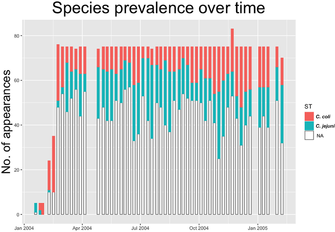
Figure 1. Histogram showing the count of positive and negative samples from a breeder flock for different species of Campylobacter. White “NA” counts represent samples that were negative for Campylobacter.

Within each species, multiple STs are recorded. In Figures 2, 3 below we plot the 5 weeks moving averages of total positive samples for each species. Beneath each point we plot a histogram showing how this average is split between the competing STs.

FIGURE 2

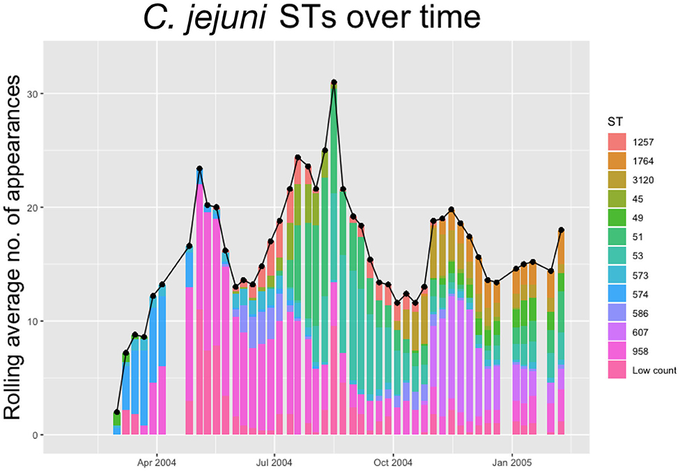
Figure 2. The 5-weeks rolling average number of positive samples for Campylobacter jejuni, with both the total number and separate ST averages. STs that appear <20 times throughout the entire experiment are amalgamated into a group “Low Count”.

FIGURE 3

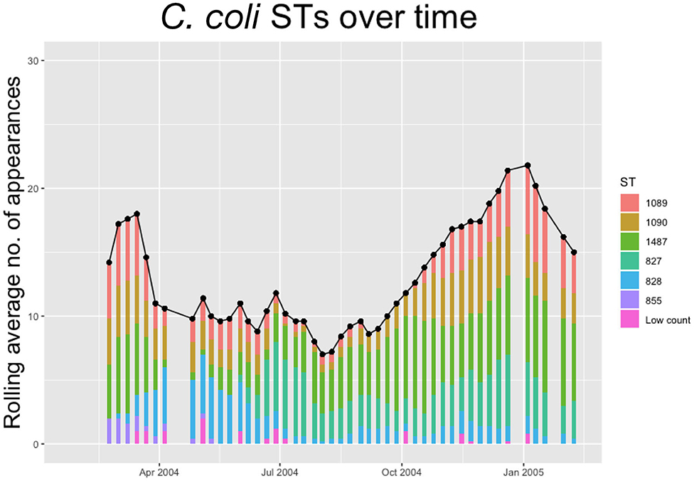
Figure 3. The 5-weeks rolling average number of positive samples for Campylobacter coli, with both the total number and separate ST averages. STs that appear <10 times throughout the entire experiment are amalgamated into a group “Low Count”.

We notice from Figures 2, 3 that there are more unique STs of C. jejuni than C. coli, despite both species existing at roughly equal levels. We also see that C. jejuni appears to peak in the summer, around the August period, coinciding with a dip in the population of C. coli STs. Within each species we can observe that different ST populations grow and shrink across the study period. For example, within Figure 2 we see that the summer peak is dominated by the prevalence of ST 51 and 53, however by November/December, this population shrinks, and instead ST 607 rapidly increases in population.

Figures 2, 3 effectively illustrate the key research questions tackled by this study. Namely, why do some STs seem to exist at higher quantities and persevere better than other STs which may die out? Do the dynamical behaviors of species and STs correlate to any particular trait? We investigate what mechanisms are dynamically driving these observed differences through querying the probability of chickens transitioning from different states of colonization using a series of Bayesian models presented below.

Model Development

In this section we discuss the general methodology behind all of our models. A general step-by-step process to model formulation is also presented in Box 1. Each model begins by classifying each of the datapoints into certain state labels. For example, at the simplest level each reading can be classified as either “State 1: Uncolonized” or “State 2: Colonized.” Other models may use more states to further distinguish colonizations by species or ST. After doing this, we are able to convey this classification data in the form of a matrix S[c, t] where c ∈ {1, 2, …, 200} is the index denoting which chicken is considered, and t ∈ {1, 2, …, 51} is the index denoting which week is considered. Therefore, each element of S will be a number conveying the state classification of that particular data point. For example, S[3, 7] = 1, would indicate that on week 7, chicken number 3 was classified as state 1; uncolonized. Because only 75 of the 200 chickens were tested at random each week, many of these matrix elements are undefined, and as such are marked as “NA.”

Box 1. Model construction process.

1. Decide state classifications.
Choose how data should be classified, and construct matrix S containing all state classifications for each data point.
2. Decide formulation of transition matrix.
Choose how model will define transition probabilities and dependencies.
3. Run Bayesian model.
Define prior probability distributions for model parameters. Program and run Bayesian model using JAGS, to acquire a posterior probability distribution for all model parameters defined in step 2.
4. Assess convergence.
Investigate model output to assure posterior distribution is well-constructed and has converged.
5. Present results.
Plot the transition probabilities, π_{i, j}, and interpret the results.

Once the matrix is defined, each model uses a Bayesian process to find the transition probabilities between these states. Formally we seek the matrix π, where π_{i, j} = P(S[m, n] = j|S[m, n − 1] = i), for every m ∈ {1, 2, …, 200} and n ∈ {2, 3, …, 51}. In short, π_{i, j} is the probability that a chicken moves from state i to state j across a week. The exact choice of how to formulate the expressions is where our models vary, as different formulations are able to investigate different relationships governing these transition probabilities. For example, at the simplest level, we could define

$\begin{array}{ll}\begin{array}{l}{\pi }_{1,1}={\alpha }_1\hfill \\ {\pi }_{1,2}=1-{\pi }_{1,1}\hfill \\ {\pi }_{2,1}={\alpha }_2\hfill \\ {\pi }_{2,2}=1-{\pi }_{2,1}\hfill \end{array}& (1)\end{array}$

where we seek to find the values α₁ ∈ [0, 1] and α₂ ∈ [0, 1] that best fit the data S. Note that we have bounded π_{i, j} between 0 and 1, as each value represents a probability. Likewise each row of π must sum to 1, as these probabilities cover all transition possibilities. In the example of Equation (1) above, when starting from state 1, one can transition to state 2 (π_1,2), or remain in state 1 (π_1,1), hence π_1,1 + π_1,2 = 1. Different models below will use more complex definitions for π to explore the impact of time, density dependence, and chicken health on transitions between different states.

A Bayesian statistical model provides a way to iteratively deduce parameters of interest in regards to given data. The process is derived from Bayes' theorem:

$\begin{array}{ll}P(\theta |D)=\frac{P(D|\theta )P(\theta )}{P(D)},& (2)\end{array}$

where θ is the parameter/s we wish to discover, and D is the data provided. In short, Equation (2) reads that when starting from an initial, prior, belief in what values θ may take (P(θ)), one may obtain an updated, posterior, probability distribution for these possible values given some provided data (P(θ|D)). A more thorough introduction to Bayesian modeling is provided in Appendix 1. In our case, the parameters we seek, θ, are the ones used in our definition of π, such as α₁ and α₂ in the example above. The data, D, we use is the matrix S.

Below we present a series of case studies presenting our different models and their results. All models were run using JAGS (Plummer, 2007) from within R using the run.jags package (Plummer et al., 2016). All code used for the following models is made available at https://osf.io/m5yua/.

Case Studies

Model 1: Time Dependence

Our first model investigates how time affects the transition probabilities between states. Following the process outlined in Box 1, we choose to initially classify our data as one of two states: “state 1: uncolonized” and “state 2: colonized.”

To assess how the transition probabilities vary through time we must ensure that we define our transition probabilities such that they depend on time. One way would be to adapt Equation (1) above such that π_1,1 was a function of α + βt. However, this would impose structure upon the transition probabilities, enforcing them to change linearly with time. Ideally a model formulation should allow as much freedom as possible to fit to the data. As such, we shall instead construct π as a three-dimensional array. In essence this means that each time period can be described by its own transition matrix. Formally we write this as,

$\begin{array}{ll}\begin{array}{l}{\pi }_{1,2,t}=\text{ilogit}({\alpha }_1+C_1[t]),\hfill \\ {\pi }_{1,1,t}=1-{\pi }_{1,2,t},\hfill \\ {\pi }_{2,1,t}=\text{ilogit}({\alpha }_2+C_2[t]),\hfill \\ {\pi }_{2,2,t}=1-{\pi }_{2,1,t},\hfill \end{array}& (3)\end{array}$

for t ∈ {1, 2, …, 51}. Here ilogit() is the inverse logit function defined by ilogit(x) = $\frac{e^x}{1+e^x}$. This function is bounded between 0 and 1, scaling the argument so that our probabilities, π_i,j,t remain correctly bounded. The underlying theory is that we assume there is some mean probability for π_i,j,t across all t. These mean probabilities are described by α₁ and α₂. We then assume that, for each t, there is some “correction term” away from the mean unique to each week. These correction terms are captured by C₁[t] and C₂[t] for each t.

Now that we have decided on our model formulation, we move to step 3 and run the model to find the posterior distributions for α₁, α₂, C₁, and C₂. First we define our prior probability distributions for each of the model parameters. This distribution represents our initial assumptions on what value our variables may take, and is often informed by expert opinion. Since we do not have any initial assumptions on what values our variables may take, we use wide non-informative priors. For α₁ and α₂ we choose a prior distribution of U(0, 25) for each, a uniform distribution between 0 and 25. For C₁ and C₂, we wish each element of these vectors to be a small perturbation away from the mean of α₁ or α₂. As such, we would ideally have these elements drawn from a normal distribution with mean 0, and some, yet to be determined, standard deviation. This represents a hierarchical model formulation (discussed further in Appendix 1), where we instead define priors on the two standard deviations for these two normal distributions associated with C₁ and C₂. Following the advice of Gelman (2006) for non-informative improper priors, we use a uniform distribution between 0 and 50 for the prior distribution of each of these standard deviation parameters. The model was then run using two chains, with a burn-in period of 5,000 iterations, and then a final sample of 25,000 iterations to build the posterior distributions.

Convergence was considered well-achieved via investigation of the trace plots of the chains, the effective sample size (ESS) and Monte Carlo Standard Error (MCSE) of the variables. The Gelman-Rubin statistic, or “shrink factor,” is the most commonly used metric for convergence, with a value close to 1 signifying effective convergence. Heuristically, any shrink factor below 1.1 is considered by Kruschke (2014) to signify sufficient convergence. The presented model run resulted in a multivariate potential scale reduction factor (mpsrf) of 1.0059.

The results for this model are presented below in Figure 4. The median values of the transition probabilities for (4A) π_1,1,t, (4B) π_1,2,t, (4C) π_2,1,t, (4D) π_2,2,t are plotted, and a linear regression is fit to these outputs using the lm function in R. Fitting a general additive model (GAM) to these median values revealed that there was no significant model fit for higher order models, hence only linear regression fits are displayed. The probability of transitioning from state 1 (plots 4A and 4B) was not significantly correlated against time (t-test, p = 0.135), however transitions from state 2 (plots 4C and 4D) against time were statistically significant (t-test, p < 0.01).

FIGURE 4

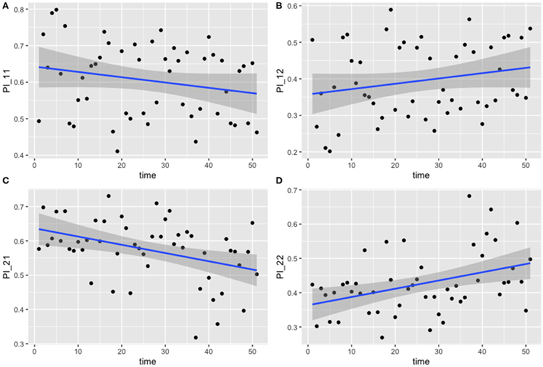
Figure 4. Transition probabilities between two states, “uncolonized” and “colonized.” Plots show (A) π_1,1,t, (B) π_1,2,t, (C) π_2,1,t, and (D) π_2,2,t against time. Each point is the calculated transition probability for that time point. Also plotted is a linear regression against these points in blue, with a shaded region depicting the 95% confidence interval of the regression. (C,D) Are significant (p < 0.01).

These findings suggest that, as time progresses, colonized chickens become more likely to remain colonized, and similarly become less likely to clear such a colonization. Figures 4C,D show that, at the start of the experiment, colonized chickens would be more likely to clear the colonization the following week, but by the end of the experiment this had reduced to a probability of roughly 50%.

Model 2: Species Dependence

For the next model we investigate transition differences between the two species present in the study: C. jejuni and C. coli. As such, this time we classify our data as belonging to one of three states; “state 1: uncolonized,” “state 2: colonized by C. jejuni,” and “state 3: colonized by C. coli.” Therefore our transition matrix will be of size 3 × 3. We define each row of the transition matrix by a 3-variable Dirichlet distribution (the multivariate generalization of the Beta distribution), ensuring each row sums to 1. As such, we infer the transition probabilities directly, using prior distributions of

$\begin{array}{l}({\pi }_{1,1},{\pi }_{1,2},{\pi }_{1,3})=\text{Dirichlet}(1,1,1),\\ ({\pi }_{2,1},{\pi }_{2,2},{\pi }_{2,3})=\text{Dirichlet}(1,1,1),\\ ({\pi }_{3,1},{\pi }_{3,2},{\pi }_{3,3})=\text{Dirichlet}(1,1,1).\end{array}$

The model was run with two chains and an initial burn-in period of 5,000 iterations. Posterior distributions were built from a sample of 10,000 iterations. Convergence was once again well-achieved with a mpsrf of 1.0035. The results are plotted below in Figure 5. Results show slight variations between species across the entire experiment. General transition probabilities from each state are very similar, however one can note that a chicken is more likely to be colonized by C. coli when transitioning from a state of already being colonized by C. coli. We also see that a chicken colonized by C. coli is less likely to transition to being uncolonized than a chicken colonized by C. jejuni.

FIGURE 5

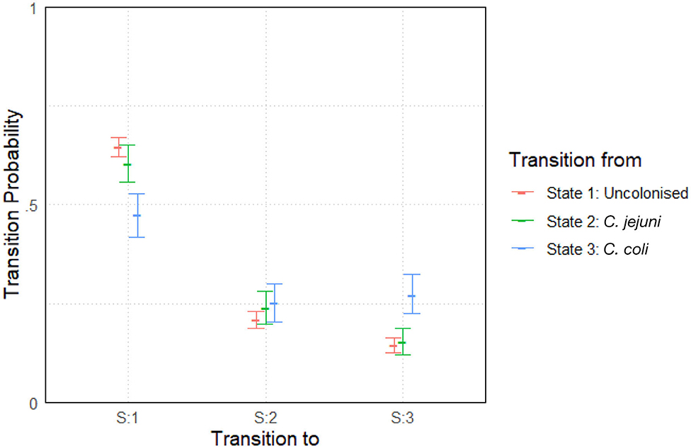
Figure 5. Transition probabilities between three states, “uncolonized,” “colonized by C. jejuni,” and “colonized by C. coli.” Plots show the median values of the posterior distributions and the 95% highest density intervals (HDIs).

Model 3: Time and Species Dependence

We now combine the previous two models together, to investigate how the transitions between species alter across time. We once again therefore classify our data into three categories, as per the previous model.

We will be constructing a three-dimensional array once again for our transition probabilities, with each time period being described by a separate 3 × 3 transition matrix. To ensure each row of these matrices sums to 1, we start by framing the transition probabilities as an unbounded array p, before scaling these into our final array π. p is defined as

$\begin{array}{ll}\begin{array}{ll}{p}_{1,1,t}=\text{exp}({\alpha }_1),\hfill & p_{1,2,t}=\text{exp}({\alpha }_2+C_1[t]),\hfill \\ p_{1,3,t}=\text{exp}({\alpha }_3+C_2[t]),\hfill & p_{2,1,t}=\text{exp}({\alpha }_4),\hfill \\ p_{2,2,t}=\text{exp}({\alpha }_5+C_3[t]),\hfill & p_{2,3,t}=\text{exp}({\alpha }_6+C_4[t]),\hfill \\ p_{3,1,t}=\text{exp}({\alpha }_7),\hfill & p_{3,2,t}=\text{exp}({\alpha }_8+C_5[t]),\hfill \\ p_{3,3,t}=\text{exp}({\alpha }_9+C_6[t]).\hfill \end{array}& (4)\end{array}$

The exponential function here assures that, like in our initial model, our α parameters will describe the average transition value across time, with the C parameters describing a small perturbation away from this mean. C values only need to be implemented on two probabilities in each row, as we will next scale these so that each row sums to 1, meaning that two free correction terms are sufficient to describe the distribution of the row. Our scaling is then performed like so,

$\begin{array}{l}{\pi }_{1,1,t}=\frac{p_{1,1,t}}{p_{1,1,t}+p_{1,2,t}+p_{1,3,t}},{\pi }_{1,2,t}=\frac{p_{1,2,t}}{p_{1,1,t}+p_{1,2,t}+p_{1,3,t}},\\ {\pi }_{1,3,t}=\frac{p_{1,3,t}}{p_{1,1,t}+p_{1,2,t}+p_{1,3,t}},{\pi }_{2,1,t}=\frac{p_{2,1,t}}{p_{2,1,t}+p_{2,2,t}+p_{2,3,t}},\\ {\pi }_{2,2,t}=\frac{p_{2,2,t}}{p_{2,1,t}+p_{2,2,t}+p_{2,3,t}},{\pi }_{2,3,t}=\frac{p_{2,3,t}}{p_{2,1,t}+p_{2,2,t}+p_{2,3,t}},\\ {\pi }_{3,1,t}=\frac{p_{3,1,t}}{p_{3,1,t}+p_{3,2,t}+p_{3,3,t}},{\pi }_{3,2,t}=\frac{p_{3,2,t}}{p_{3,1,t}+p_{3,2,t}+p_{3,3,t}},\\ {\pi }_{3,3,t}=\frac{p_{3,3,t}}{p_{3,1,t}+p_{3,2,t}+p_{3,3,t}}.& (5)\end{array}$

We choose priors of N(0, 1000) for all our α values (normal distributions with mean 0 and standard deviation 1,000). Like the first model, we shall construct a hierarchical dependency such that our C_i[t] are all drawn from a normal distribution for each t. Motivated by the correlation observed in the first model, we actually set these six C_i terms to all be drawn from a six-variable multivariate normal distribution, with mean (0, 0, 0, 0, 0, 0) and a covariance matrix as our parameter to be defined. JAGS requires the input of a precision matrix (the inverse of the covariance matrix) for its formulation of the multivariate normal distribution, so we set a prior distribution on the precision matrix of Wishart(I₆, 6), where I₆ is the 6 × 6 identity matrix.

The model was run with two chains for an initial burn-in period of 5,000 iterations, and then a posterior distribution was built from a sample of 250,000 iterations, thinned at a rate of 1 in 5, meaning only 1 in every 5 iterations was used for the posterior distribution so as to reduce autocorrelation. Results are plotted below in Figure 6.

FIGURE 6

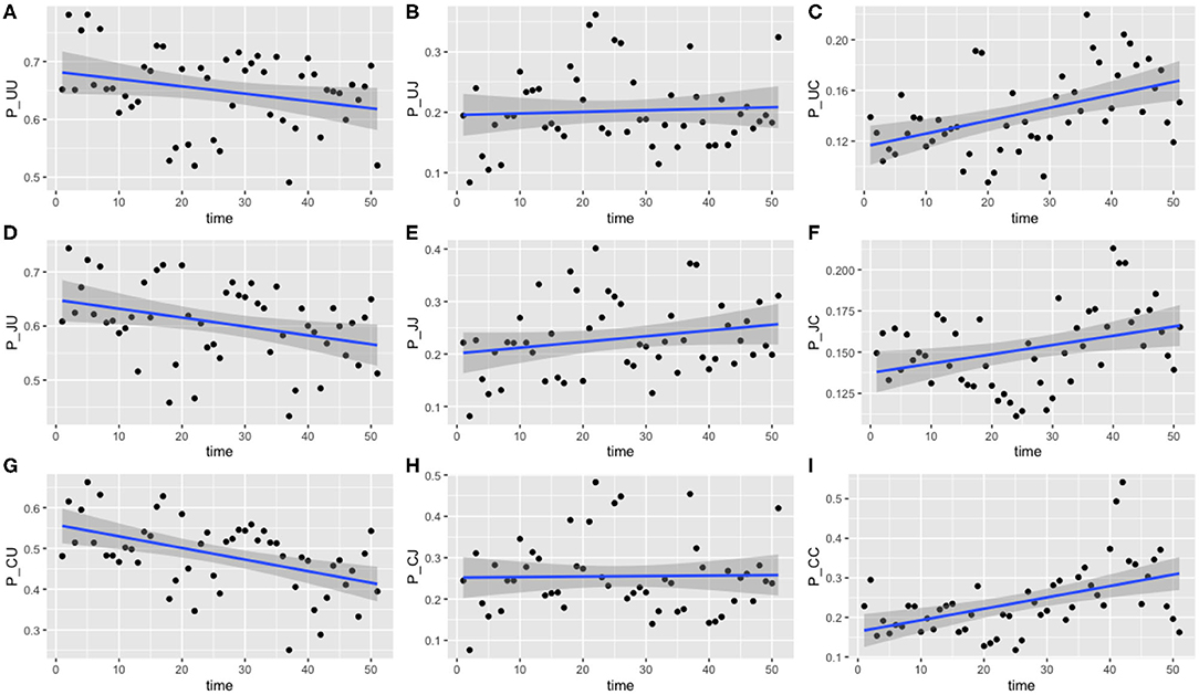
Figure 6. Transition probabilities between three states, “uncolonized,” “colonized by C. jejuni,” and “colonized by C. coli.” Plots show (A) π_1,1,t, (B) π_1,2,t, (C) π_1,3,t, (D) π_2,1,t, (E) π_2,2,t, (F) π_2,3,t, (G) π_3,1,t, (H) π_3,2,t, and (I) π_3,3,t against time. Each point is the calculated transition probability for that time point. Also plotted is a linear regression against these points in blue, with a shaded region depicting the 95% confidence interval of the regression. Five transition probabilities were found to be statistically significant for correlation against time: π_1,3,t, π_2,1,t, π_2,3,t, π_3,1,t, and π_3,3,t (t-tests, p < 0.0005, p < 0.05, p < 0.05, p < 0.0005, and p < 0.0005, respectively).

Of the nine transition probabilities presented, five were found to be statistically significant for correlation against time when a linear regression was applied: π_1,3,t, π_2,1,t, π_2,3,t, π_3,1,t, and π_3,3,t (t-tests, p < 0.0005, p < 0.05, p < 0.05, p < 0.0005, and p < 0.0005, respectively). We once again see that transitions to a state of uncolonization reduce over time, however, whereas model 1 reported overall transitions to a state of colonization increasing, model 3 shows that only transitions to colonization by C. coli increase over time. Given the spread of the data in Figure 6, we also tested for statistical significance against a quadratic regression. A quadratic fit would be a strong argument for the existence of seasonal variation, by capturing a difference in the middle of the time series as the time axis moves to summer, before returning to winter. Recall again that this time period plotted is in weeks from February 2004 to February 2005. Only one transition probability was found to be statistically significant however, the transition from colonization by C. jejuni to C. coli, π_2,3,t (t-test, p < 0.05). This quadratic regression is presented in Figure 7 below. This would correlate with the behavior observed in Figures 2, 3, whereby C. jejuni appears to be most prevalent in the summer, and C. coli most prevalent in the winter (similarly to model 1, fitting a general additive model (GAM) to these median values revealed that there was no significant model fit for higher order models, hence only linear regression fits, and the one quadratic regression fit, are displayed).

FIGURE 7

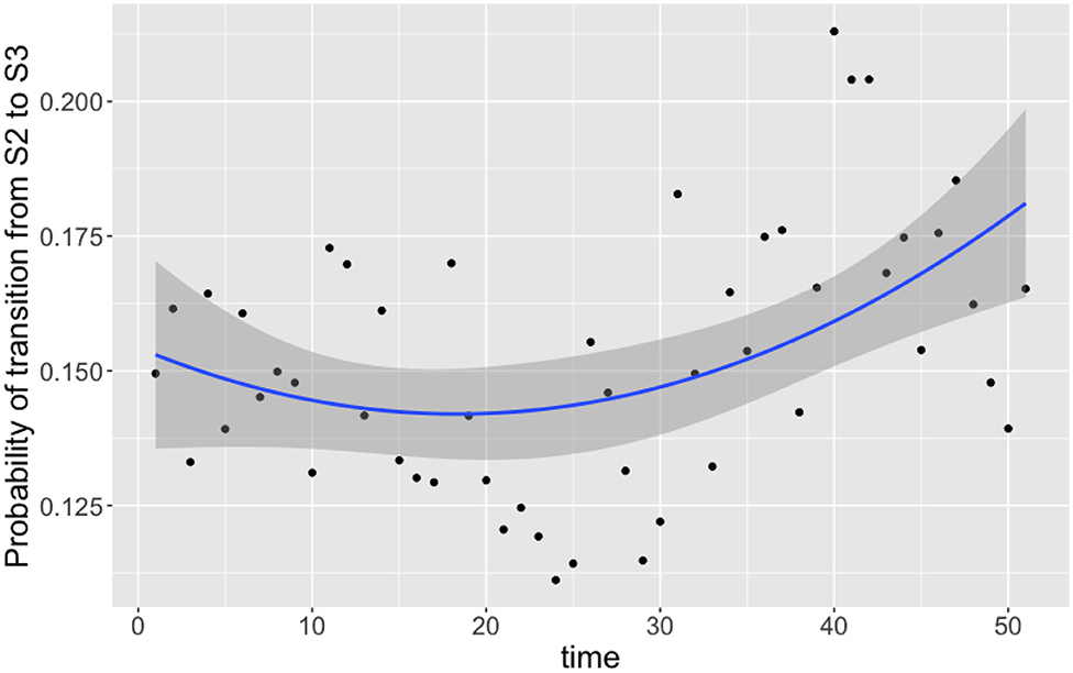
Figure 7. Transition probabilities between state 2 “colonized by C. jejuni” and state 3 “colonized by C. coli” against time. Each point is the calculated transition probability for that time point. Also plotted is a quadratic regression against these points in blue, with a shaded region depicting the 95% confidence interval. The transition probability was found to be statistically significant for correlation against time (t-test, p < 0.05).

Model 4: ST Perseverance

For this model, we extend model 2 to now capture species-specific ST perseverance within a chicken. To do this, we re-classify the data into five different states: “S1: uncolonized,” “S2: new C. jejuni ST,” “S3: same C. jejuni ST as previous week,” “S4: new C. coli ST,” and “S5: same C. coli ST as previous week.” To further clarify the meaning of state 2 and state 4, we mean a ST of either C. jejuni or C. coli that was not present in the previous week for the chicken in question. For example, if one chicken had the following colonization data for 10 days: {“Uncolonized,” “Colonized by C. coli ST 1089,” “Colonized by C. coli ST 1090,” “Colonized by C. coli ST 1090,” “NA,” “Colonized by C. coli ST 1090,” “Colonized by C. jejuni ST 958,” “Colonized by C. jejuni ST 958,” “Colonized by C. jejuni ST 1257,” “Uncolonized},” then this row of ten would be classified as { 1, 4, 4, 5, NA, 4, 2, 3, 2, 1 }. Because, by definition, one can only transition to state 3 from state 2 or state 3, we can fix π_1,3 = π_4,3 = π_5,3 = 0, and likewise for transitions to state 5: π_1,5 = π_2,5 = π_3,5 = 0. The non-zero transition probabilities can then be calculated by drawing each row from a 3 or 4 variable Dirichlet distribution. Formally we set a prior on each row of,

$\begin{array}{ll}\begin{array}{l}({\pi }_{1,1},{\pi }_{1,2},{\pi }_{1,4})~\text{Dirichlet}(1,1,1),\hfill \\ ({\pi }_{2,1},{\pi }_{2,2},{\pi }_{2,3},{\pi }_{2,4})~\text{Dirichlet}(1,1,1,1),\hfill \\ ({\pi }_{3,1},{\pi }_{3,2},{\pi }_{3,3},{\pi }_{3,4})~\text{Dirichlet}(1,1,1,1),\hfill \\ ({\pi }_{4,1},{\pi }_{4,2},{\pi }_{4,4},{\pi }_{4,5})~\text{Dirichlet}(1,1,1,1),\hfill \\ ({\pi }_{5,1},{\pi }_{5,2},{\pi }_{5,4},{\pi }_{5,5})~\text{Dirichlet}(1,1,1,1).\hfill \end{array}& (6)\end{array}$

The model was run with two chains for a burn-in period of 5,000 iterations before building posteriors from a final sample of 10,000 iterations. Chains were well-mixed and convergence well-achieved with an mpsrf of 1.0037. Results are plotted below in Figure 8.

FIGURE 8

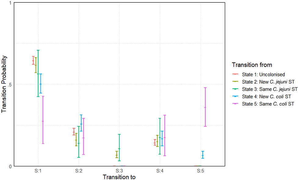
Figure 8. Transition probabilities between five states, “uncolonized,” “colonized by a new C. jejuni ST,” “colonized by the same C. jejuni ST as previously,” “colonized by a new C. coli ST,” and “colonized by the same C. coli ST as previously.” Plots show the median values of the posterior distributions and the 95% highest density intervals (HDIs).

The most notable difference is seen in the perseverance of C. coli STs compared to C. jejuni STs. Comparing columns 3 and 5 of Figure 8, we see that, a colonization by a new ST of either C. coli or C. jejuni has a roughly equal chance of persevering to the next week. However, once a ST has carried over for 1 week, C. coli colonizations are then considerably more likely to further persist for later weeks. In fact, a repeated instance of colonization by a C. coli ST (state 5) is more likely to continue in subsequent weeks than to transition to any other state (seen by comparing the pink lines in Figure 8). Comparing also columns 2 and 3 of Figure 8, we see that transitions to colonizations by new hboxtextitC. coli/C. jejuni STs are roughly comparable, meaning that the primary difference we observe between the two species is in perseverance as opposed to infectivity.

Model 5: Chicken Dependence

Whereas model 1 considered how transition probabilities vary across time, we now consider how transition probabilities vary across different chickens. We follow a very similar framework to model 1, beginning by classifying all data as one of two states: “S1: uncolonized” or “S2: colonized.” We then, like model 1, consider some average transition probability that each chicken is close to, and then consider some small “correction term” unique to each chicken, which may make them more or less likely to transition to a certain state. Formally, we write,

$\begin{array}{ll}\begin{array}{l}{\pi }_{1,2,t}=\text{ilogit}({\alpha }_1+C_1[c]),\hfill \\ {\pi }_{1,1,t}=1-{\pi }_{1,2,t},\hfill \\ {\pi }_{2,1,t}=\text{ilogit}({\alpha }_2+C_2[c]),\hfill \\ {\pi }_{2,2,t}=1-{\pi }_{2,1,t},\hfill \end{array}& (7)\end{array}$

for c ∈ {1, 2, …, 200}. We set a non-informative prior distribution for α₁ and α₂ of N(0, 1000). Our chicken correction terms, C₁[c] and C₂[c], are each drawn from a two-variable multivariate normal distribution for each c, with mean (0, 0) and covariance matrix to be calculated. Like described in model 3, we therefore set a prior distribution on the precision matrix for this multi-variate normal distribution of Wishart(I₂, 2), where I₂ is the 2 × 2 identity matrix.

The model was run with two chains for an initial burn-in period of 20,000 iterations, before posteriors were then constructed from a sample of 50,000 iterations. Convergence was well-achieved, with all chains well-mixed and all parameters sampled with a high ESS and MCSE < 0.01. The mpsrf was unable to be calculated due to the high number of stochastic nodes, however there were no signs to suggest invalid convergence.

Upon calculating our transition probabilities for each bird, we plot the values for π_1,2 against the value of π_2,1 for each bird and investigate the correlation. Figure 9 shows these results overlaid with a contour of the associated multivariate normal distribution, indicating the probability density of the transition probabilities for the flock.

FIGURE 9

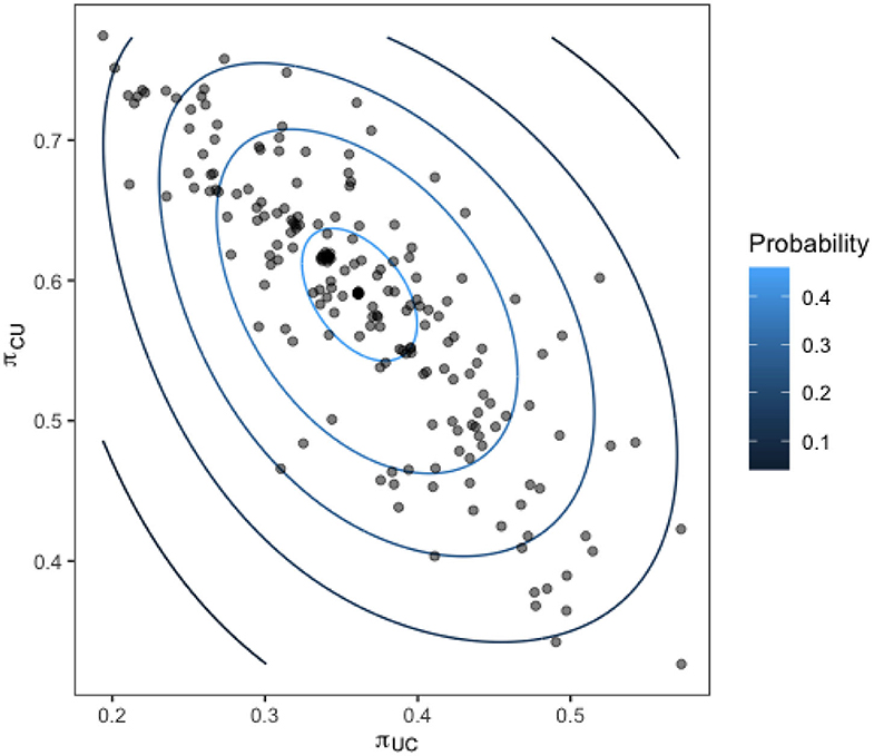
Figure 9. Transition probabilities for each bird in the flock from a state of being colonized to uncolonized (y-axis) against the transition probability from uncolonized to colonized (x-axis). Contours show the fit of a multivariate normal distribution to the output.

The strong linear relation observed reveals the presence of distinct sub-groups within the flock of birds who are colonized often, and those who are colonized very rarely.

Model 6: Chicken and Species Dependence

We now alter the previous model to consider the differences in transition between species of Campylobacter across all birds. As such, the data is instead classified into the three states: “state 1: uncolonized,” “state 2: colonized by C. jejuni,” and “state 3: colonized by C. coli.” This model is formulated the same way as in model 3 above. The transition probabilities follow the same structure as Equations (4) and (5), except that our correction terms C_i[c] are corrections for each chicken in the flock (c ∈ {1, 2, …, 200}) as opposed to each time step. As such we craft a 3 × 3 transition matrix for each chicken. A prior distribution of N(0, 1000) is used for each α_i parameter, and the six chicken correction terms, C_i[c] are drawn from a six-variate multivariate normal distribution for each c, with mean (0, 0, 0, 0, 0, 0) and a precision matrix as a parameter to find. The prior distribution for this precision matrix is Wishart(I₆, 6), where I₆ is the 6 × 6 identity matrix.

The model was run with two chains for an initial burn-in period of 10,000 iterations, before posterior distributions were constructed from a sample of 50,000 iterations, thinned at a rate of 1 in 25, meaning only one iteration was kept in every 25.

The idea of this model is to assess how bird variation affects the transition of each species of Campylobacter. The previous model revealed the existence of variation in bird resistance to colonization throughout the flock. Figure 10 below plots the result of multiple transition probabilities against one-another. Each point on the graphs represents the transition probabilities for a specific chicken. Plots 10A–C use π_1,1,c, the transition from uncolonized to uncolonized as the y-axis. This acts as a rough metric for “bird resilience to colonization,” as the more resistant birds are more likely to continue being uncolonized. As such plots 10A–C depict how transitions related to each species vary according to host bird susceptibility. Plot 10D uses π_3,3,c, the transition from C. coli to C. coli as the y-axis, to compare how the perseverance of C. coli affects the colonizing ability of C. jejuni. Linear regressions are fit to all plots in Figure 10, and all were found to be statistically significant (t-test, p < 0.0001).

FIGURE 10

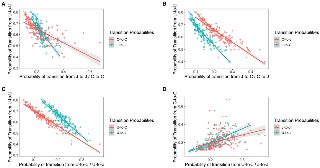
Figure 10. Transition probabilities for a three state system. In these plots, “U” refers to being uncolonized, “J” refers to colonization by C. jejuni and “C” refers to colonization by C. coli. Each of the points is the transition probability for a specific bird within the flock. Linear regression fits are plotted with a shaded region representing the 95% confidence intervals of the regression. All regressions were statistically significant (t-test p < 0.0001). (A) The transition probabilities of J-to-J and C-to-C against the transition probability of U-to-U. (B) The transition probabilities of C-to-J and J-to-C against the transition probability of U-to-U. (C) The transition probabilities of U-to-J and U-to-C against the transition probability of U-to-U. (D) The transition probabilities of J-to-J and U-to-J against the transition probability of C-to-C.

Interestingly, the gradients of all the shifting transition probabilities are different between species, confirming that, indeed, the transition probabilities of each species varies differently across chickens. We see that the probability of a species persisting, unsurprisingly increases as bird susceptibility increases, but curiously our linear regressions for each species overlap. This result indicates that, in the more resilient birds, C. coli is less likely to persevere than C. jejuni colonizations, however the inverse is seen in the more susceptible birds.

It is interesting to note that the gradient of the lines in each plot are distinctly different from one another, highlighting how each species responds differently to variations in host bird health.

Model 7: Chicken and Density Dependence

This model builds on model 5 by now considering how transition probabilities are affected by the number of total colonizations in the previous week. Campylobacter is known to be transmitted via the fecal-oral route between chickens, so it seems likely that a higher density of colonizations 1 week will cause an increased number of colonizations the following week. We classify our data into two states, uncolonized and colonized.

The model formulation is then as follows,

$\begin{array}{ll}\begin{array}{l}{\pi }_{1,2,c,t}=\text{ilogit}\left({\alpha }_1+C_1[c]+{\beta }_1\left({\displaystyle \sum _{i=1}^{51}\frac{S[i,t]-1}{N_t}}\right)\right)\text{},\hfill \\ {\pi }_{1,1,c,t}=1-{\pi }_{1,2,c,t},\hfill \\ {\pi }_{2,1,c,t}=\text{ilogit}\left({\alpha }_2+C_2[c]+{\beta }_2\left({\displaystyle \sum _{i=1}^{51}\frac{S[i,t]-1}{N_t}}\right)\right)\text{},\hfill \\ {\pi }_{2,2,c,t}=1-{\pi }_{2,1,c,t},\hfill \end{array}& (8)\end{array}$

where N_t is the number of birds that data is available for at time t. Here, as with previous models, α_i represents some mean transition probability that all birds are clustered around, and C_i[c] represents the slight correction for each bird c. Recall that the matrix S is populated by elements “1” denoting uncolonized and “2” denoting colonized. Therefore, the expression S[i, t]−1 for every i and t shifts this to instead be captured as “0” signifying uncolonized, and “1” signifying colonized. Therefore, the expression $\sum _{i=1}^{51}S\left[i,t\right]-1$ will be a tally of exactly how many birds are recorded as being colonized at time t. Therefore, the expression $\sum _{i=1}^{51}\frac{S\left[i,t\right]-1}{N_t}$ conveys the exact proportion of how many birds are currently colonized. Note the use of N_t as, for most weeks 75 birds are recorded for every t, however, as can be seen in Figure 1, occasionally a few more or less were recorded each week. Note however, that during the Bayesian modeling process, values for each element of S will be imputed in the process, meaning that we can choose to measure our density dependence using either just the provided data, or also the imputed data. There are merits to both approaches, and so results are included for both below. Here β_i are parameters signifying the strength of the density dependent effect.

The model was initialized with prior distributions of N(0, 1000) for all α_i and β_i parameters. The chicken corrections terms C_i[c] were, like above, drawn from a multivariate normal distribution of mean (0,0) whose precision matrix we seek. The precision matrix was initialized with a prior distribution of Wishart(I₂, 2) where I₂ is the 2 × 2 identity matrix. The model was run with two chains for an initial burn-in period of 6,000 iterations and then posterior distributions built from a sample of 25,000 iterations. This was done twice with two variations of the model. One where density dependence is calculated from provided data, and one with the addition of imputed data. The posterior distributions of our model parameters were used to simulate the transition probabilities for each flock across a full range of total flock prevalences, i.e., using the median values for α_i, β_i, C_i and the precision matrix, we are able to build the functions

$\begin{array}{ll}{\pi }_{1,2,c}={\alpha }_1+C_1[c]+{\beta }_{1}D,& (9)\end{array}$

$\begin{array}{ll}{\pi }_{2,1,c}={\alpha }_2+C_2[c]+{\beta }_{2}D,& (10)\end{array}$

for any value D ∈ [0, 1], for each chicken c. The results of these functions for both the imputed and non-imputed density models are presented below in Figure 11. The data only record flock colonizations proportions ranging from 0.1818 to 0.6667, so dotted lines are placed in Figure 11 to show the range beyond which the result was further imputed.

FIGURE 11

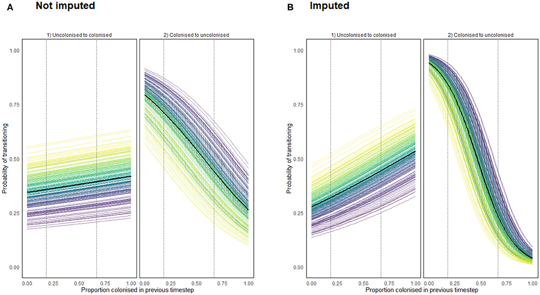
Figure 11. Transition probabilities from a state of uncolonization (by Campylobacter) to colonization, and from colonization to uncolonization using a density dependent model programmed using (A) recorded data (B) recorded and imputed data. Each colored line represents the transition probabilities for a single chicken, with a black line depicting the flock mean. Dotted lines show the region for which data was available for such a flock colonization proportion.

Importantly Figure 11 confirms that density dependence is apparent within the flock. This was an important result to capture to reinforce the findings of model 6. It confirms that birds are influenced by the colonization prevalence of the flock, suggesting that the more resilient birds truly are less likely to become colonized, as opposed to just never becoming exposed to particularly virulent STs. Of interest here is that the probability of clearing colonization (transitioning to uncolonized) is affected far more by flock prevalence proportion than the probability of becoming colonized.

Discussion

An improved understanding of the transmission dynamics of Campylobacter among and within poultry flocks in the commercial environment is essential for the design of effective intervention strategies to reduce levels of human disease. Here, these dynamics were evaluated within a flock of broiler-breeder chickens through a series of seven models, each constructed to investigate and answer a specific question. The analyses demonstrated the extent to which data can capture and describe multiple underlying dynamical behaviors, when queried with modeling approaches.

A number of the analyses were consistent with the existence of a “Campylobacter super-shedder” state within the flock, with other “resilient” birds that rarely or never transmit Campylobacter (Models 1, 5, 6, and 7). These resilient birds persisted even with high levels of colonization amongst the remainder of the flock (Model 7). The existence of super-shedders, is well-documented for Salmonella colonization in chickens (Gopinath et al., 2012; Menanteau et al., 2018) and a small number of studies indicate varied shedding levels of Campylobacter amongst cattle (Rapp et al., 2012); however, although the models presented here were developed from field data, there is otherwise a paucity of published evidence for a Campylobacter super-shedder status in chickens. This observation warrants further investigation, as the concept of individual colonization-resistant birds within a flock raises the potential of alternative approaches to controlling Campylobacter colonization in chicken flocks, e.g., those based on feed and/or probiotics. Small-scale experiments have shown that probiotic treatment can reduce Campylobacter bacterial load in individual birds (Willis and Reid, 2008; Ghareeb et al., 2012), but the wider impact in flock transmission dynamics is poorly understood. Numerical modeling approaches have, however, highlighted the growth rate of competing bacteria as the most powerful factor in reducing the spread of Campylobacter (Rawson et al., 2019).

The models further indicated that individual bird status was more important than Campylobacter strain in determining the dynamics of flock colonization (Models 6 and 7) and, to our knowledge, this is the first time this has been shown. Most (26/39, 66.7%) of the Campylobacter sequence types (STs) observed have been isolated from other chickens (Colles et al., 2015), which is consistent with them being competent at colonizing chicken hosts, although there is still potential for competition, for example over space or metabolic advantage. Whilst Campylobacter is generally considered to be a commensal of the chicken gut, there is evidence that in some breeds there is a prolonged inflammatory response, damage to the gut mucosa and diarrhea (Humphrey et al., 2014). Our results are consistent with the colonization of a chicken flock by Campylobacter being multi-factorial process, and the health and welfare of individual birds should be considered alongside Campylobacter strain type. The immune response of chickens has been shown to be impacted by welfare measures, such as stocking density (Guardia et al., 2011; Gomes et al., 2014), food withdrawal, and heat stress (Burkholder et al., 2008). Consequently these results suggest an additional incentive to uphold good bird welfare, as only a small sub-population of susceptible birds can have a large impact on the colonization status of the whole flock. The birds were weighed on two occasions through the study, but no correlation was found between weight and Campylobacter shedding rate.

Having confirmed the existence of variation in bird transition probabilities, the possible impact of such variation on the proliferation of Campylobacter STs was investigated. Using a previously-published stochastic differential equation model of Campylobacter population dynamics within a broiler flock (Rawson et al., 2019), two variant scenarios were explored: (i) one simulating a homogenous flock of chickens; and (ii) another simulating variation in immune response. The simulations demonstrated that demographically equal strains of Campylobacter could be sustained at broadly different levels across the flock as a consequence of bird immune response (Appendix 2). This is a random process, in that whichever strain is initially acquired by a super-shedder is then shed in large amounts into the environment, increasing the likelihood of colonizing other birds in the flock. This result implies that the observation that some STs persist at higher levels than others in the flock, is likely due to the variation in bird transition probabilities, as opposed to phenotypic differences between STs. For example, ST 958 may appear more than ST 45 (Figure 2), not because it has a competitive advantage, but because it was initially ingested by super-shedders. Indeed, upon examination of the first recorded appearance of specific STs, the STs that would appear most frequently throughout the experiment were first observed in the most susceptible birds. Likewise the STs that appeared to die out were first observed in the more resilient birds; however, as only 75 out of 200 birds were sampled each week the exact date of when a ST first occurred cannot be determined.

With respect to the two species, there was evidence that Campylobacter coli was shed by individual birds more consistently over time compared to Campylobacter jejuni, with some indication that C. coli was more prevalent in the winter and C. jejuni more prevalent in summer (Models 2, 3, and 4). These results should be interpreted with caution since, although the number of birds from which Campylobacter was detected was variable from week to week, single colony picks (i.e., one Campylobacter isolate per bird) were used, meaning the two variables were not entirely independent in this instance.

Human incidence of campylobacteriosis has been shown to vary in a repeated pattern each year (Nylen et al., 2002), which numerous studies have correlated with a similar pattern observed in broiler house colonization rates (Kapperud et al., 1993; Patrick et al., 2004; Jore et al., 2010), an observation disputed by other studies (Humphery et al., 1993). Despite this, there was no effect of seasonality on Campylobacter spp. shedding rate detected by the modeling approaches here (Models 1 and 3, Figures 4, 6), or in the original study examining local environmental variables (Colles et al., 2015). This lack of seasonality could be due to the different housing conditions and diet provisions between broiler and breeder flocks (Leeson and Summers, 2010). Breeder flocks have also been shown to shed smaller amounts of Campylobacter than commercial broilers (Cox et al., 2002).

The age of the flock has been shown to be an important factor associated with increasing Campylobacter strain diversity. C. coli are more commonly isolated from older broiler flocks and may be over-represented in this broiler-breeder flock in comparison to commercially housed broilers, who live for typically 5–10 weeks before slaughter. The finding, of increased colonization duration as time progressed (Model 3), primarily by C. coli, was most likely due to the increased flock prevalence resulting in a positive feedback loop, whereby more Campylobacter is being shed into the environment by colonized birds, and then further ingested by the other birds in the flock before they are able to clear colonization. Biologically, there is some indication that C. coli differs from C. jejuni based upon its genomic structuring, with the majority of farm animal related C. coli isolates grouping into the large ST-828 clonal complex, and C. jejuni isolates forming around 40 complexes. The shorter colonization periods by C. jejuni (Models 4 and 6, Figures 8, 10) potentially reflects a stronger immune response from the host leading to control or clearance of STs, although this did not preclude colonization by other C. jejuni (or C. coli) STs. Due to the inherent nature of sampling, it is not possible to know if strains were cleared altogether, or if multiple Campylobacter strains colonized birds simultaneously, although the modeling methods used in this study were chosen to take this uncertainty into account as far as possible. These results further highlight the importance of individual bird responses in determining flock-wide prevalence, and further ecological competition hierarchy modeling could be applied to the same data to assess the impact this phenomenon has on ST population stability across time. If structured hierarchical competition could be verified, this would support our contention that flock-wide defensive strategies should be conducted at an individual bird level.

We also stress the importance of our final model in not just investigating the weekly bacterial prevalence turnover, but how it further substantiates the importance of bird-to-bird transmission. Without this one could argue from our earlier results that more resilient birds were simply the ones who did not ingest a more invasive ST. Figure 11 shows the influence of flock colonization proportion on transition probabilities. Most notably we see that the transition from uncolonized to colonized is affected less by total colonization prevalence than the transition from colonized to uncolonized. This means that in a highly colonized flock, uncolonized birds still have a possibility to not become colonized, while those who are already colonized will be far less likely to then clear their colonization. This would likely be caused by the immune system of currently uncolonized birds being just as likely as previously to prevent an initial colonization, but currently colonized birds will be more likely to add to their current bacterial load by ingesting more Campylobacter and reduce their likelihood of recovery.

In conclusion, these analyses have highlighted the diversity of individual bird response to bacterial challenge, and how this range of responses can be a key driver of Campylobacter prevalence dynamics. It is now important to find an observable metric that correlates with the resilience of a bird to colonization. If it were possible to identify “super-shedder” birds on the farm, targeted interventions could be instituted to improve their health, or to better inform industry of how to raise broiler flocks with low rates of shedding within a flock. Such super-shedders will amplify the prevalence of Campylobacter within a flock, leading to rapid colonization. Now that we have highlighted the critical role that bird health plays, future work must elucidate how one may act to help prevent the emergence of super-shedders within the flock.

Data Availability Statement

The original contributions presented in the study are publicly available. This data can be found here: https://osf.io/m5yua/. Further inquiries can be directed to Thomas Rawson, thomas.rawson@zoo.ox.ac.uk.

Author Contributions

FC collected the data. TR, RP, MM, and MB conceived the study. TR and RP built the models and wrote all associated code. TR wrote the manuscript. MD, FC, and MB supervised the project. All authors reviewed the manuscript.

Funding

This work was supported through an Engineering and Physical Sciences Research Council (EPSRC) (https://epsrc.ukri.org/) Systems Biology studentship award (EP/G03706X/1) to TR. The funders had no role in study design, data collection and analysis, decision to publish, or preparation of the manuscript. This work was further supported by the Biotechnology and Biological Science Research Council as part of the Animal Health and Welfare ERA-net call (grant number BB/N023803/1), the United Kingdom Food Standards Agency (grant number FS101013); the Wellcome Trust (grant number 087622 to MM); and National Institute for Health Research Health Protection Research Unit (NIHR HPRU) in Gastrointestinal Infections at the University of Oxford in partnership with Public Health England (PHE). The views expressed are those of the author(s) and not necessarily those of the BBSRC, FSA, NHS, the NIHR, the Department of Health or Public Health England.

Conflict of Interest

The authors declare that the research was conducted in the absence of any commercial or financial relationships that could be construed as a potential conflict of interest.

Acknowledgments

This manuscript has been released as a pre-print at Rawson et al. (2020).

Supplementary Material

The Supplementary Material for this article can be found online at: https://www.frontiersin.org/articles/10.3389/fmicb.2020.576646/full#supplementary-material

References

Achen, M., Morishita, T. Y., and Ley, E. C. (1998). Shedding and colonization of Campylobacter jejuni in broilers from day-of-hatch to slaughter age. Avian Dis. 42, 732–737. doi: 10.2307/1592708

PubMed Abstract | CrossRef Full Text | Google Scholar

Aroori, S. V., Cogan, T. A., and Humphrey, T. J. (2013). The effect of growth temperature on the pathogenicity of Campylobacter. Curr. Microbiol. 67, 333–340. doi: 10.1007/s00284-013-0370-1

PubMed Abstract | CrossRef Full Text | Google Scholar

Barrow, P., Bumstead, N., Marston, K., Lovell, M., and Wigley, P. (2004). Faecal shedding and intestinal colonization of Salmonella enterica in in-bred chickens: the effect of host-genetic background. Epidemiol. Infect. 132, 117–126. doi: 10.1017/S0950268803001274

PubMed Abstract | CrossRef Full Text | Google Scholar

Bull, S., Allen, V., Domingue, G., Jørgensen, F., Frost, J., Ure, R., et al. (2006). Sources of Campylobacter spp. colonizing housed broiler flocks during rearing. Appl. Environ. Microbiol. 72, 645–652. doi: 10.1128/AEM.72.1.645-652.2006

PubMed Abstract | CrossRef Full Text | Google Scholar

Burkholder, K., Thompson, K., Einstein, M., Applegate, T., and Patterson, J. (2008). Influence of stressors on normal intestinal microbiota, intestinal morphology, and susceptibility to Salmonella enteritidis colonization in broilers. Poultry Sci. 87, 1734–1741. doi: 10.3382/ps.2008-00107

CrossRef Full Text | Google Scholar

Calderón-Gómez, L. I., Hartley, L. E., McCormack, A., Ringoir, D. D., and Korolik, V. (2009). Potential use of characterised hyper-colonising strain (s) of Campylobacter jejuni to reduce circulation of environmental strains in commercial poultry. Vet. Microbiol. 134, 353–361. doi: 10.1016/j.vetmic.2008.09.055

PubMed Abstract | CrossRef Full Text | Google Scholar

Colles, F. M., Jones, T. A., McCarthy, N. D., Sheppard, S. K., Cody, A. J., Dingle, K. E., et al. (2008). Campylobacter infection of broiler chickens in a free-range environment. Environ. Microbiol. 10, 2042–2050. doi: 10.1111/j.1462-2920.2008.01623.x

PubMed Abstract | CrossRef Full Text | Google Scholar

Colles, F. M., McCarthy, N. D., Bliss, C. M., Layton, R., and Maiden, M. C. (2015). The long-term dynamics of Campylobacter colonizing a free-range broiler breeder flock: an observational study. Environ. Microbiol. 17, 938–946. doi: 10.1111/1462-2920.12415

PubMed Abstract | CrossRef Full Text | Google Scholar

Cox, N., Stern, N., Musgrove, M., Bailey, J., Craven, S., Cray, P., et al. (2002). Prevalence and level of Campylobacter in commercial broiler breeders (parents) and broilers. J. Appl. Poultry Res. 11, 187–190. doi: 10.1093/japr/11.2.187

CrossRef Full Text | Google Scholar

De Cesare, A., Parisi, A., Bondioli, V., Normanno, G., and Manfreda, G. (2008). Genotypic and phenotypic diversity within three Campylobacter populations isolated from broiler ceca and carcasses. Poultry Sci. 87, 2152–2159. doi: 10.3382/ps.2007-00441

PubMed Abstract | CrossRef Full Text | Google Scholar

Dorazio, R. M. (2016). Bayesian data analysis in population ecology: motivations, methods, and benefits. Popul. Ecol. 58, 31–44. doi: 10.1007/s10144-015-0503-4

CrossRef Full Text | Google Scholar

EFSA Panel on Biological Hazards (2011). Scientific opinion on Campylobacter in broiler meat production: control options and performance objectives and/or targets at different stages of the food chain. EFSA J. 9:2105. doi: 10.2903/j.efsa.2011.2105

CrossRef Full Text | Google Scholar

Evans, S., and Sayers, A. (2000). A longitudinal study of Campylobacter infection of broiler flocks in great britain. Prev. Vet. Med. 46, 209–223. doi: 10.1016/S0167-5877(00)00143-4

PubMed Abstract | CrossRef Full Text | Google Scholar

Gelman, A. (2006). Prior distributions for variance parameters in hierarchical models (comment on article by Browne and Draper). Bayesian Anal. 1, 515–534. doi: 10.1214/06-BA117A

CrossRef Full Text | Google Scholar

Ghareeb, K., Awad, W., Mohnl, M., Porta, R., Biarnes, M., Böhm, J., et al. (2012). Evaluating the efficacy of an avian-specific probiotic to reduce the colonization of Campylobacter jejuni in broiler chickens. Poultry Sci. 91, 1825–1832. doi: 10.3382/ps.2012-02168

PubMed Abstract | CrossRef Full Text | Google Scholar

Gomes, A., Quinteiro-Filho, W. M., Ribeiro, A., Ferraz-de Paula, V., Pinheiro, M., Baskeville, E., et al. (2014). Overcrowding stress decreases macrophage activity and increases Salmonella enteritidis invasion in broiler chickens. Avian Pathol. 43, 82–90. doi: 10.1080/03079457.2013.874006

PubMed Abstract | CrossRef Full Text | Google Scholar

Gopinath, S., Carden, S., and Monack, D. (2012). Shedding light on Salmonella carriers. Trends Microbiol. 20, 320–327. doi: 10.1016/j.tim.2012.04.004

PubMed Abstract | CrossRef Full Text | Google Scholar

Grant, A. J., Coward, C., Jones, M. A., Woodall, C. A., Barrow, P. A., and Maskell, D. J. (2005). Signature-tagged transposon mutagenesis studies demonstrate the dynamic nature of cecal colonization of 2-week-old chickens by Campylobacter jejuni. Appl. Environ. Microbiol. 71, 8031–8041. doi: 10.1128/AEM.71.12.8031-8041.2005

PubMed Abstract | CrossRef Full Text | Google Scholar

Guardia, S., Konsak, B., Combes, S., Levenez, F., Cauquil, L., Guillot, J.-F., et al. (2011). Effects of stocking density on the growth performance and digestive microbiota of broiler chickens. Poultry Sci. 90, 1878–1889. doi: 10.3382/ps.2010-01311

PubMed Abstract | CrossRef Full Text | Google Scholar

Hermans, D., Van Deun, K., Messens, W., Martel, A., Van Immerseel, F., Haesebrouck, F., et al. (2011). Campylobacter control in poultry by current intervention measures ineffective: urgent need for intensified fundamental research. Vet. Microbiol. 152, 219–228. doi: 10.1016/j.vetmic.2011.03.010

PubMed Abstract | CrossRef Full Text | Google Scholar

Höök, H., Fattah, M. A., Ericsson, H., Vågsholm, I., and Danielsson-Tham, M.-L. (2005). Genotype dynamics of Campylobacter jejuni in a broiler flock. Vet. Microbiol. 106, 109–117. doi: 10.1016/j.vetmic.2004.12.017

PubMed Abstract | CrossRef Full Text | Google Scholar

Humphery, T., Henley, A., and Lanning, D. (1993). The colonization of broiler chickens with Campylobacter jejuni: some epidemiological investigations. Epidemiol. Infect. 110, 601–607. doi: 10.1017/S0950268800051025

CrossRef Full Text | Google Scholar

Humphrey, S., Chaloner, G., Kemmett, K., Davidson, N., Williams, N., Kipar, A., et al. (2014). Campylobacter jejuni is not merely a commensal in commercial broiler chickens and affects bird welfare. MBio 5:e01364-14. doi: 10.1128/mBio.01364-14

PubMed Abstract | CrossRef Full Text | Google Scholar

Jore, S., Viljugrein, H., Brun, E., Heier, B., Borck, B., Ethelberg, S., et al. (2010). Trends in Campylobacter incidence in broilers and humans in six European countries, 1997–2007. Prev. Vet. Med. 93, 33–41. doi: 10.1016/j.prevetmed.2009.09.015

PubMed Abstract | CrossRef Full Text | Google Scholar

Jorgensen, F., Ellis-Iversen, J., Rushton, S., Bull, S., Harris, S., Bryan, S., et al. (2011). Influence of season and geography on Campylobacter jejuni and C. coli subtypes in housed broiler flocks reared in great Britain. Appl. Environ. Microbiol. 77, 3741–3748. doi: 10.1128/AEM.02444-10

PubMed Abstract | CrossRef Full Text | Google Scholar

Jorgensen, F., Madden, R. H., Arnold, E., Charlett, A., and Elviss, N. C. (2015). FSA Project fs241044–Survey Report–A Microbiological Survey of Campylobacter Contamination in Fresh Whole UK Produced Chilled Chickens at Retail Sale (2014–15). London: Food Standards Agency.

Kapperud, G., Skjerve, E., Vik, L., Hauge, K., Lysaker, A., Aalmen, I., et al. (1993). Epidemiological investigation of risk factors for Campylobacter colonization in Norwegian broiler flocks. Epidemiol. Infect. 111, 245–256. doi: 10.1017/S0950268800056958

PubMed Abstract | CrossRef Full Text | Google Scholar

Kovats, R. S., Edwards, S. J., Charron, D., Cowden, J., D'Souza, R. M., Ebi, K. L., et al. (2005). Climate variability and Campylobacter infection: an international study. Int. J. Biometeorol. 49, 207–214. doi: 10.1007/s00484-004-0241-3

PubMed Abstract | CrossRef Full Text | Google Scholar

Kruschke, J. (2014). Doing Bayesian Data Analysis: A Tutorial With R, JAGS, and Stan. London; San Diego, CA; Waltham, MA; Oxford: Academic Press.

Kudirkienė, E., Malakauskas, M., Malakauskas, A., Bojesen, A. M., and Olsen, J. E. (2010). Demonstration of persistent strains of Campylobacter jejuni within broiler farms over a 1-year period in Lithuania. J. Appl. Microbiol. 108, 868–877. doi: 10.1111/j.1365-2672.2009.04490.x

PubMed Abstract | CrossRef Full Text | Google Scholar

Leeson, S., and Summers, J. D. (2010). Broiler Breeder Production. Nottingham: Nottingham University Press.

Menanteau, P., Kempf, F., Trotereau, J., Virlogeux-Payant, I., Gitton, E., Dalifard, J., et al. (2018). Role of systemic infection, cross contaminations and super-shedders in Salmonella carrier state in chicken. Environ. Microbiol. 20, 3246–3260. doi: 10.1111/1462-2920.14294

PubMed Abstract | CrossRef Full Text | Google Scholar

Nylen, G., Dunstan, F., Palmer, S., Andersson, Y., Bager, F., Cowden, J., et al. (2002). The seasonal distribution of Campylobacter infection in nine European countries and New Zealand. Epidemiol. Infect. 128, 383–390. doi: 10.1017/S0950268802006830

PubMed Abstract | CrossRef Full Text | Google Scholar

Patrick, M. E., Christiansen, L. E., Wainø, M., Ethelberg, S., Madsen, H., and Wegener, H. C. (2004). Effects of climate on incidence of Campylobacter spp. in humans and prevalence in broiler flocks in Denmark. Appl. Environ. Microbiol. 70, 7474–7480. doi: 10.1128/AEM.70.12.7474-7480.2004

PubMed Abstract | CrossRef Full Text | Google Scholar

Plummer, M. (2007). Jags: A Program for Analysis of Bayesian Graphical Models Using Gibbs Sampling. Available online at: http://mcmc-jags.sourceforge.net/

Google Scholar

Plummer, M., Stukalov, A., and Denwood, M. (2016). rjags: Bayesian Graphical Models Using MCMC. Available online at: https://cran.r-project.org/web/packages/rjags/index.html

Rapp, D., Ross, C. M., Pleydell, E. J., and Muirhead, R. W. (2012). Differences in the fecal concentrations and genetic diversities of Campylobacter jejuni populations among individual cows in two dairy herds. Appl. Environ. Microbiol. 78, 7564–7571. doi: 10.1128/AEM.01783-12

PubMed Abstract | CrossRef Full Text | Google Scholar

Rawson, T., Dawkins, M. S., and Bonsall, M. B. (2019). A mathematical model of Campylobacter dynamics within a broiler flock. Front. Microbiol. 10:1940. doi: 10.3389/fmicb.2019.01940

PubMed Abstract | CrossRef Full Text | Google Scholar

Rawson, T., Paton, R., Colles, F. M., Maiden, M. C., Dawkins, M. S., and Bonsall, M. B. (2020). A mathematical modelling approach to uncover factors influencing the spread of Campylobacter in a flock of chickens. bioRxiv. doi: 10.1101/2020.06.03.132191

CrossRef Full Text | Google Scholar

Shanker, S., Lee, A., and Sorrell, T. (1990). Horizontal transmission of Campylobacter jejuni amongst broiler chicks: experimental studies. Epidemiol. Infect. 104, 101–110. doi: 10.1017/S0950268800054571

PubMed Abstract | CrossRef Full Text | Google Scholar

Shreeve, J., Toszeghy, M., Pattison, M., and Newell, D. (2000). Sequential spread of Campylobacter infection in a multipen broiler house. Avian Dis. 44, 983–988. doi: 10.2307/1593076

PubMed Abstract | CrossRef Full Text | Google Scholar

Stern, N. J., Cox, N. A., Musgrove, M. T., and Park, C. (2001). Incidence and levels of Campylobacter in broilers after exposure to an inoculated seeder bird. J. Appl. Poultry Res. 10, 315–318. doi: 10.1093/japr/10.4.315

CrossRef Full Text | Google Scholar

Strachan, N. J., and Forbes, K. J. (2010). The growing UK epidemic of human campylobacteriosis. Lancet 376, 665–667. doi: 10.1016/S0140-6736(10)60708-8

PubMed Abstract | CrossRef Full Text | Google Scholar

Tam, C. C., and O'Brien, S. J. (2016). Economic cost of Campylobacter, norovirus and rotavirus disease in the United Kingdom. PLoS ONE 11:e0138526. doi: 10.1371/journal.pone.0138526

PubMed Abstract | CrossRef Full Text | Google Scholar

Tresse, O., Alvarez-Ordóñez, A., and Connerton, I. F. (2017). About the foodborne pathogen Campylobacter. Front. Microbiol. 8:1908. doi: 10.3389/fmicb.2017.01908

PubMed Abstract | CrossRef Full Text | Google Scholar

Wallace, J., Stanley, K., Currie, J., Diggle, P., and Jones, K. (1997). Seasonality of thermophilic Campylobacter populations in chickens. J. Appl. Microbiol. 82, 219–224. doi: 10.1111/j.1365-2672.1997.tb02854.x

PubMed Abstract | CrossRef Full Text | Google Scholar

Wigley, P. (2015). Blurred lines: pathogens, commensals, and the healthy gut. Front. Vet. Sci. 2:40. doi: 10.3389/fvets.2015.00040

PubMed Abstract | CrossRef Full Text | Google Scholar

Willis, W. L., and Reid, L. (2008). Investigating the effects of dietary probiotic feeding regimens on broiler chicken production and Campylobacter jejuni presence. Poultry Sci. 87, 606–611. doi: 10.3382/ps.2006-00458

PubMed Abstract | CrossRef Full Text | Google Scholar

Wilson, D. J., Gabriel, E., Leatherbarrow, A. J., Cheesbrough, J., Gee, S., Bolton, E., et al. (2008). Tracing the source of campylobacteriosis. PLoS Genet. 4:e1000203. doi: 10.1371/journal.pgen.1000203

PubMed Abstract | CrossRef Full Text | Google Scholar